應用於主動式攝影機上的權重式重取樣粒子濾波器的人形追蹤

國 立 交 通 大 學

多媒體工程研究所

碩 士 論 文

應用於主動式攝影機上的權重式重取樣粒子濾

波器的人形追蹤

Weighted resampling particle filter for human

tracking on an active camera

研 究 生：張良成

指導教授：林進燈 教授

i

應用於主動式攝影機上的權重式重取樣粒子濾波器的人形

追蹤

Weighted resampling particle filter for human tracking on an

active camera

研 究 生：張良成

Student：Liang-Cheng Chang

指導教授：林進燈 教授

Advisor：Prof. Chin-Teng Lin

國立交通大學

多媒體工程研究所

碩士論文

A Thesis

Submitted to Institute of Multimedia Engineering

College of Computer Science

National Chiao Tung University

in Partial Fulfillment of the Requirements

for the Degree of Master

in

Computer Science

July 2012

Hsinchu, Taiwan, Republic of China

ii

應用於主動式攝影機上的權重式重取樣粒子濾

波器的人形追蹤

學生：張良成

指導教授：林進燈 教授

國立交通大學 多媒體工程研究所碩士班

摘要

我們提出了權重式重取樣粒子濾波器演算法，並應用於主動式攝影機上做人 形追蹤。本系統主要有三部分，分別是人形偵測，人形追蹤和攝影機的控制。在 人形偵測方面使用編碼比對去得到人形區域，而粒子濾波器會對每張輸入的影片 估測出人形的位置。我們在重取樣中選擇具有高權重的粒子，因為這能讓追蹤特 徵更精確。此外比例-積分-微分控制器(PID controller)用來控制主動式攝影機，藉 由最小化介於影片中心和物體位置的誤差，並轉換此誤差為 pan-tilt 速度來驅動 攝影機移動讓被追蹤的人保持在影片的可視範圍內。在追蹤過程中，影像的強度 和人的特徵也會隨之變化。因此高斯混和模型(GMM)會隨著時間來更新人的特 徵模型。至於短暫的遮蔽問題可透過特徵相似度和重新取樣粒子來解決。而粒子 濾波器能估測出每張輸入影像裡人形的位置，因此可以平滑地驅動主動式攝影 機。

iii

Weighted resampling particle filter for human

tracking on an active camera

Student: Liang-Cheng Chang

Advisor: Prof. Chin-Teng Lin

Institute of Multimedia Engineering

National Chiao Tung University

Abstract

We proposed a weighted resampling algorithm for particle filter and applied for human tracking on active camera. The system consists of three major parts which are human detection, human tracking, and camera control. The codebook matching algorithm is used to extract human region in human detection system, and the particle filter algorithm is estimating the position of the human in every input image. We select particles with high weighting value in resampling, because it will give higher accurate tracking features. Moreover, a proportional–integral–derivative controller (PID controller) controls the active camera by minimizing difference between center of image and the object’s position obtained from particle filter, also convert the position difference into pan-tilt speed to drive the active camera and keep the human in the field of view (FOV) camera. The intensity of image may change over tracking, and so do the human features. Therefore, the Gaussian mixture model (GMM) algorithm is used to update the human feature model overtime. As regards, the temporal occlusion problem is solved by feature similarity and the resampling particles. Also, the particle filter is estimating the position of human in every input frames, thus the active camera will drive smoothly.

iv

致謝

兩年的碩士班生活即將劃下句點，能得到各位老師的指點是我此生的榮幸， 尤其是指導教授林進燈博士這兩年來的細心教導，讓我學習到許多寶貴的知識與 經驗，在學業及研究方法上也受益良多。另外也要感謝口試委員陶金旺博士、張 志永博士與陳永平博士在口試時的指點與鼓勵，使得本論文更為完整。 其次感謝超視覺實驗室的 Linda、子貴、建霆、肇廷、東霖、勝智、Mukesh、 洸本所有學長姐給予我指導與建議，尤其是 Linda 學姊給予我許多建議與方向， 讓我能順利完成論文。也感謝同學廷維、庭伊、榮宗的相互砥礪，還有實驗室的 學弟宗濬、柏羲、峪鋒、建維、威良，在生活上給予諸多的協助，讓我在這兩年 的研究生涯，無論是課業上、學業上或是生活上都不孤單。 最後，更要感謝我的父母，從小到大的教育及栽培，在研究所這段時間裡讓 我無後顧之憂，如果沒有他們無怨無悔的付出，就沒有今日的我。 謹以本論文獻給我的家人及所有關心我的師長與朋友們。

v

Contents

致謝... iv

Contents ... v

List of Tables ... vii

List of Figures ... viii

Chapter 1 Introduction ... 1

1.1 Motivation ... 2

1.2 Objective ... 2

1.3 Related work ... 3

1.4 System architecture ... 7

Chapter 2 Human detection ... 9

2.1 Moving object extraction ... 9

2.2 Codebook matching ... 11

Chapter 3 Human tracking ... 13

3.1 Histogram color features ... 13

3.2 Kernel function ... 15

3.3 Particle filter algorithm ... 17

3.4 Weighted resampling algorithm ... 20

3.5 Target update ... 21

3.6 Occlusion handler ... 23

Chapter 4 Camera control ... 25

4.1 PID controller... 27

4.2 Zoom in/out control ... 30

Chapter 5 Experimental results ... 31

5.1 Track on video file ... 31

vi

Chapter 6 Conclusions and Future work ... 42

6.1 Conclusions ... 42

6.2 Future works ... 43

vii

List of Tables

Table 5-1 Zoom layer varies in Fig. 5-6 ... 38 Table 5-2 Zoom layer varies in Fig. 5-7 ... 39

viii

List of Figures

Fig. 1-1 Three categories of tracking ... 4

Fig. 1-2 System overview ... 7

Fig. 2-1 Human detection system ... 9

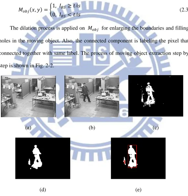
Fig. 2-2 The results in moving object extraction. (a)𝑰_𝑩 (b)𝑰_𝑪 (c)𝑴_𝒐𝒃𝒋 (d)𝑰_𝑫 (e)𝑰_𝑹𝑶𝑰 ... 10

Fig. 2-3 Codebook matching... 11

Fig. 2-4 Feature word X ... 11

Fig. 2-5 The procedure of the comparison with the codebook ... 12

Fig. 3-1 (a) RGB color model (b) HSV color model ... 14

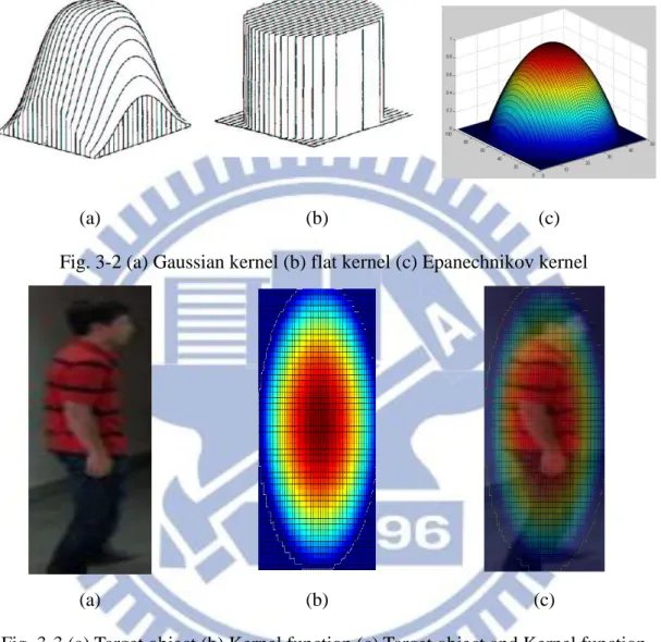
Fig. 3-2 (a) Gaussian kernel (b) flat kernel (c) Epanechnikov kernel ... 16

Fig. 3-3 (a) Target object (b) Kernel function (c) Target object and Kernel function .. 16

Fig. 3-4 Weighted resampling particle filter ... 20

Fig. 3-5 Original resampling ... 20

Fig. 3-6 Weighted resample ... 21

Fig. 3-7 Occlusion handler (a) frame 681 (b) frame 685 (c) frame 690 (d) frame 69524 Fig. 3-8 Occlusion handler flow chart ... 24

Fig. 4-1 Active camera control through RS485 ... 25

Fig. 4-2 Message format ... 25

Fig. 4-3 Data byte 1 to 4 format ... 26

Fig. 4-4 Control direction for each regions ... 26

Fig. 4-5 Camera control flow chart ... 27

Fig. 4-6 The PID controller ... 28

Fig. 5-1 Tracking without occlusion handler ... 32

Fig. 5-2 Tracking with occlusion handler ... 33

Fig. 5-3 Object has similar color as target human ... 34

Fig. 5-4 (a) frame 1436, 1547 and 1605 (b) frame 2152, 2214 and 2277 ... 35

Fig. 5-5 Update pan and tilt command to track ... 37

Fig. 5-6 The effects of zoom in / out ... 38

Fig. 5-7 Combination of pan, tilt and zoom in / out ... 39

Fig. 5-8 Human tracking in multiple objects ... 40

1

1

Chapter 1

Introduction

In recent years, visual-based detection and tracking methods have been applied to security surveillance to improve safety and convenience of human’s life. Traditional visual-based surveillance system uses human eyes to check monitor all day. This is inefficient and time consuming. In order to solve this problem, automatic and real-time vision based surveillance system has been proposed in this work.

In surveillance system, human detection and tracking are important topics. The human detection system has two parts: moving object extraction and human recognition. The moving object extraction extracts object from background and find its related position and size in an image. Human recognition recognizes object as human or nonhuman. Then, the tracking system will track the human in continuous frame. The human may be occluded with other objects while tracking. So the tracking system must able to predict the position during and after occlusion.

There are two kinds of camera used in surveillance system, which are fixed and active camera. The advantage of a fixed camera is low cost, but its FOV (field of view) is limited. On the other hand, active camera has good FOV because it has the ability to perform pan-tilt to keep target human in the camera scene. Also, it has good resolution because able to do zoom in/out.

In this thesis, we integrate human detection, human tracking, and active camera controller to achieve automatic and real-time surveillance systems.

2

1.1 Motivation

Commonly, tracking system on active camera uses temporal difference to extract moving object. In this process, we need to wait the camera stable enough to do image processing. In other word, the moving camera will capture blur images and extract not only moving object but also background pixels. Consequently, the active camera is driven discontinuously and non-smoothly. Therefore, we applies particle filter tracking algorithm to solve this problem. The codebook method is applied first to detect human as target model, then the particle filter tracks it by calculating the Bhattacharyya distance between target model’s color histogram with next frame color histogram of the sampled particle position. The color histogram has many advantages, for example it can track non-rigid object, robust to partial occlusion, rotation and scale invariant, also calculated efficiently.

1.2 Objective

The objective of this thesis is to construct a real-time human tracking system on active camera which has some characteristics as listed below.

1) It can detect human fast.

2) It can track without using background information. 3) It can handle occlusion condition.

4) It can drive active camera smoothly and continuously. 5) It can zoom in/out appropriately.

3

1.3 Related work

In this thesis, we classify the related work into three parts as follows, 1. Human detection

A human detection system determines the human’s position and its size in an image. Optical flow [1, 2] is used to estimating independently moving object, but it costs complex computation and sensitive to the change of intensity. Zhao et al [3] exploit stereo based segmentation algorithm to extract object from background, and recognizing the object by neural network. Although stereo vision based technique has been proved more robust, but it requires at least two cameras and cannot be used in long distance detection. Dalal and Triggs [4] computed oriented gradient and select the dominant orientated gradients to detect human. Sebastian and Alvaro [5] present a new computer vision algorithm which designed to operate with moving cameras and detect human in different poses under partial or complete view of the human body. Viola et al [6] proposed cascade Boosting detector, the AdaBoost iteratively constructs a strong classifier guided by user-specified performance criteria. The cascade approach is quickly rejecting non-pedestrian sample in early cascade layer, thus this method has high processing speed. A template-based approach [7] is presented to detect human silhouettes in a specific walking pose, and templates consist of short sequences of 2D silhouettes obtained from motion capture data. In order to detect human fast, we choose the shape-based human model to classify human being by codebook matching, which decreases the time of human detection from the other objects.

4

Fig. 1-1 Three categories of tracking 2. Human tracking

Human tracking is used to following target human through the sequence images in terms of changes in scale and position. Fig. 1-1 shows three based tracking method. First, feature based is the most commonly method, and color, edge, or motion is used as tracking feature. The edge detection method, such as Sobel method [8], Laplacian method [8], and Marr–Hildreth method [9], etc., utilize masks to do convolution on the image to detect the edges. Wei Guo et al. [10] propose human tracking system based on shape analysis. Law et al. [11] design fuzzy rules used in edge based human tracking. This method requires a rather large and complicated rules set, also need more computation time, and edge pixels cannot be always detected continuously. We noted that all those methods mentioned above detect edges using gray level images, and those methods will be neglect for color images because the representation of a pixel is not only a gray level but a vector in a color space. The edge occurring in the adjacent pixels which have the same values may not be detected. So, edge detection only in gray level image is not sufficient and robust.

Pattern recognition do learning the target object and search them in sequence image. Williams et al. [12] extended the approach to the nonlinear translation predictors which learned by Relevance Vector Machine. Agarwal and Triggs [13] used RVM to learn the linear and nonlinear mapping for tracking of 3D human poses from

5

silhouettes. Bohyung Han and Larry Davis [14] used PCA to extract feature from color and used these feature in mean-shift tracking algorithm. Robert T. et al. [15] presents an online feature selection mechanism for evaluating multiple features while tracking and adjusting the set of features to improving tracking performance. The feature evaluation mechanism is embedded in a mean-shift tracking system. It can adaptively select features for tracking. The mean-shift algorithm was originally proposed by Fukunaga and Hostetler [16] for clustering data. The kernel-based object tracking is proposed by Meer et al [17]. This method tracks an object region represented by a spatial weighted intensity histogram, and computed its similarity value by Bhattacharyya distance using iterative mean-shift algorithm. Later, many variants of the mean-shift algorithm were proposed for various applications [18-21]. Although the mean-shift object tracking algorithm performs well on sequences with relatively small object displacement, however its performance is not guaranteed when objects undergo partial or full occlusion. In order to improve the performance of mean-shift tracker under partial occlusion, there some algorithms added to the mean-shift such as Kalman filter [22-23] or particle filter [24-25]. K. Nummiaro et al [25] use the idea of particle filter to apply a recursive Bayesian filter based on sample sets. They use color as feature. Their work has evolved from the condensation algorithm which was developed in the computer vision community. In this thesis, we select the particle filter to track human, because it has proven very successful for non-linear and non-Gaussian estimation problems.

3. Camera

Tracking object with an active camera can drive pan-tilt to keep the object in the scene of camera and use zoom in/out to adjust the resolution of object. Many tracking system work only on pan/tilt or zoom. Murray et al. [26] utilized morphological filtering of motion images for background compensation. It can track a moving object

6

from dynamic images with drive pan-tilt angles. C. Lin et al. [27] use an image mosaic technique to track moving objects with a single pan-tilt camera for indoors environment. Collins et al. [28] developed a system with multiple cameras that tracked a moving figure using pan-tilt cameras alone. This system used a kernel-based tracking approach to overcome the apparent motion of the background while the camera moved. L. Fiore et al. [29] used wide angle and active camera to achieve human tracking. In this work the target object was found by wide angle camera and through camera calibration method tell the active camera to drive pan-tilt to track to the specific object position. The objective of our approach is driving pan-tilt to keep target in the center of FOV. If the target’s size is smaller or larger than a minimum or maximum size, then the zoom function will drive zoom-in or zoom-out. In order to drive active camera smoothly and continuously, we use PID controller, because it can minimize the error between target and center of camera’s FOV. Also, we use the target ROI size which estimated by particle filter to determine zoom-in or zoom-out.

7

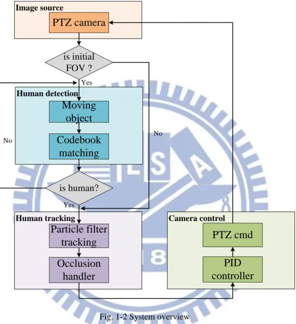
1.4 System architecture

Yes No Human detection

Moving

object

Codebook

matching

Yes No Image source

PTZ camera

Human tracking

Particle filter

tracking

Occlusion

handler

Camera control

PID

controller

PTZ cmd

is initial FOV ? is human?

Fig. 1-2 System overview

The whole system consists four major parts: Image source, Human detection, Human tracking, and Camera control. The input frames are captured by PTZ camera with resolution 720*480. The initial FOV is the scene we want to monitor. Moving object will be extracted by background difference. The codebook matching is applied to classify the moving object into human or nonhuman. When a human is detected in initial FOV, we regard it as target. The Particle filter algorithm will track the target in every frame also send the target position and size to camera control. The occlusion

8

handler uses the similarity value in every frame to solve the temporal full occlusion that sometimes leads to tracking lost in particle filter. The Target position is sent to PID controller to determine pan-tilt speed and the size is used to decide zoom-in or zoom-out. The PTZ cmd will drive PTZ to keep the target in the center of FOV. When PTZ camera is driven, it changes FOV. And the human detection is skipped during camera tracking.

9

2

Chapter 2

Human detection

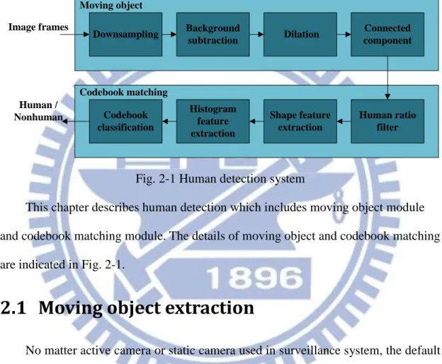
Downsampling Background subtraction Dilation Connected component Shape feature extraction Human ratio filter Histogram feature extraction Codebook classification Moving object Codebook matching Image frames Human / Nonhuman

Fig. 2-1 Human detection system

This chapter describes human detection which includes moving object module and codebook matching module. The details of moving object and codebook matching are indicated in Fig. 2-1.

2.1 Moving object extraction

No matter active camera or static camera used in surveillance system, the default position of camera is mostly fixed. So, we can use background subtraction to extract moving object. The background subtraction only uses gray level image, so it can decrease the computing power and achieve real-time requirement. The background image is constructed by using the first frame, and adapted as time using Eq. 2.1.

𝐼_𝐵𝑛_{(𝑥, 𝑦) = {}𝛼 ∗ 𝐼𝐵𝑛−1(𝑥, 𝑦) + (1 − 𝛼) ∗ 𝐼𝑐(𝑥, 𝑦), 𝐼𝑀(𝑥, 𝑦) = 0

𝐼_𝐵𝑛−1_{(𝑥, 𝑦), 𝐼}

𝑀(𝑥, 𝑦) = 1 (2.1)

where 𝐼_𝐵𝑛 and 𝐼_𝐵𝑛−1 represent current and previous background image, respectively.

10

active pixel between previous frame and current frame.

The moving object 𝐼_𝐵𝑆 is calculated from difference between current image 𝐼_𝑐 and background image 𝐼_𝐵 as written below.

𝐼_𝐵𝑆(𝑥, 𝑦) = |𝐼_𝑐(𝑥, 𝑦) − 𝐼_𝐵(𝑥, 𝑦)| (2.2) A threshold value ths is determined for producing binary moving object 𝑀_𝑜𝑏𝑗 as described in Eq. 2.3.

𝑀𝑜𝑏𝑗(𝑥, 𝑦) = {1, 𝐼𝐵𝑆 ≥ 𝑡ℎ𝑠

0, 𝐼𝐵𝑆 < 𝑡ℎ𝑠

(2.3) The dilation process is applied on 𝑀𝑜𝑏𝑗 for enlarging the boundaries and filling

holes in the moving object. Also, the connected component is labeling the pixel that connected together with same label. The process of moving object extraction step by step is shown in Fig. 2-2.

(a) (b) (c)

(d) (e)

11

2.2 Codebook matching

Moving objet Normalize Shape feature

extraction Histogram feature extraction Feature matching with codebook Human / Nonhuman

Fig. 2-3 Codebook matching

The codebook matching algorithm in this thesis is based on human-shape information. At first, the moving object obtained from moving object extraction is normalized into (20*40). The shape feature extraction extracts the position of shape pixels in an image, as pointed by red dot in Fig. 2-4. Ten Y-axis coordinates are chosen for leftmost and rightmost of object’s boundary. Then, the twenty coordinates of its related X-axis coordinate are arranged as feature vector as shown as blue blocks in Fig. 2-4.

The projection of X-axis calculates the histogram of pixel values on the Y-axis. Total bin of the histogram is ten as shown as green blocks in Fig. 2-4. Therefore, an object can be representing as 30-feature vector in our work.

12

By observation, the top and bottom of Y-axis of shape pixels are not suitable to choose as feature points, because these pixels are changeable. The way to find ten specific coordinates at Y-axis is to calculate the standard deviation in each value of Y-axis for a training sample, and then chooses ten lowest standard deviation values each side.

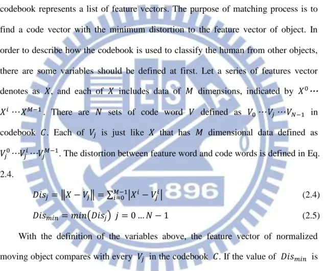
The feature vector is matched with the code vectors in the codebook. The codebook represents a list of feature vectors. The purpose of matching process is to find a code vector with the minimum distortion to the feature vector of object. In order to describe how the codebook is used to classify the human from other objects, there are some variables should be defined at first. Let a series of features vector denotes as 𝑋, and each of 𝑋 includes data of 𝑀 dimensions, indicated by 𝑋0… 𝑋𝑖_…𝑋𝑀−1_{. There are 𝑁 sets of code word 𝑉 defined as 𝑉}

0…𝑉𝑗…𝑉𝑁−1 in

codebook 𝐶. Each of 𝑉𝑗 is just like 𝑋 that has 𝑀 dimensional data defined as

𝑉_𝑗0…𝑉_𝑗𝑖…𝑉_𝑗𝑀−1_{. The distortion between feature word and code words is defined in Eq.}

2.4.

𝐷𝑖𝑠𝑗 = ‖𝑋 − 𝑉𝑗‖ = ∑𝑀−1𝑖=0 |𝑋𝑖− 𝑉𝑗𝑖| (2.4)

𝐷𝑖𝑠_𝑚𝑖𝑛= 𝑚𝑖𝑛(𝐷𝑖𝑠_𝑗) 𝑗 = 0 … 𝑁 − 1 (2.5) With the definition of the variables above, the feature vector of normalized moving object compares with every 𝑉𝑗 in the codebook 𝐶. If the value of 𝐷𝑖𝑠𝑚𝑖𝑛 is

smaller than the threshold defined by user, the moving object with the feature word 𝑋 is considered as human. Otherwise, it is a nonhuman object. The demonstration of comparing 𝑋 with 𝑉_𝑗 is showed in Fig. 2-5.

13

3

Chapter 3

Human tracking

A human tracking system based on particle filter algorithm is proposed in this thesis. The key idea of particle filter is to approximate the probability distribution by a weighted sample set and each sample represents one hypothetical state of the object with a corresponding discrete sampling probability [25]. The original resample method selects sample using uniformly distributed random number. It usually keeps some low weighted samples which may decrease the accuracy of tracking. In this thesis, we proposed a weighted resampling particles method which just selects high weighted samples.

3.1 Histogram color features

Mostly, feature based object tracking method uses color as feature. Color information is more accurate than gray scale. Based on experiment, the HSV color space gives a good performance while tracking, thus we apply it on our tracking algorithm.

The main purpose of HSV color space is to reduce the sensitivity of illumination or lightness information of RGB color space. Fig. 3-1 (a), (b) shows RGB and HSV color space, respectively. The HSV model, also known as HSB model, was created in 1978 by Alvy Ray Smith. It is a nonlinear transformation of the RGB color space. It defines a color space in terms of three components: hue, saturation, and value. The definition is described below: [31]

14

1. Hue: It is the color type and ranges from 0 ~ 360 degree. Each value corresponds to one color. For example, 0 is red, 45 is orange and 55 yellow. When it comes to 360 degree, it is also equal to 0 degree.

2. Saturation: It is the intensity of the color, and ranges from 0%~100%. 0 means no color, and that means only gray value between black and white exists. 100 means the intense color with the most color variety.

3. Value: It is the brightness of the color, and also ranges from 0%~100%. 0 is always black. Depending on the saturation, 100 may be white or a more or less saturated color.

(a) (b)

Fig. 3-1 (a) RGB color model [31] (b) HSV color model [32]

The transformation from RGB color model to HSV color model is written in the following equation. 0 6 0 0 , 6 0 3 6 0 , 6 0 1 2 0 6 0 2 4 0 i f M A X M I N G B i f M A X R G B M A X M I N G B i f M A X R G B H _{M A X M I N} B R i f M A X G M A X M I N R G i f M A X B M A X M I N             _          _        _       (3.1)

15 0 0 1 i f M A X S _{M I N} O t h e r w i s e M A X        (3.2) V  M A X (3.3)

where MAX, MIN denote maximum and minimum value of (R, G, B), respectively. Generally, each color-channel has 8-bits data, means produce (256*256*256) of bins of color histogram. Without loss of generality, the color-data is quantizing into (6*6*6). Therefore, total bin of the color histogram is 216 bins.

3.2 Kernel function

Kernel function is used to represent a target object. Different statistical distributions can be adopted for both target object or candidate model, such as Gaussian kernel, Flat kernel and Epanechnikov kernel. Let x be normalized pixel as location in the region defined as target model, then the Gaussian kernel, Flat kernel and Epanechnikov kernel [33] are defined as follows.

1. Gaussian kernel 2 1 1 ( ) e x p ( || ||) 2 2 k x x    (3.4) 2. Flat kernel 1 || || 1 ( ) 0 if x k x o th e r w is e      (3.5) 3. Epanechnikov kernel 2 3 (1 ) || || 1 ( ) 4 0 x i f x k x o t h e r w i s e        (3.6) Fig. 3-2 (a) and (c) show the distribution of Gaussian and Epanechnikov kernel are similar. They have highest value are the center distribution. If we take a look at the ROI of target model in Fig. 3-3 (a), the pixels which are closer to the center of ROI is

16

containing more important information and the background pixels are mostly near at ROI’s boundary. Therefore, Gaussian and Epanechnikov kernel can disregard the boundary information and the accuracy will larger than flat kernel.

(a) (b) (c)

Fig. 3-2 (a) Gaussian kernel (b) flat kernel (c) Epanechnikov kernel

(a) (b) (c)

17

3.3 Particle filter algorithm

Particle filter provides a robust tracking framework, as it models uncertainty. It can keep its options open and consider multiple state hypotheses simultaneously. Since less likely object states have a chance to temporarily remain in the tracking process, particle filters can deal with short-lived occlusions [25].

Define target model at location-y as m-bin histogram 𝑞_𝑦 = {𝑞_𝑦(𝑢)}_{𝑢=1…𝑚} which compute by equation below.

𝑞_𝑦(𝑢) = 𝑓 ∑ 𝑘 (‖𝑦−𝑥𝑖‖

𝑎 ) 𝛿[ℎ(𝑥𝑖) − 𝑢] 𝐼

𝑖=1 (3.7)

with the normalized factor 𝑓 = 1

∑𝐼_𝑖=1𝑘(‖𝑦−𝑥𝑖‖_𝑎 ) (3.8)

where I denotes the number of pixels in the ROI region, 𝛿 is the Kronecker delta function, and a=√𝑤2_{+ ℎ}2 _{is used to normalize the size of the object region. The}

sample model 𝑝_𝑦 = {𝑝_𝑦(𝑢)}_{𝑢=1…𝑚} is represented as the same model as target model. The similarity value 𝜌 between target and sample model computes by Bhattacharyya distance d. Large 𝜌 means two models more similar, 𝜌 equal to 1 when two histograms are identical.

𝑝_𝑦(𝑢) = 𝑓 ∑ 𝑘 (‖𝑦−𝑥𝑖‖ 𝑎 ) 𝛿[ℎ(𝑥𝑖) − 𝑢] 𝐼 𝑖=1 (3.9) 𝜌[𝑝, 𝑞] = ∑𝑚 √𝑝(𝑢)_𝑞(𝑢) 𝑢=1 (3.10) 𝑑 = √1 − 𝜌[𝑝, 𝑞] (3.11)

In particle filter algorithm, the target model can be represented by a state vector 𝑠𝑡𝑎𝑟𝑔𝑒𝑡.

𝑠_{𝑡𝑎𝑟𝑔𝑒𝑡} = {x, 𝑣_𝑥, y, 𝑣_𝑦, w, h} (3.12)

18

denote the width and height of ROI, respectively.

The initial sample set 𝑆𝑖𝑛𝑖𝑡𝑖𝑎𝑙 = {𝑠(𝑛)}𝑛=1…𝑁 compute by

𝑠(𝑛) _{= 𝐼𝑠}

𝑡𝑎𝑟𝑔𝑒𝑡+ 𝑟. 𝑣. (3.13)

with 𝑁 is the number of samples, 𝐼 is an identity matrix, and 𝑟. 𝑣. is a multivariate Gaussian random variable.

The sample set is propagated through a dynamic model as following equation. 𝑠𝑡= 𝐴𝑠𝑡−1+ 𝑟. 𝑣.𝑡−1 (3.14)

where 𝐴 defines the deterministic component of the model. By using every sample’s weight and its state vector, the target human’s position and size can be obtained from estimated vector using following equation.

𝐸[𝑆_𝑡] = ∑𝑁 𝜔_𝑡(𝑛)

𝑛=1 𝑠𝑡(𝑛) (3.15)

The Bhattacharyya distance uses to update each sample’s weight as following equation. 𝜔(𝑛)₌ 1 √2𝜋𝜎𝑒 −_2𝜎2𝑑2 ₌ 1 √2𝜋𝜎𝑒 −(1−𝜌[𝑝_2𝜎2𝑠(𝑛),𝑞]) (3.16) The resample step avoids the problem of degeneracy of the algorithm, in other words, avoiding the situation that most sample weights are close to zero. The opportune moment of resample step is determined by following equation.

𝑁𝑒𝑓𝑓 < 𝑁𝑡ℎ𝑠 (3.17) 𝑁_𝑒𝑓𝑓 = 1 ∑𝑁 (𝜔_𝑡(𝑛))2 𝑛=1 (3.18) 𝑁_𝑡ℎ𝑠= 𝑟𝑎𝑡𝑒 ∗ 𝑁 (3.19)

where 𝑟𝑎𝑡𝑒 ∈ (0,1), 𝑁𝑒𝑓𝑓 and 𝑁𝑡ℎ𝑠 are the effective number of samples and given

of threshold sample, respectively. During resample step, samples with high weight may be chosen several times, leading to identical copies, while others with relatively low weights may not be chosen at all.

19

set to 𝑆_{𝑖𝑛𝑖𝑡𝑖𝑎𝑙}. The details particle filter algorithm for each iteration described as follow.

1. Propagate each sample from the set 𝑆𝑡−1 by a linear stochastic differential

equation:

𝑠_𝑡(𝑛) = 𝐴𝑠_𝑡−1(𝑛) + 𝑟. 𝑣._𝑡−1(𝑛)

2. Observe the color distributions:

(a) calculate the color distribution 𝑝

𝑠_𝑡(𝑛)

(𝑢) _{= 𝑓 ∑ 𝑘 (}‖𝑠𝑡(𝑛)−𝑥𝑖‖

𝑎 ) 𝛿[ℎ(𝑥𝑖) − 𝑢] 𝐼

𝑖=1 for each sample in the set 𝑆𝑡

(b) calculate the Bhattacharyya coefficient for each sample of the set 𝑆_𝑡 ρ [𝑝_𝑠

𝑡(𝑛), q] = ∑ √𝑝𝑠_𝑡(𝑛)

(𝑢)_𝑞(𝑢) 𝑚

𝑢=1

(c) weight each sample of the set 𝑆_𝑡 𝜔_𝑡(𝑛)= 1

√2𝜋𝜎𝑒

−(1−𝜌[𝑝𝑠𝑡(𝑛),𝑞])_2𝜎2

3. Estimate the mean state of the set 𝑆_𝑡

𝐸[𝑆_𝑡] = ∑𝑁 𝜔_𝑡(𝑛)

𝑛=1 𝑠𝑡(𝑛)

4. Resample the sample set 𝑆_𝑡, if 𝑁_𝑒𝑓𝑓 < 𝑁_𝑡ℎ𝑠

Select 𝑁 samples from the set 𝑆_𝑡 with probability 𝜔_𝑡(𝑛): (a) calculate the normalized cumulative probabilities 𝑐_𝑡′

𝑐_𝑡(0) = 0 𝑐_𝑡(𝑛) = 𝑐_𝑡(𝑛−1)+ 𝜔_𝑡(𝑛) 𝑐′ 𝑡 (𝑛) ₌ 𝑐_𝑡(𝑛) 𝑐_𝑡(𝑁)

(b) generate a uniformly distributed random number 𝑟 ∈ [0,1] (c) use binary search to find the smallest 𝑗 for which 𝑐′_𝑡(𝑗)≥ 𝑟 (d) set 𝑠′_𝑡(𝑛) = 𝑠_𝑡(𝑗)

20

Create target model & sample

set

Propagate

sample Observe sample

Estimate target state Weighted

resampling Target model has

been created Target is occlued End Yes No Yes No Target human

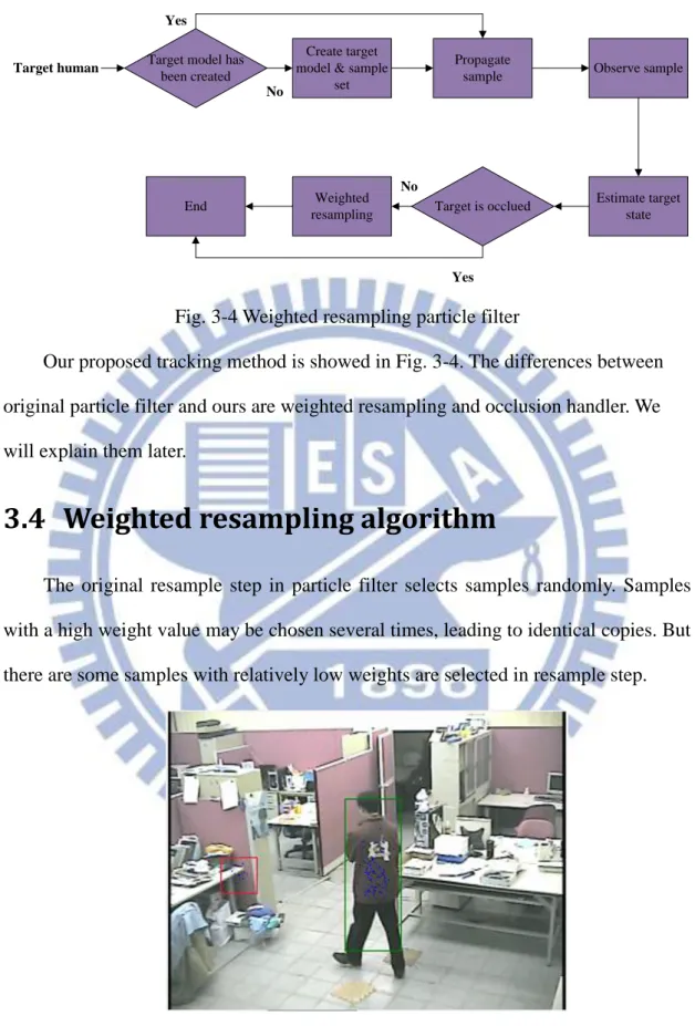
Fig. 3-4 Weighted resampling particle filter

Our proposed tracking method is showed in Fig. 3-4. The differences between original particle filter and ours are weighted resampling and occlusion handler. We will explain them later.

3.4 Weighted resampling algorithm

The original resample step in particle filter selects samples randomly. Samples with a high weight value may be chosen several times, leading to identical copies. But there are some samples with relatively low weights are selected in resample step.

Fig. 3-5 Original resampling

Fig.3-5 shows the samples points with high weights are in the ROI (green block), and samples with relatively low weights are in the red block. Although, two blocks

21

have nearly same similarity value, but the actual target object is in the green block. Consequently, it may track a different object as target object. In other word, it will decrease the accuracy of tracking. Thus, we proposed a weighted resampling algorithm to cover this problem. First, choose top sample set 𝑆_𝑡𝑡𝑜𝑝 with 𝑁_𝑡𝑜𝑝 weights from set 𝑆_𝑡.

𝑁_𝑡𝑜𝑝 = 𝑡𝑜𝑝 ∗ 𝑁 (3.20)

𝑆_𝑡𝑡𝑜𝑝 = {𝑠𝑡𝑜𝑝(𝑛)_}

𝑛=1…𝑁𝑡𝑜𝑝 (3.21)

where 𝑡𝑜𝑝 is a top rate which set to 0.2. The 𝑆_𝑡𝑡𝑜𝑝 just selecting samples with top 20% weights from set 𝑆_𝑡. Reproduce 𝑁 samples in 𝑆_𝑡 according to the weight of 𝑠𝑡𝑜𝑝(𝑛)_{. This step will produce 𝑠}𝑡𝑜𝑝(𝑛) _{which has relative high more times in 𝑆}

𝑡, and

others with relative low weight will be produced at least one time. Fig. 3-6 shows the weighted resampling result. Most of sample points lie in the green block or in the target object region.

Fig. 3-6 Weighted resample

3.5 Target update

The GMM (Gaussian Mixture Model) applies to update the target model over time. Let 𝐾 Gaussian distributions are chosen to approximate any continuous

22 probability distribution. 𝑝(𝑥) = ∑ 𝑝(𝑘)𝑝(𝑥|𝑘) = ∑𝐾 𝜋_𝑘𝑁(𝑥|𝜇_𝑘, 𝜎_𝑘) 𝑘=1 𝐾 𝑘=1 (3.22)

where 𝑁(𝑥|𝜇_𝑘, 𝜎_𝑘) is the Gaussian distribution with mean 𝜇_𝑘 and standard deviation 𝜎_𝑘. 𝜋_𝑘 is the weight of Gaussian distribution and the sum of 𝜋_𝑘 is equal to 1.

The idea of GMM update algorithm is to update target model’s color histogram. Each bin 𝑞(𝑢) is modeled by 𝐾 = 3 Gaussian distributions. The mean 𝜇_𝑘, standard deviation 𝜎_𝑘, and weight 𝜋_𝑘 will be initialized as 𝜇_𝑘 = 𝑞(𝑢), 𝜎_𝑘 = 1, and 𝜋_𝑘 = 1

𝐾,

where 𝑘 = 1~𝐾.

1. Sort the {𝜋_𝑘}_𝑘=1~𝐾 in descending order and obtain the order {𝜋_𝑎, 𝜋_𝑏, 𝜋_𝑐} which 𝜋_𝑎 ≥ 𝜋_𝑏 ≥ 𝜋_𝑐.

2. Update bin’s value by following equation. 𝑞′(𝑢) _{= 𝐴𝜇}

𝑎+ 𝐵𝜇𝑏+ 𝐶𝜇𝑐 (3.23)

where A = 0.6, B = 0.25, C = 0.15 and a, b, c is the descending order.

3. If the difference previous and current frame’s 𝑞(𝑢) is smaller than a threshold. Find the first one Gaussian distribution which follows Eq. 3.24.

|𝑞(𝑢)_{− 𝜇}

𝑘| < 𝜎𝑘∗ 3 (3.24)

where k follows the descending order { a, b, c }.

If the first one Gaussian distribution followed by Eq. 3.24 has been found, it updates the corresponding 𝜇_𝑘, 𝜎_𝑘, 𝜋_𝑘 by Eq. 3.25, Eq. 3.26, Eq. 3.27.

𝜇_𝑘 = (1 − α) ∗ 𝜇_𝑘+ 𝛼 ∗ 𝑞(𝑢) _(3.25)

𝜎𝑘 = √(1 − α) ∗ 𝜎𝑘∗ 𝜎𝑘+ 𝛼 ∗ (𝑞(𝑢)− 𝜇𝑘)2 (3.26)

𝜋_𝑘= (1 − 𝛽) ∗ 𝜋_𝑘+ 𝛽 (3.27) where 𝛼 = 0.05, 𝛽 = 0.01 and update others weights by 𝜋𝑗 = (1 − 𝛽) ∗ 𝜋𝑗

23

Step 1~3 will produce updated target model 𝑞′= {𝑞′(𝑢)}

𝑢=1…𝑚.

3.6 Occlusion handler

Normally, particle filter can handle some occlusion condition, but it depends on the range of samples which spread in the spatial space. If some samples spread in the location where human appeared after occlusion, then the human still can be tracked continuously. On the other hand, if the occlusion happened and spread range of samples is too small to cover the region where human appears, then resample will lead to track lost.

The occlusion handler in our work is based on color similarity of target and candidate model. The details are described below.

1. Create candidate model 𝑐 = {𝑐(𝑢)}_{𝑢=1…𝑚} from the ROI in current frame. 2. Compute similarity value between target model 𝑞′= {𝑞′(𝑢)}

𝑢=1…𝑚 and

candidate model 𝑐 = {𝑐(𝑢)}_{𝑢=1…𝑚}.

3. If 𝑠𝑖𝑚𝑖𝑙𝑎𝑟𝑖𝑡𝑦 < 𝑡ℎ𝑠_𝑠𝑖𝑚, then do not process the resample step. Assume candidate model is occluded with other object.

4. Add counter 𝐶𝑜𝑢𝑛𝑡 = 𝐶𝑜𝑢𝑛𝑡 + 1.

5. During tracking process, the step 1~4 are iterated until the tracking human has appeared (similarity value larger than thssim) or 𝐶𝑜𝑢𝑛𝑡 ≥ 10 which avoided the samples spread out of image.

24

(a) frame 681 (b) frame 685

(c) frame 690 (d) frame 695

Fig. 3-7 Occlusion handler (a) frame 681 (b) frame 685 (c) frame 690 (d) frame 695

PF similarity similarity < 0.7 Count < 10 Yes No Weighted resampling End Count=0 Count++ No Yes Occlusion handler

25

4

Chapter 4

Camera control

RS-232 to RS-485 Image capture PTZ control

Fig. 4-1 Active camera control through RS485

The active camera is controlled by pelco P-protocol [34] through RS-232 to RS-485 converter. It has to control pan (horizontal direction), tilt (vertical direction) angle, and zoom’s step to achieve tracking purpose.

The pelco P-protocol has 8 bytes data with message format as shown in Fig. 4-2. Byte1 and byte7 is start and stop byte, and always set to 0xA0 and 0xAF respectively. Byte2 is the receiver or camera address. In this thesis, we only use one camera, so byte2 always set to 0x00. Byte3, byte4, byte5, byte6 are used to control pan-tilt-zoom (PTZ) as shown in Fig. 4-3. The last byte is an XOR check sum byte.

Byte1 Byte2 Byte3 Byte7

Start transmition value : A0 Address value: 00 ~ 1F Data byte 1 Byte8 End transmission

value: AF Check sum

Byte4 Byte5 Byte6

Data byte 2 Data byte 3 Data byte 4

26

Bit 7 Bit 6 Bit 5 Bit 4 Bit 3 Bit 2 Bit 1 Bit 0

Data byte1 Fixed to 0 Camera On Auto Scan On

Camera On/Off

Iris Close Iris Open Focus Near Focus Far Data byte2 Fixed to 0 Zoom Wide Zoom Tele Tilt Down Tilt Up Pan Left Pan Right 0 (for

pan/tilt) Data byte3 Pan speed 00 (stop) to 3F (high speed) and 40 for Turbo

Data byte4 Tilt speed 00 (stop) to 3F (high speed)

Fig. 4-3 Data byte 1 to 4 format

In this thesis, we divide the image into 9 regions associated with pan-tilt directions, and keep moving object in the center of FOV. Every region has specific direction as shown in Fig. 4-4. If the target is located on stop-region, then camera is set to stop. Meanwhile, the camera speed on other regions is determined by PID controller. The zoom-in and zoom-out will be activated if the target’s size becomes smaller or larger than user’s defined size. The details of camera control are showed in Fig. 4-5.

S T O P

27 Tracking target

Target size >

upper bound Zoom out command

Target size <

lower bound Zoom in command

Target position in

center region Stop command

PID control

Pan / Tilt command

Update upper bound & lower bound &

target size Send PTZ command Yes Yes Yes No No No

Fig. 4-5 Camera control flow chart

4.1 PID controller

A proportional-integral-derivative controller (PID controller) is a generic control loop feedback mechanism (controller) widely used in industrial control systems [35]. The diagram of PID is showed in Fig. 4-6.

28

Fig. 4-6 The PID controller

In the PID control system, the monitored Plant/Process is hoped to keep one ideal state. The measured value of Plant/Process is 𝑦(𝑡) which is sent to the comparer to compare with setting value 𝑢(𝑡). If the Plant/Process has affected by disturbance, the measured value is not equal to setting value and the comparer will produce error signal 𝑒(𝑡). The error signal 𝑒(𝑡) is sent to controller. The controller produces output signal 𝐶_𝑜𝑢𝑡 to correct Plant/Process and make it returns to ideal state. The output signal 𝐶_𝑜𝑢𝑡 is defined by following equation.

𝐶𝑜𝑢𝑡 = 𝐾𝑝𝑒(𝑡) + 𝐾𝐼∫ 𝑒(𝑡) 𝑑𝑡 + 𝐾𝐷𝑑𝑒(𝑡)_𝑑𝑡 (4.1)

where 𝐾𝑝 is proportional constant, 𝐾𝐼 is integral constant, and 𝐾𝐷 is derivative

constant.

The controller consists proportional controller (P controller), integral controller (I controller), and derivative controller (D controller).

1. P controller: is error signal 𝑒(𝑡) multiplied by 𝐾𝑝. The Plant/Process which has

been disturbed can be corrected by this controller, but there are some small eternal error cannot solve by this controller.

2. I controller: is the integral of error signal 𝑒(𝑡) with time. In other words, it multiplies error with its existed time. Also, it can correct the small eternal error which P controller cannot overcome. This controller can use the accumulated integrals with time to make disturbed Plant/Process recover to setting value 𝑢(𝑡).

29

3. D controller: is the differential of error signal 𝑒(𝑡). Due to this operation, the system has the perspective and can predict the Plant/Process which has large variation.

The corresponding variables of PID controller in our work are defined as follows:

Setting value 𝑢(𝑡): the center position of image.

Error signal 𝑒(𝑡): the difference of center position and target position.

Measured value 𝑦(𝑡): the target position which estimated by tracking system. Output signal 𝐶_𝑜𝑢𝑡: the output is transferred to pan / tilt speed.

We use two independent PID controllers to control horizontal and vertical position difference, and estimate the speed of pan and tilt. The 𝐶_𝑜𝑢𝑡 is converted to pan speed and tilt speed by Eq. 4.2, Eq. 4.3.

𝑆𝑝𝑒𝑒𝑑𝑝𝑎𝑛 = 𝐶𝑜𝑢𝑡 ∗ 0.1 + 𝑜𝑓𝑓𝑠𝑒𝑡𝑝𝑎𝑛 (4.2) 𝑆𝑝𝑒𝑒𝑑_{𝑡𝑖𝑙𝑡} = 𝐶_𝑜𝑢𝑡 ∗ 0.1 + 𝑜𝑓𝑓𝑠𝑒𝑡_{𝑡𝑖𝑙𝑡} (4.3) 𝑜𝑓𝑓𝑠𝑒𝑡_𝑝𝑎𝑛 = {_{−𝑜𝑓𝑓𝑠𝑒𝑡}𝑜𝑓𝑓𝑠𝑒𝑡𝑝𝑎𝑛, 𝐶𝑜𝑢𝑡 ≥ 0 𝑝𝑎𝑛, 𝐶𝑜𝑢𝑡 < 0 (4.4) 𝑜𝑓𝑓𝑠𝑒𝑡_{𝑡𝑖𝑙𝑡} = {_{−𝑜𝑓𝑓𝑠𝑒𝑡}𝑜𝑓𝑓𝑠𝑒𝑡𝑡𝑖𝑙𝑡, 𝐶𝑜𝑢𝑡 ≥ 0 𝑡𝑖𝑙𝑡, 𝐶𝑜𝑢𝑡 < 0 (4.5)

where 𝑜𝑓𝑓𝑠𝑒𝑡𝑝𝑎𝑛 and 𝑜𝑓𝑓𝑠𝑒𝑡𝑡𝑖𝑙𝑡 are defined by user. These values are related to the

pan-tilt speed provided by camera’s specifications (0 to 64). The PID controller in Eq. 4.2 and Eq. 4.3 produced limited speed value in a suitable range, because if the speed is set too large, then the camera may drive over the object. The consequence is tracking lost may happen.

30

4.2 Zoom in/out control

The zooming idea is using the ROI’s size to decide when to do zoom-in or zoom-out. Let the initial width and height of target human are 𝑤_{𝑖𝑛𝑖𝑡𝑖𝑎𝑙} and ℎ_{𝑖𝑛𝑖𝑡𝑖𝑎𝑙}, respectively.

{𝑢𝑝𝑝𝑒𝑟_{𝑢𝑝𝑝𝑒𝑟}𝑤 = 𝑤𝑖𝑛𝑖𝑡𝑖𝑎𝑙∗ 𝑟𝑎𝑡𝑒𝑏𝑖𝑔

ℎ = ℎ𝑖𝑛𝑖𝑡𝑖𝑎𝑙∗ 𝑟𝑎𝑡𝑒𝑏𝑖𝑔 (4.6)

{𝑙𝑜𝑤𝑒𝑟_{𝑙𝑜𝑤𝑒𝑟}𝑤 = 𝑤𝑖𝑛𝑖𝑡𝑖𝑎𝑙∗ 𝑟𝑎𝑡𝑒𝑠𝑚𝑎𝑙𝑙

ℎ = ℎ𝑖𝑛𝑖𝑡𝑖𝑎𝑙∗ 𝑟𝑎𝑡𝑒𝑠𝑚𝑎𝑙𝑙 (4.7)

where 𝑟𝑎𝑡𝑒_𝑏𝑖𝑔 and 𝑟𝑎𝑡𝑒_{𝑠𝑚𝑎𝑙𝑙} set to 1.1 and 0.9.

By zoom-in/out, the size of target model will updated by aspect 𝑟𝑎𝑡𝑖𝑜𝑤 ℎ⁄ , and its

new width and height are defined as follow. 𝑟𝑎𝑡𝑖𝑜𝑤 ℎ⁄ =𝑤_ℎ𝑖𝑛𝑖𝑡𝑖𝑎𝑙 𝑖𝑛𝑖𝑡𝑖𝑎𝑙 (4.8) 1. Zoom-in: w_𝑛𝑒𝑤= {𝑙𝑜𝑤𝑒𝑟_{𝑙𝑜𝑤𝑒𝑟}𝑤 ∗ 𝑟𝑎𝑡𝑒𝑏𝑖𝑔 , 𝑖𝑓 w < 𝑙𝑜𝑤𝑒𝑟𝑤 ℎ∗ 𝑟𝑎𝑡𝑒𝑏𝑖𝑔 ∗ 𝑟𝑎𝑡𝑖𝑜𝑤 ℎ⁄ , 𝑖𝑓 h < 𝑙𝑜𝑤𝑒𝑟ℎ (4.9) h_𝑛𝑒𝑤 = {𝑙𝑜𝑤𝑒𝑟𝑤 ∗ 𝑟𝑎𝑡𝑒𝑏𝑖𝑔∗ 1 𝑟𝑎𝑡𝑖𝑜_{𝑤 ℎ}⁄ , 𝑖𝑓 w < 𝑙𝑜𝑤𝑒𝑟𝑤 𝑙𝑜𝑤𝑒𝑟ℎ∗ 𝑟𝑎𝑡𝑒𝑏𝑖𝑔 , 𝑖𝑓 h < 𝑙𝑜𝑤𝑒𝑟ℎ (4.10) 2. Zoom-out: w_𝑛𝑒𝑤= {𝑢𝑝𝑝𝑒𝑟_{𝑢𝑝𝑝𝑒𝑟}𝑤∗ 𝑟𝑎𝑡𝑒𝑠𝑚𝑎𝑙𝑙 , 𝑖𝑓 w > 𝑢𝑝𝑝𝑒𝑟𝑤 ℎ∗ 𝑟𝑎𝑡𝑒𝑠𝑚𝑎𝑙𝑙∗ 𝑟𝑎𝑡𝑖𝑜𝑤 ℎ⁄ , 𝑖𝑓 h > 𝑢𝑝𝑝𝑒𝑟ℎ (4.11) h_𝑛𝑒𝑤= {𝑢𝑝𝑝𝑒𝑟𝑤 ∗ 𝑟𝑎𝑡𝑒𝑠𝑚𝑎𝑙𝑙∗ 1 𝑟𝑎𝑡𝑖𝑜𝑤 ℎ⁄ , 𝑖𝑓 w > 𝑢𝑝𝑝𝑒𝑟𝑤 𝑢𝑝𝑝𝑒𝑟_ℎ∗ 𝑟𝑎𝑡𝑒_{𝑠𝑚𝑎𝑙𝑙} , 𝑖𝑓 h > 𝑢𝑝𝑝𝑒𝑟_ℎ (4.12) After zoom-in or zoom-out, the w_𝑛𝑒𝑤 and h_𝑛𝑒𝑤 are used to update upper and lower size in Eq. 4.6 and Eq. 4.7.

31

5

Chapter 5

Experimental results

This system was implemented on PC platform with Intel® Core™ i5 CPU 650 @ 3.20GHz, 4GB RAM, and developed in Borland C++ Builder 6.0 on Windows 7. The system has been tested under several environments in order to verify its performance and stability. Both video files (AVI uncompressed format) and image sequences from active camera are tested.

5.1 Track on video file

Three videos have been used to verify the tracking system, with parameter particle filter as follows.

Number of samples 𝑁 = 30

Number of bins in histogram 𝑚 = 6 ∗ 6 ∗ 6 = 216

State covariance (𝜎_𝑥, 𝜎_𝑣𝑥, 𝜎_𝑦, 𝜎_𝑣𝑦, 𝜎_𝑤, 𝜎_ℎ) = (2,0.5,2,0.5,0.4,0.8)

1. Video 1 is used to verify the occlusion handler in our system as shown in Fig. 5-1 and Fig. 5-2. Figure 5-1 shows the tracking result without occlusion handler. The full occlusion condition happens in frame 685. If the particle filter resamples during the full occlusion condition, it may resample on uncorrect positions as shown in frame 689 and tracking will lost in frame 694 and 698. Meanwhile, when the full occlusion happens in the particle filter with occlusion handle, the resample step will not be done immediately. So, the sample set can keep widespread range to track after full occlusion.

32

Frame 558 Frame 673

Frame 685 Frame 689

Frame 694 Frame 698 Fig. 5-1 Tracking without occlusion handler

33

Frame 558 Frame 673

Frame 685 Frame 689

Frame 694 Frame 698 Fig. 5-2 Tracking with occlusion handler

34

2. Video 2 is used to verify the tracking feature. Figure 5-3 shows human wears black jacket walking near a black chair. In this case, the target human has similar color feature with the black chair, but the proposed system still can tracks the target human.

Frame 193 Frame 258

Frame 292 Frame 351

Frame 372 Frame 398 Fig. 5-3 Object has similar color as target human

35

3. Video 3 is used to verify the tracking performance in complex situation. Figure 5-4 shows the target human is paritial occluded with a chair. The target human does sitting down and stand-up activity, as shown in Fig. 5-4 (b). Moreover, the target human is partial occluded with other human as shown in Fig. 5-4 (c).

(a)

(b)

(c)

Fig. 5-4 (a) frame 1436, 1547 and 1605 (b) frame 2152, 2214 and 2277 (c) frame 2757, 2818 and 2838

36

5.2 Track on active camera

The active camera sets-up in our laboratory. The complexity of the environment is enough to verify the system while detecting and tracking moving human. The parameters of particle filter and PTZ are set as follows:

Number of samples 𝑁 = 30

Number of bins in histogram 𝑚 = 6 ∗ 6 ∗ 6 = 216 State covariance (𝜎𝑥, 𝜎𝑣𝑥, 𝜎𝑦, 𝜎𝑣𝑦, 𝜎𝑤, 𝜎ℎ) = (10,1,10,1,1,2) 𝑜𝑓𝑓𝑠𝑒𝑡_𝑝𝑎𝑛 = 12 𝑜𝑓𝑓𝑠𝑒𝑡_{𝑡𝑖𝑙𝑡} = 6 Proportional constant 𝐾_𝑝 = 0.9 Integral constant 𝐾𝐼 = 0.1 Derivative constant 𝐾_𝐷 = 0.15 𝑟𝑎𝑡𝑒𝑏𝑖𝑔= 1.1 𝑟𝑎𝑡𝑒𝑠𝑚𝑎𝑙𝑙 = 0.9

37

1. Tracking result only by controlling pan and tilt. The experimental result shows the target human is mostly located on camera’s FOV, no matter how he walks.

(a) (b) (c)

(d) (e) (f)

(h) (i) (j)

(k) (l) (m)

38

2. Tracking to test the zoom-in/out. In this case, the target human is walking away from camera or approaching to the camera.

(a) (b) (c)

(d) (e) (f)

(g) (h) (i)

Fig. 5-6 The effects of zoom in / out

Figure 5-6 (a) shows the target human has been detected and the 𝑍𝑜𝑜𝑚𝑙𝑎𝑦𝑒𝑟 is

initialized to 0. If there is a zoom-in happened, 𝑍𝑜𝑜𝑚_{𝑙𝑎𝑦𝑒𝑟} is added by 1. On the other hand, 𝑍𝑜𝑜𝑚𝑙𝑎𝑦𝑒𝑟 is subtracted by 1 when zoom-out happened. The details of

𝑍𝑜𝑜𝑚_{𝑙𝑎𝑦𝑒𝑟} is showed in Table 5-1.

Table 5-1 Zoom layer varies in Fig. 5-6

(a) (b) (c) (d) (e) (f) (g) (h) (i)

39

3. Tracking by controlling pan, tilt, and zoom, with target human freely walking in the environment.

(a) (b) (c)

(d) (e) (f)

(g) (h) (i)

(j) (k) (l)

Fig. 5-7 Combination of pan, tilt and zoom in / out Table 5-2 Zoom layer varies in Fig. 5-7

(a) (b) (c) (d) (e) (f) (g) (h) (i) (j) (k) (l)

40

4. Tracking a target human which more than one person walking in the same environment.

(a) (b) (c)

(d) (e) (f)

(g) (h) (i)

(j) (k) (l)

41

5. Tracking a target human which more than one person walking in the same environment.

(a) (b) (c)

(d) (e) (f)

(g) (h) (i)

(j) (k) (l)

42

6

Chapter 6

Conclusions and Future work

6.1 Conclusions

The experiment results show that the proposed system can track moving human by particle filter algorithm on active camera. Also, the tracking system is able to track the target human when more than one person walking in the same environment. Moreover, the zoom-in/out adjusts the resolution image of tracking human.

There are several contributions in this research:

1. Our system can exactly distinguish human and nonhuman.

2. The weighted resampling can help particle filter to preserve the samples with high weights.

3. Occlusion handler can solve the temporal full occlusion condition.

4. It can track target human smoothly by using the PID controller to determine the motion of camera.

43

6.2 Future works

In our system, the moving human can be detected and tracked smoothly and continuously. But there are some situations which will result in tracking lost. For example, the background has significant light changes that will lead to moving human changing its character.

In order to use particle filter with active camera in real-time, we reduces the bins of color histogram and the number of samples, it sometimes affects the accuracy of tracking. It can be solved by using some optimized methods in samples. For example, mean-shift can be used to optimize each sample in particle filter.

The active camera is driven by pelco P protocol and uses PID controller to pan or tilt. The results of driving active camera are successful. But it doesn’t use the result of 𝑣𝑥 and 𝑣𝑦 in estimated target state vector 𝑠𝑡𝑎𝑟𝑔𝑒𝑡. The 𝑣𝑥 and 𝑣𝑦 can be involved

44

References

[1] W. J. Gillner, “Motion based vehicle detection on motorways”, Proceedings of

the IEEE Intelligent Vehicles '95 Symposium, pp. 483-487, September 1995.

[2] P. H. Batavia, D. A. Pomerleau, and C. E. Thorpe, “Overtaking vehicle detection using implicit optical flow”, Proceedings of the IEEE Transportation Systems

Conference, pp. 729-734, November 1997.

[3] L. Zhao and C. E. Thorpe, “Stereo- and neural network-based pedestrian detection”, IEEE Transactions on Intelligent Transportation Systems, vol. 1, pp. 148-154, September 2000.

[4] N. Dalal and B. Triggs, “Histograms of oriented gradients for human detection”,

IEEE Computer Society Conference on Computer Vision and Pattern Recognition, vol. 1, pp. 886-893, 2005.

[5] S. Montabone, A. Soto, “Human detection using a mobile platform and novel features derived from a visual saliency mechanism”, Image and Vision

Computing, vol. 28, pp. 391-402, 2010.

[6] P. Viola, M. J. Jones, and D. Snow, “Detecting Pedestrians Using Patterns of Motion and Appearance”, International Journal of Computer Vision, vol. 63, pp. 153-161, 2005.

[7] M. Dimitrijevic, V. Lepetit, and P. Fua, “Human body pose detection using Bayesian spatio-temporal templates”, Computer Vision and Image Understanding, vol.104, pp.127-139, 2006.

[8] R. C. Gonzalez, R. E. Woods, Digital Image Processing, Addison-Wesley, New York, 1992.

[9] D. Marr and E. Hildreth, “Theory of edge detection”, Proceedings of the Royal

Society, vol. 207, pp. 197–217, London, 1980.

[10] W. Guo, D. L. Bi, L. Liu, “Human motion tracking based on shape analysis”,

Proceedings of the International Conference on Wavelet Analysis and Pattern Recognition, pp. 2-4, Beijing, China, November 2007.

[11] T. Law, H. Itoh, and H. Seki, “Image filtering, edge detection, and edge tracing using fuzzy reasoning”, IEEE Transactions on Pattern Analysis and Machine

Intelligence, vol. 18, pp. 481-491, May 1996.

[12] O. Williams, A. Blake, and R. Cipolla, “Sparse bayesian learning for efficient visual tracking”, IEEE Transactions on Pattern Analysis and Machine

Intelligence, vol. 27, pp. 1292–1304, August 2005.

[13] A. Agarwal and B. Triggs, “Recovering 3D human pose from monocular images”,

45

44-58, January 2006.

[14] B. Han and L. Davis, “Object tracking by adaptive feature extraction”,

International Conference on Image Processing, pp. 1501-1504, October 2004.

[15] R. T. Collins, Y. Liu and M. Leordeanu, “Online selection of discriminative tracking features”, IEEE Transactions on Pattern Analysis and Machine

Intelligence, vol. 27, pp.1631-1643, October 2005.

[16] K. Fukunaga and L. D. Hostetler, “The estimation of the gradient of a density function, with applications in pattern recognition”, IEEE Transactions on

Information Theory, vol. 21, pp. 32-40, January 1975.

[17] D. Comaniciu, V. Ramesh, and P. Meer, “Kernel-based object tracking”, IEEE

Transactions on Pattern Analysis and Machine Intelligence, vol. 25, pp. 564-577,

May 2003.

[18] D. Freedman and P. Kisilev, “Fast mean shift by compact density representation”,

IEEE Conference on Computer Vision and Pattern Recognition, pp. 1818-1825,

June 2009.

[19] F. L. Wang, S. Y. Yu, and J. Yang, “Robust and efficient fragments-based tracking using mean shift”, AEU - International Journal of Electronics and

Communications, vol. 64, pp. 614-623, July 2010.

[20] F. Porikli and O. Tuzel, “Multi-kernel object tracking”, IEEE International

Conference on Multimedia and Expo, pp. 1234–1237, July 2005.

[21] C. Yang, R. Duraiswami, and L. Davis, “Efficient mean-shift tracking via a new similarity measure”, IEEE Computer Society Conference on Computer Vision

and Pattern Recognition, vol. 1, pp. 176–183, June 2005.

[22] R. V. Babu, P. Pe´rez, and P. Bouthemy, “Robust tracking with motion estimation and local Kernel-based color modeling”, Image and Vision Computing, vol. 25, pp.1205–1216, August. 2007.

[23] S. Feng, Q. Guan, S. Xu and F. Tan, “Human tracking based on mean shift and Kalman Filter”, International Conference on Artificial Intelligence and

Computational Intelligence,2009.

[24] P. Pe´rez, C. Hue, J. Vermaak, M. Gangnet, “Color-based probabilistic tracking”,

Proceedings of European Conference on Computer Vision, pp. 661-675, 2002.

[25] K. Nummiaro, E. Koller-Meier, and L. V. Gool, “An adaptive color based particle filter”, Image and Vision Computing, vol. 21, pp. 99–110, 2003.

[26] D. Murray and A. Basu, “Motion tracking with an active camera”, IEEE

Transactions on Pattern Analysis and Machine Intelligence, vol. 16, May 1994.

[27] C. W. Lin, C. M. Wang, Y. J. Chang, and Y. C. Chen, “Real-time object extraction and tracking with an active camera using image mosaics”,

46

149-152, December 2002.

[28] R. T. Collins, O. Amidi, and T. Kanade, “An active camera system for acquiring multi-view video”, Proceedings of the International Conference on Image

Processing, September 2002.

[29] L. Fiore, D. Fehr, R. Bodor, A. Drenner, G. Somasundaram and N. Papanikolopoulos, “Multi-camera human activity monitoring”, Journal of

Intelligent Robotic Systems, vol. 52, pp.5-43, May 2008.

[30] A. R. Smith, “Color Gamut Transform Pairs”, SIGGRAPH 78 Conference

Proceedings, vol. 12, pp. 12-19, August 1978.

[31] http://en.wikipedia.org/wiki/HSV_color_space#Conversion_from_RGB_to_HSL _or_HSV

[32] http://www.mathworks.com/access/helpdesk/help/toolbox/images/f8-20792.html [33] Y. Cheng, “Mean shift, mode seeking, and Clustering”, IEEE Transactions on

Pattern Analysis and Machine Intelligence, vol. 17, pp. 790-799, Aug. 1995. [34] http://www.commfront.com/RS232_Examples/CCTV/Pelco_D_Pelco_P_Examp

les_Tutorial2.HTM#1