國
立
交
通
大
學
交通運輸研究所
碩 士 論 文
考慮非意欲產出下之公車營運效率分析
Analyzing the Operation Efficiency for Bus Transit with
Undesirable Output
研 究 生:謝尹甄
指導教授:馮正民、康照宗 教授
II
考慮非意欲產出下之公車營運效率分析
Analyzing the Operation Efficiency for Bus Transit with Undesirable
Output
研 究 生: 謝尹甄
Student:
Yin-Chen Hsieh
指導教授: 馮正民
Advisors: Cheng-Min Feng
康照宗
Chao-Chung Kang
國 立 交 通 大 學
交通運輸研究所
碩 士 論 文
A Thesis
Submitted to Institute of Traffic and Transportation College of Management
National Chiao Tung University In partial Fulfillment of the Requirements
For the Degree of Master
in
Traffic and Transportation June 2007
Taipei, Taiwan, Republic of China
III
考慮非意欲產出下之公車營運績效分析之研究
研究生:謝尹甄
指導教授:
馮正民博士
康照宗博士
國立大學交通運輸研究所
摘要
本研究提出考慮非意欲產出之公車營運績效分析方法,並探討考慮非意欲產出與否對 於績效分析結果之影響。不包含非意欲產出的績效分析結果往往高於納入非意欲產出的績 效分析結果,顯示出忽略非意欲產出可能造成高估整體績效。 以往衡量運輸服務的績效是利用投入產出比,具有較多的產出與較少的單位被視為有 效率的單位。然而,在執行生產活動時,除了獲得意欲產出外,非意欲產出也伴隨產生, 例如污染排放,造成了外部成本。在環保議題受到重視的現今,運輸服務所帶來的外部成 本必須內部化,以促使營運單位為了追求效率,必須要盡可能減少非意欲產出。 資料包絡分析常被用於衡量多投入與多產出的績效,但無法處理非意欲產出。本研究 採取差額式評量模式之改良模式—不可分割好/壞產出模式去衡量台北十四家民營公車業 者之績效,分析業者在納入非意欲產出與否的不同狀況下,其效率的變化情形,並在管理 意涵上有所詮釋。 關鍵字:績效分析、非意欲產出、資料包絡分析、公車IV
Analyzing the Operation Efficiency for Bus Transit with Undesirable Output
Student: Yin-Chen, Hsieh
Advisors:
Cheng-Min Feng
Chao-Chung Kang
Institute of Traffic and Transportation
National Chiao Tung University
Abstract
The purpose of this research is to investigate how undesirable outputs influence performance.
The efficiency scores are overestimated under considering without undesirable output, which shows that ignoring undesirable output may cause bias when estimating efficiency. As the environmental issues are taken seriously, undesirable outputs should be taken into the efficiency model, which urges the firms concern not only increasing good outputs but also decreasing bad outputs.
Data envelopment analysis (DEA) is an approach applied to measure multiple input-output efficiency of decision making units (DMUs). However, classical DEA model cannot deal with undesirable outputs, this research introduces SBM model (non-separable inputs/outputs model) to estimate the efficiency.
The data of Taipei bus transit firms over 2007 to 2010 is used for the case study, wherein the CO emission is selected as undesirable output. Our findings indicate that many efficiency DMUs become inefficiency if involving undesirable output into the DEA model. Furthermore, this research give some suggestions to improve efficiency.
V
Table of Contents
Chapter 1 Introduction 1
1.1 Motivation and background 1
1.2 Research objectives and scope 2
1.3 Framework and procedures 2
Chapter 2 Literature Review 5
2.1 Measuring the efficiency of bus transit 5
2.2 Incorporating undesirable outputs in DEA 10
2.3 Incorporating undesirable outputs in SBM model 12
2.4 Summary 12
Chapter 3 Methodology 14
3.1 The development of data envelopment analysis 14
3.2 The CCR model 14
3.3 The BCC model 16
3.4 The SBM model 17
3.5 Non-separable ‘good’ and ‘bad’ output model 18
Chapter 4 Data Analysis 21
4.1 The data 21
4.2 Empirical results 28
4.3 Slack analysis 37
4.4 Discussion 45
Chapter 5 Conclusions and Recommendations 53
5.1 Conclusions 53
5.2 Recommendations 53
VI
List of Figures
Figure 1.1 Research flowchart 3
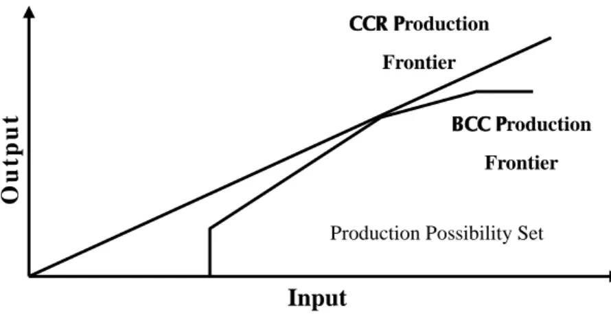
Figure 2.1 Production frontier of the CCR model 11
Figure 2.2 Production frontier of the BCC Model 11
Figure 3.1 The relationship between CCR model and BCC model 17
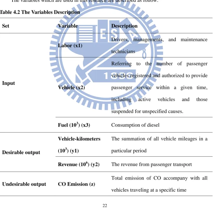
Figure 4.1 Trend of employees by year 25
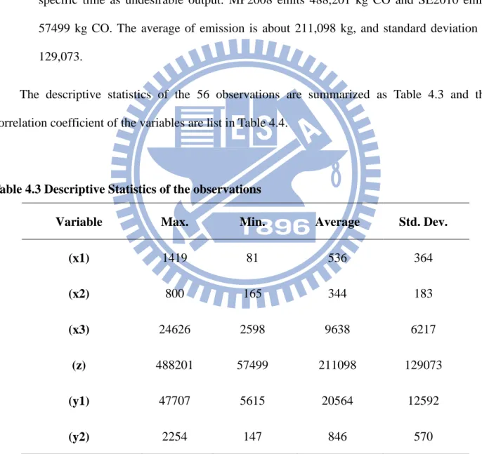
Figure 4.2 Trend of vehicles by Year 26
Figure 4.3 Trend of fuel consumptions by Year 26
Figure 4.4 Trend of vehicle-kms by Year 27
Figure 4.5 Trend of revenue by Year 27
Figure 4.6 Trend of COemissions by Year 28
Figure 4.7 Time trends of annual average of efficiency scores from 2007 to 2010, without and
with undesirable in the three scenarios 46
Figure 4.8 Average efficiency scores of the 14 firms for three scenarios 48
VII
List of Tables
Table 2.1 Summarization of bus transit efficiency research 7
Table 2.2 Summarization of bus transit efficiency research integrating undesirable output 9
Table 4.1 Current Companies of Taipei Bus System 21
Table 4.2 The Variables Description 22
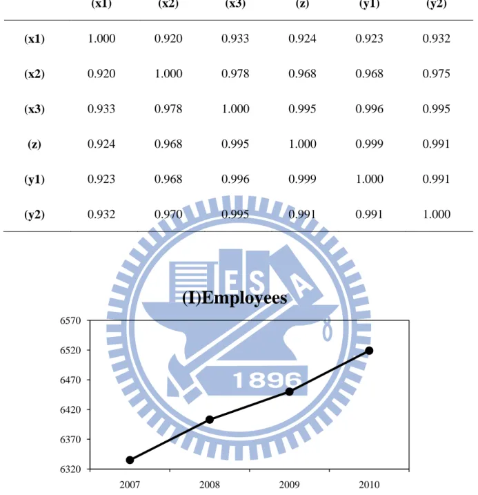
Table 4.3 Descriptive Statistics of the observations 24
Table 4.4 Correlation of the Variables 25
Table 4.5 Statistics on input and output data 29
Table 4.6 The results of considering without/ with undesirable outputs 29
Table 4.7 The score and rank without/with consideration of undesirable outputs 30
Table 4.8 Statistics on input/ output data 31
Table 4.9 Results of considering without/ with undesirable outputs 31
Table 4.10 The score and rank without/with consideration of undesirable outputs 32
Table 4.11 Statistics on input/ output data 33
Table 4.12 Results of considering without/ with undesirable outputs 34
Table 4.13 The score and rank without/with consideration of undesirable outputs 35
Table 4.14 Efficient DMUs without/with undesirable output from 2007 to 2010 36
Table 4.15 Slack analysis in scenario one 37
Table 4.16 Slack analysis in scenario two 40
Table 4.17 Slack analysis in scenario three 43
Table 4.18 Averages of efficiency scores in the three scenarios 47
Table 4.19 Potential input and output values 48
Table 4.20 Intermediate input expenditure and CO emission covering the period 2007-2010,
1
Chapter 1 Introduction
1.1 Motivation and background
Bus transit is one of the main public transportation all over the world. Due to the small
dimensionality, bus transit has become the most important transportation in Taiwan. However, as
the income growing, there are more and more private vehicles which significantly influenced the
demand of bus transit. Also the problems of the operating administration rose, such as great
employee expenses, inefficient production, and improper route managing, therefore the bus transit
operators sank to scrapes and can’t better the service level, bringing a vicious circle. Thus, the
operation of bus transit became difficult, and deficit appeared. The operational performance and
service quality went worse. The way to skip the bad condition is to find out the causes of
inefficiency and improve the efficiency.
Quantities of researches are proposed to measure performance, and Data Envelopment
Analysis (DEA) is a commonly used measure of efficiency. However, DEA usually assumes that
producing more outputs relative to less input resources is a criterion of efficiency (Cooper et al.,
2007). Producing the desirable outputs sometimes accompanies with undesirable outputs, such as
pollutions. Undesirable outputs damage the environments the properties, therefore inefficiency
arises. As the environmental issues are taken seriously, undesirable outputs should be taken into
the efficiency model, which urges the firms concern not only increasing good outputs but also
decreasing bad outputs.
A variety of opinions have been proposed in dealing with the undesirable outputs. A common
approach is to treat undesirable outputs as inputs (Lansink and Reinhard, 2004). As inefficient
firms want to improve performance, the objective is minimizing inputs and undesirable outputs.
However, treating undesirable outputs as inputs doesn’t reflect the true production process
2
emphasizes reducing undesirable outputs must accompany decrease in desirable outputs or
increase in inputs. That is to say, it needs cost to lessen undesirable outputs (Färe et al, 1989).
The purpose of this research is to investigate how undesirable outputs influence performance,
using the data of Taipei bus transit. The research is organized as follow: Chapter 2 reviews
literature on undesirable outputs and DEA; Chapter 3 explains the research methodology; Chapter
4 analyzes the research data; Chapter 5 discusses the results and Chapter 6 concludes and
recommends the research.
1.2 Research objectives and scope
Based on the motivation and background, the purposes of this research are as follows.
1. To Review and summarize the related papers in investigating how to deal with undesirable
outputs by different DEA models.
2. Using adjusted DEA model—Slacks-based measure of efficiency in DEA to analysis the data
to evaluate the efficiencies of different bus transit operators.
3. To give a recommendation to eliminate inefficiency and ameliorate performance.
1.3 Framework and procedures
3
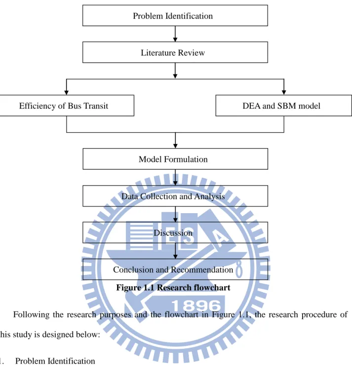
Figure 1.1 Research flowchart
Following the research purposes and the flowchart in Figure 1.1, the research procedure of
this study is designed below:
1. Problem Identification
Define the research target and scope and confirm the objectivities of this study. Furthermore,
determine the methodologies to resolve the problem.
2. Literature Review
Review the studies related to measuring the efficiency of bus transit, undesirable outputs, DEA,
and SBM model.
3. Model formulation
Conclusion and Recommendation Model Formulation
Data Collection and Analysis
Discussion
Efficiency of Bus Transit DEA and SBM model
Problem Identification
4
Based on the literatures, develop a multi objective programming model to evaluate performance.
4. Data Analysis
Analyze the inputs, desirable outputs and undesirable outputs to identify which operator is
efficient and which is inefficient.
5. Conclusions and Recommendations
Based on the results of analysis, to make conclusion and give recommendation to inefficient
5
Chapter 2 Literature Review
2.1 Measuring the efficiency of bus transit
There is a basic definition of efficiency which uses the relationship between input and output.
Labor, capital, and energy are three common input variables for measuring the efficiency of bus
transit. In the early studies, desirable outputs are generally used as the output variables to measure
the efficiency of bus transit, such as vehicle-kilometers, seat-kilometers, and
passenger-kilometers.
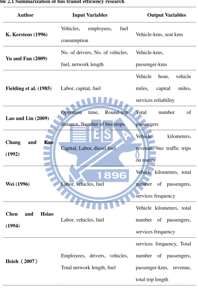
Kerstens (1996) measured the efficiency of French urban transit sector by using DEA and
FDH two methods. In this case, inputs are set as the number of vehicles, the number of employees,
and the fuel consumption, while outputs are presented by vehicle-kilometers and seat-kilometers.
The study confirmed the significance of the choice between deterministic nonparametric reference
technologies for technical efficiency measurement. However, this research cannot identify
whether DEA or FDH is better due to the lack of information.
Yu and Fan (2009) proposed a mixed structure network data envelopment analysis
(MSNDEA) model which can be used to simultaneously estimate the production efficiency,
service effectiveness and operational effectiveness of multimode transit firms. In this research,
inputs are the number of drivers, the number of vehicles, fuel, and network length, while outputs
are vehicle-kilometers, passenger-kilometers. This paper presents different results obtained from
MSNDEA model and conventional DEA model.
Fielding et al. (1985) analyzed the performance of bus transit in U.S. (based uses FY 1980
Section data 15) by using labor, capital, and fuel as input variables and using vehicle hour, vehicle
miles, capital miles, and services reliability as output variables. The objectives of this research are
6
capability, and testing the validity of the methodology developed from the previous analysis of FY
1979 data.
Lao and Liu (2009) combined DEA and geographic information systems (GIS) to examine
the operational efficiency and spatial effectiveness of a public transit system in Monterey-Salinas
area. Operation time, round-trip distance, and number of bus stops are used as inputs, and the
number of passengers is output. After evaluating the performance of bus line, this research
suggested ways to improve the performance of bus lines.
Kuo and Kao (1992) used DEA to measure the relative efficiency of public versus private
municipal bus forms in Taipei. Taipei Municipal Bus (TB) is publicly owned, while Hsin-Hsin,
Ta-Yao, Ta-Nan, and Kuang-Hua are privately owned. Data of the five bus firms in 1970-1988 are
adapted. Inputs include capital (the number of buses in operations), labor (the number of fulltime
employees), and diesel fuel. And outputs combine vehicle-kilometers, revenue and the number of
bus traffic trip on routes. The result shows TB had lower efficiency scores than the private firms.
7
Table 2.1 Summarization of bus transit efficiency research
Author Input Variables Output Variables
K. Kerstens (1996)
Vehicles, employees, fuel
consumption
Vehicle-kms, seat kms
Yu and Fan (2009)
No. of drivers, No. of vehicles,
fuel, network length
Vehicle-kms,
passenger-kms
Fielding et al. (1985) Labor, capital, fuel
Vehicle hour, vehicle
miles, capital miles,
services reliability
Lao and Liu (2009)
Operation time, Round-trip
distance, Number of bus stops
Total number of
passengers
Chang and Kao (1992)
Capital, Labor, diesel fuel
Vehicle kilometers,
revenue, bus traffic trips
on routes
Wei (1996) Labor, vehicles, fuel
Vehicle kilometers, total
number of passengers,
services frequency
Chen and Hsiao (1994)
Labor, vehicles, fuel
Vehicle kilometers, total
number of passengers,
services frequency
Hsieh(2007)
Employees, drivers, vehicles,
Total network length, fuel
services frequency, Total
number of passengers,
passenger-kms, revenue,
8
To economists, efficiency means obtaining the maximum of output that can be produced
under a given unit of input. In fact, bus transits produce not only beneficial outputs (such as
passenger-kilometers or vehicle-kilometers), but also undesirable outputs (such as vehicle
emissions or accidents). In the past two decades, the effects of undesirable outputs are
significantly recognized, and a number of researchers proposed to integrate undesirable outputs
into efficiency measurement models.
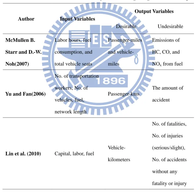
McMullen and Noh (2007) uses a directional distance function approach to demonstrate the
importance of considering reducing vehicular emissions as well as production of passenger or
vehicle-miles, when measuring agency efficiency. The analysis includes 43 single mode US bus
transit agencies for the year 2000. The emissions of HC, CO, and NOx from fuel are defined as
undesirable outputs which are simultaneously produced with transit outputs of vehicle- or
passenger-miles. The result shows that considering undesirable outputs changes the efficiency
score.
Yu and Fan (2006) employed the directional graph distance function and the multi-activity
data envelopment analysis (DEA) approach, which incorporates both desirable and undesirable
outputs, for the purpose of providing a more complete representation of the multimode bus
production technology from which environmentally and risk-sensitive cost effectiveness measures
can be generated. In order to make sense of wishing to decrease risky outputs, this research treats
accident cost as the risky output. This paper measures the cost effectiveness of 24 bus companies
in Taiwan, and indicates that the conventional DEA cost effectiveness measure may be seriously
misleading if it ignores the cost effectiveness of organizations that carry out various activities
whilst sharing common resources.
Lin et al. (2010) used stochastic frontier analysis (SFA) approach to analysis the data of ten
Taipei Bus Transit firms over 2001 to 2006 in order to investigate if the productive efficiency of a
9
by severity and correspond to different weighted score. The findings indicate that there exists
significant inefficiency in the Taipei bus transit industry as a whole. The productive efficiency
with adjustment of undesirable accidents is significantly different from that measured without
adjustment of accident effects.
Those studies are summarized as Table 2.2.
Table 2.2 Summarization of bus transit efficiency research integrating undesirable output
Author Input Variables
Output Variables Desirable Undesirable
McMullen B. Starr and D.-W. Noh(2007)
Labor hours, fuel
consumption, and
total vehicle seats
Passenger-miles and vehicle- miles Emissions of HC, CO, and NOx from fuel Yu and Fan(2006) No. of transportation workers, No. of vehicles, fuel, network length Passenger-kms The amount of accident
Lin et al. (2010) Capital, labor, fuel
Vehicle- kilometers No. of fatalities, No. of injuries (serious/slight), No. of accidents without any fatality or injury
10
2.2 Incorporating undesirable outputs in DEA
Data envelopment analysis (DEA) is an approach applied to measure multiple input-output
efficiency of decision making units (DMUs), which uses a linear programming based model.
Dealing with multiple input-output problem, the efficiency of DMUs are defined as follows:
outputs multiply relating weights and divided by inputs multiply relating weights. High relative
efficiency comes from high outputs and low inputs. That is to say, DEA uses inputs and outputs to
evaluate the efficiency of DMUs.
DEA is a non-parametric approach which means it doesn’t need assumption about the weight
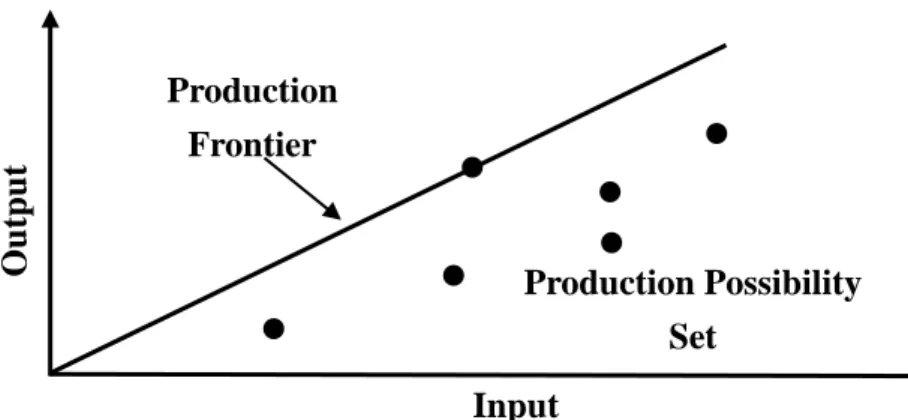
of the underlying production function. Farrell (1957) proposed frontier production function
method, using technical efficiency to measure productive efficiency. Given the input set, the
maximum output level is an efficient point. Link all the efficient points and become production
frontier. Every point on the production frontier is efficient, and other points under the frontier are
inefficient.
Based on the production frontier, Charnes et al. (1978) proposed CCR model to measure
efficiency under constant returns to scale. The DEA model is developed then. The DMUs on the
efficient frontier are those with maximum output level for given inputs or with minimum input
level for given outputs. Later Banker et al. (1984) proposed BCC model, adding a convexity
constraint to relax the assumptions of CCR model. BBC can evaluate multi inputs and outputs
11
Figure 2.1 Production frontier of the CCR model (adapted from Cooper, W.W., Seiford, L.M. and Tone, K., 2007. Data Envelopment Analysis: A Comprehensive Text with Models,
Applications, References and DEA-Solver Software)
Figure 2.2 Production frontier of the BCC Model (adapted from Cooper, W.W., Seiford, L.M. and Tone, K., 2007. Data Envelopment Analysis: A Comprehensive Text with Models,
Applications, References and DEA-Solver Software)
As Charnes et al. (1978) described, the classical DEA models rely on the assumption that
maximizing outputs and minimizing inputs. However, it’s not in accordance with current situation. Sometimes the production process may also generate by products which we don’t like, and it’s called undesirable outputs such as waste, water pollution or smoke pollution. Those undesirable
outputs have been reduced as possible to achieve the best efficiency, while traditional DEA model
supposes that outputs should be increased as more as possible. Apparently classical DEA model is Production Possibility Set Input Ou tpu t Production Frontier Production Possibility Set Input Ou tpu t Production Frontier
12
not suitable for dealing with undesirable outputs.
Cooper et al. (2007) classified DEA into four types— radial, non-radial and oriented,
non-radial and non-oriented, and radial and non-radial. Conventional DEA models are radial and
oriented, and they cannot take account the slackness of input and output. Thus, Tone (2001)
proposed a non-radial and non-oriented SBM model.
2.3 Incorporating undesirable outputs in SBM model
Based on slack variables, Tone (2001) proposed SBM model, using slack variables to
evaluate performance. The SBM model is non-radial and non-oriented, and directly utilizes input
and output slacks in producing an efficiency measure. The model provides the fully efficiency
score 1 to a DMU if and only if the DMU is efficient and gives a score less than 1 to inefficient
DMU.
Cooper et al. (2007) introduced a separable and non-separable inputs/outputs model. The
model extends to cope with co-existence of non-separable desirable and undesirable outputs.
Sometimes a certain bad outputs are closely related with a certain inputs, therefore reducing bad
outputs is accompanied by reducing good outputs. For instance, producing paper is accompanied
with water and air pollution, and electric industries emit Nitrogen Oxides (NOa) and Sulfur
Dioxides (SO2).
In this model, it proposed to decompose the set of good and bad outputs ( ) into ( )
and ( ) denote the separable good outputs, and non-separable good and bad outputs
respectively.
2.4 Summary
The issue which concerns about the performance of bus transit has been proposed in the past
13
cause external cost and may lead to a biased result.
In previous studies, labor, capital, and fuel are commonly used as input variable, vehicle-kms,
passengers, and revenue are desirable output variable, while accidents and emission are the
indicators of undesirable output.
With the advantage which can deal with separable and non-separable input/output, SBM
model which incorporates undesirable outputs (Cooper et al. 2007) will be used as the
14
Chapter 3 Methodology
3.1 The development of data envelopment analysis
DEA was developed as a method for evaluating the comparative efficiencies of DMUs, and it
can simultaneously consider multiple inputs and outputs. DEA can identify the benchmark
members of the efficient set and also identify these sources of inefficiency.
This approach was developed by Charnes et al. (1978) who extended the
single-output/single-input ratio to multiple-inputs / multiple-outputs. Based on the CCR model,
Banker et al. (1984) proposed a new model to estimate technical efficiency and scale inefficiency
in DEA by adding a convexity constrain. The BCC model relaxed the constant returns-to-scale
assumption to be variable returns-to-scale. Tone (2001) proposed a slack-based measure (SBM)
model to treat the slacks (the input excesses and output shortfalls) directly in the objective
function.
3.2 The CCR model
The CCR model is the basic DEA model. It can be used in CRS situation only. The original
model is showed in formula 3.1. The model assumes n DMUs, and each
utilizes m kinds of inputs and produces s kinds of outputs .
The efficiency of DMU k can be estimated by (3-1).
v u Max ,
m j jk j s r rk r k x v y u h 1 1 (3-1)15 s.t. 1 1 1
m j ji j s r ri r x v y u , i1,2,,n 0 j v , j1 ,2, ,m 0 r u , r 1,2,,sThen, Charnes et al. transform model (3-1) into linear problem to simplify the problem. The
linear model is as follows:
v u Max ,
s r rk r k u y h 1 s.t. 0 1 1
m j ji j s r ri ry v x u , i1,2,,n (3-2) 1 1
m j jk jx v , 0 j v , j1 ,2, ,m 0 r u , r 1,2,,sSince the number of constraints is greater than the number of variables, one can transform it
into dual problem as follows:
i z Min ,
z
s.t. 0 1
n i i ji jk x zx , j1 ,2, ,m (3-3)16 0 1
n i i ri rk y y , r1 ,2, ,s 0 i , i1,2,,nz is a scalar, which is the efficiency of kth firm, and it ranges from zero to unity. If z=1, the
firm is efficient. And if z is less than one, the firm is inefficient.
3.3 The BCC model
The CCR model is constructed under the assumption of CRS production technology.
However, production technology changes with environment or human factors in reality. Banker et
al. (1984) relaxed the CRS constraint to VRS technology by adding a convexity constraint, so that
the returns to scale of DMU can be separated to increasing, decreasing, and constant returns to
scale. The BCC input oriented model as follows:
i z Min ,
z
s.t. 0 1
n i i ji jk x zx , j1 ,2, ,m (3-4) 0 1
n i i ri rk y y , r1 ,2, ,s 0 i , i1,2,,n 1 1
n i i 17
Figure 3.1 The relationship between CCR model and BCC model (Adapted from Cooper, W.W., Seiford, L.M. and Tone, K., 2007. Data Envelopment Analysis: A Comprehensive
Text with Models, Applications, References and DEA-Solver Software)
3.4 The SBM model
Conventional DEA models evaluate performances by ratio efficiency which assumes that
there exists ratio between input and output. However the assumption is not suitable some
conditions. Tone (2001) proposed a slack-based measure (SBM) of efficiency in DEA. SBM
model deals directly with the input excesses and output shortfalls of the DMU concerned. The
following properties are satisfied by SBM model.
1. Units invariant: The measure should be invariant with respect to the units of data.
2. Monotone: The measure should be monotone decreasing in each slack in input and output.
3. Reference-set dependent: The measure should be determined only by consulting the
reference-set of the DMU concerned.
Describe the DMU ( ) as
(3-5) CCR Production Frontier BCC Production Frontier Input O u tp u t
18
(3-6)
and define an index as follows:
Min
(3-7)
with and
m and s are the number of input and output items; is a non-radial slack index and and
respectively stand for input excesses and output shortfalls. Multiply a scalar variable t (>0) to
both the denominator and the numerator of (3.7) which causes no change in .
Min (3-8)
s.t.
A DMU is SBM-efficient if . The condition is equivalent to and , i.e.,
no input excesses and no output shortfalls.
3.5 Non-separable ‘good’ and ‘bad’ output model
It is usually observed that bad outputs co-existence with good outputs. Cooper et al. (2007)
proposed to decompose the set of good and bad outputs. It is reasonable that the slacks in
non-separable (non-radial) bad outputs and non-separable inputs should affect the overall
efficiency, since even the radial slacks are sources of inefficiency. The following model is used to
19
(3-9) S.t.
Then decompose the inefficiency into respective inefficiencies as follows:
(3-10) Where
(Separable Input) (3-11)
20 (Non-Separable Input) (3-12) (3-13)
(Non-Separable Good Output) (3-14)
21
Chapter 4 Data Analysis
4.1 The data
As a developed public transport, Taipei bus transit is used as the case study in the thesis. In
the earlier periods, there was only one bus operator in Taipei, which belonged to Taipei City Bus
Administration, with 51routes and 651 buses. From 1969, the Taipei City Government opened
more opportunities to privately-owned firms for operating buses, including Shin-shin Bus, Air Bus,
Da-nan Bus, and Kuang-hua Bus, with 90 routes and 847 buses. Up until 1976, Taipei Bus System
included only a few private companies and was managed by the Taipei City Government.
Currently there are in total 14 privately-owned bus operators (listed on Table 4.1), serving
for almost seven-million people inhabited in Taipei metropolitan area. With 308 routes and 3,898
buses (until 2010 Dec.), these bus operators provided 243,900 thousand vehicle-kilometers and
carried 647,479 thousand passenger-trips in 2010.
Table 4.1 Current Companies of Taipei Bus System Companies
Metropolitan Bus (MP) Capital Bus (CP)
Shin-shin Bus (SS) Zhinan Bus (ZN)
Air Bus(AB) Chung-shing Bus (CS)
Da-nan Bus(DN) Xindian Bus (XD)
Kuang-hua Bus (KH) Southeast Bus (SE)
Taipei Bus (TP) Tanshui Bus (TS)
22
Following previous studies, several authors have studied the efficiency performance of bus
transit. Most of these studies utilized service inputs (such as labor, vehicle, and fuel) as input
variables, while utilized service outputs (such as vehicle hours, vehicle miles, and capacity miles)
and service consumption (such as passengers, passenger miles, and operating revenue) as
desirable output variables. On the other hand, bus transit industry produces several kinds of
undesirable outputs such as air pollution. Diesel is generally used as fuel in bus transit industry,
and there are several emissions from the buses, e.g., carbon monoxide (CO), hydrocarbon (HC),
nitrogen oxides (NOx), particulate matters (PM), which are causes for acid rain and smog.
The variables which are used in this research are described as follow:
Table 4.2 The Variables Description
Set Variable Description
Input
Labor (x1)
Drivers, managements, and maintenance
technicians
Vehicle (x2)
Referring to the number of passenger
vehicles registered and authorized to provide
passenger service within a given time,
including active vehicles and those
suspended for unspecified causes.
Fuel (103) (x3) Consumption of diesel
Desirable output
Vehicle-kilometers (103) (y1)
The summation of all vehicle mileages in a
particular period
Revenue (106) (y2) The revenue from passenger transport
Undesirable output CO Emission (z)
Total emission of CO accompany with all
23
The data used in this research is provided by Public Transportation Office in Taipei City.
Firms with incomplete data or unreasonable data are deleted. As such, two firms have been
excluded from this empirical analysis because of small scale of market share (less than 1% of all).
There are fourteen firms over a four-year horizon from 2007 to 2010. Totally, there are 48
observations (DMUs) in this research.
1. Input
(1) Labor: Drivers, managements, and maintenance technicians are included in labors.
The maximum number of labors is 1,419 in MP2010. The minimum number 81
shows at SE2007. The average of labor is about 536, and the standard deviation is
364.
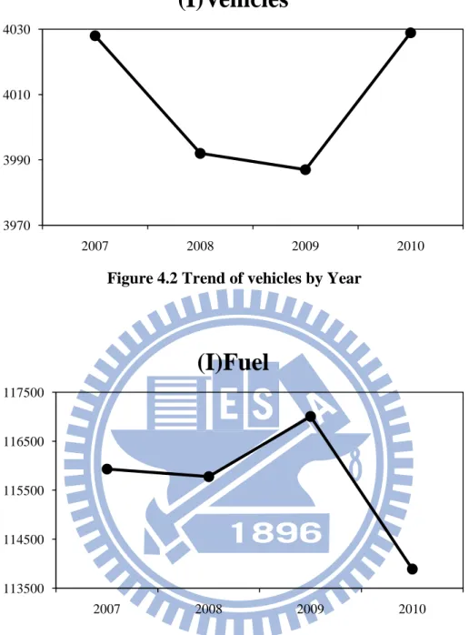
(2) Vehicle: The number of passenger or freight transport vehicles registered and
authorized to provide passenger service or freight delivery within a given time.
MP2010 has the most vehicle, 800, and AB2009 has the least number, 165. The
average of vehicle is about 344, and the standard deviation is 183.
(3) Fuel: The consumption of diesel is used as the variable. MP2007 consumes 24,626
kilo litre, being the maximum, while SE 2010 consumes 2598 kilo litre, being the
minimum. The average of fuel is about 9,638 kilo litre, and the standard deviation is
6,217.
2. Desirable output
(1) Vehicle-kms: The summation of all vehicle mileages in a particular period is
described as vehicle-kms. The maximum is 47,707 thousand vehicle-kms, MP2007;
while the minimum is 5615 thousand vehicle-kms, SE 2010. The average of
24
(2) Revenue: The revenue from passenger transport is defined as revenue. MP2008 has
the most revenue, 2,254 million NT dollar; while SE2009 has the least revenue, 147
million NT dollar. The average of revenue is about 846 million NT dollar, and the
standard deviation is 570.
3. Undesirable output
In this research we use total emission of CO accompany with all vehicles traveling at a
specific time as undesirable output. MP2008 emits 488,201 kg CO and SE2010 emits
57499 kg CO. The average of emission is about 211,098 kg, and standard deviation is
129,073.
The descriptive statistics of the 56 observations are summarized as Table 4.3 and the
correlation coefficient of the variables are list in Table 4.4.
Table 4.3 Descriptive Statistics of the observations
Variable Max. Min. Average Std. Dev.
(x1) 1419 81 536 364 (x2) 800 165 344 183 (x3) 24626 2598 9638 6217 (z) 488201 57499 211098 129073 (y1) 47707 5615 20564 12592 (y2) 2254 147 846 570
25 Table 4.4 Correlation of the Variables
(x1) (x2) (x3) (z) (y1) (y2) (x1) 1.000 0.920 0.933 0.924 0.923 0.932 (x2) 0.920 1.000 0.978 0.968 0.968 0.975 (x3) 0.933 0.978 1.000 0.995 0.996 0.995 (z) 0.924 0.968 0.995 1.000 0.999 0.991 (y1) 0.923 0.968 0.996 0.999 1.000 0.991 (y2) 0.932 0.970 0.995 0.991 0.991 1.000
Figure 4.1 Trend of employees by year 6320 6370 6420 6470 6520 6570 2007 2008 2009 2010
(I)Employees
26
Figure 4.2 Trend of vehicles by Year
Figure 4.3 Trend of fuel consumptions by Year 3970 3990 4010 4030 2007 2008 2009 2010
(I)Vehicles
113500 114500 115500 116500 117500 2007 2008 2009 2010(I)Fuel
27
Figure 4.4 Trend of vehicle-kms by Year
Figure 4.5 Trend of revenue by Year 242000 244000 246000 248000 250000 2007 2008 2009 2010
(O)Vehicle-kms(thousand)
9800 9900 10000 10100 10200 10300 10400 2007 2008 2009 2010(O)Revenue(million)
28
Figure 4.6 Trend of COemissions by Year
4.2 Empirical results
According to Fielding et al. (1985), there are two categories relating to desirable outputs—
service outputs, and service consumption. Therefore, in this section we set three scenarios to
estimate the efficiency scores with and without undesirable outputs respectively. In scenario one,
service output (vehicle-kms) is used as desirable output. In scenario two, service consumptions
(passengers and revenue) are used as desirable outputs. In scenario three, both service output and
service consumptions are discussed as desirable outputs.
4.2.1 Scenario one
This scenario discusses the relationship amount inputs, service outputs, and undesirable
outputs. 2500000 2510000 2520000 2530000 2540000 2550000 2007 2008 2009 2010
(OBad)CO Emissions
29 Table 4.5 Statistics on input and output data
Variable Max. Min. Average Std. Dev.
(x1) 1419 81 536 364
(x2) 800 165 334 183
(x3) 24626 2598 9638 6217
(z) 488201 57499 211098 129073
(y1) 47707 5615 20564 12592
We applied the SBM model and undesirable output model in Section 3.5 to the 48 DMUs
respectively, and got the scores and ranks as Table 4.6. As applying SBM model and considering
without undesirable outputs, there are 6 DMUs which meet ρ*=1, i.e. the 6 DMUs are efficient.
However, using undesirable output model with undesirable outputs, there are only 4 DMUs are
efficient. There are two firms become unefficient after consider undesirable outputs.
Table 4.6 The results of considering without/ with undesirable outputs
DMU
Without Undesirable Outputs With Undesirable Outputs
Score Rank Score Rank
AB 2007 1.000 1 1.000 1 XD 2007 1.000 1 1.000 1 SC 2008 1.000 1 1.000 1 XD 2008 1.000 1 0.945 10 SE 2008 1.000 1 0.856 19 SC 2009 1.000 1 1.000 1
30
Table 4.7 The score and rank without/with consideration of undesirable outputs
DMU
Without Undesirable Outputs With Undesirable Outputs 2007 2008 2009 2010 Av. Rank 2007 2008 2009 2010 Av. Rank MP 0.891 0.896 0.878 0.869 0.884 4 0.951 0.896 0.879 0.870 0.899 7 SS 0.797 0.818 0.806 0.809 0.807 7 0.802 0.825 0.813 0.768 0.802 6 AB 1.000 0.743 0.726 0.725 0.799 8 1.000 0.774 0.756 0.754 0.821 4 DN 0.849 0.676 0.674 0.682 0.720 10 0.876 0.704 0.709 0.710 0.750 9 KH 0.646 0.662 0.641 0.630 0.645 12 0.681 0.688 0.665 0.654 0.672 12 TP 0.983 0.966 0.971 0.931 0.963 2 0.989 0.987 0.973 0.935 0.971 3 SC 0.950 1.000 1.000 0.935 0.971 1 0.954 1.000 1.000 0.939 0.973 2 CP 0.848 0.836 0.836 0.831 0.838 6 0.853 0.840 0.839 0.832 0.841 5 ZN 0.739 0.741 0.733 0.703 0.729 9 0.772 0.774 0.745 0.729 0.755 8 CS 0.690 0.704 0.697 0.672 0.691 11 0.726 0.732 0.725 0.697 0.720 11 XD 1.000 0.945 0.938 0.946 0.957 3 1.000 1.000 0.990 0.996 0.997 1 SE 0.874 0.856 0.845 0.846 0.855 5 0.806 1.000 0.701 0.696 0.801 10 Av. 0.867 0.852 0.816 0.798 0.833 0.856 0.820 0.812 0.798 0.822 4.2.2 Scenario two
This scenario discusses the relationship amount inputs, service consumption, and undesirable
31 Table 4.8 Statistics on input/ output data
Variable Max. Min. Average Std. Dev.
(x1) 1419 18 536 364
(x2) 800 165 334 183
(x3) 24626 2598 9638 6217
(z) 488201 57499 211098 129073
(y2) 2254 147 846 570
The same as scenario one, we applied the SBM model and undesirable output model to
measure the efficiency with and without undesirable outputs respectively, and got the scores and
ranks as Table 4.9.
Table 4.9 Results of considering without/ with undesirable outputs
DMU
Without Undesirable Outputs With Undesirable Outputs
Score Rank Score Rank
XD 2007 1.000 1 1.000 1
SC 2008 1.000 1 1.000 1
AB 2010 1.000 1 1.000 1
32
Without considering undesirable outputs, there are 4 DMUs which meet ρ*=1, i.e. the 4
DMUs are efficient. With considering undesirable outputs, there are still 4 DMUs are efficient.
Table 4.10 The score and rank without/with consideration of undesirable outputs
DMU
Without Undesirable Outputs With Undesirable Outputs 2007 2008 2009 2010 Av. Rank 2007 2008 2009 2010 Av. Rank MP 0.921 0.961 0.912 0.919 0.928 4 0.930 0.982 0.922 0.935 0.942 5 SS 0.725 0.750 0.765 0.797 0.760 7 0.692 0.719 0.744 0.750 0.726 7 AB 0.612 0.907 0.975 1.000 0.873 5 0.553 0.848 0.973 1.000 0.844 4 DN 0.740 0.701 0.667 0.669 0.694 8 0.705 0.700 0.651 0.650 0.677 8 KH 0.586 0.592 0.573 0.547 0.575 12 0.551 0.554 0.536 0.506 0.537 11 TP 0.913 0.954 0.948 0.976 0.948 2 0.867 0.928 0.918 0.974 0.922 3 SC 0.924 1.000 0.947 0.918 0.947 3 0.910 1.000 0.933 0.908 0.938 2 CP 0.759 0.790 0.794 0.810 0.788 6 0.721 0.768 0.774 0.798 0.765 6 ZN 0.664 0.691 0.676 0.659 0.672 10 0.615 0.650 0.632 0.615 0.628 10 CS 0.670 0.683 0.664 0.675 0.673 9 0.649 0.660 0.637 0.664 0.652 9 XD 1.000 0.987 0.972 1.000 0.990 1 1.000 0.982 0.963 1.000 0.986 1 SE 0.580 0.647 0.688 0.706 0.655 11 0.347 0.360 0.354 0.358 0.355 12 Av. 0.758 0.805 0.798 0.806 0.792 0.712 0.763 0.753 0.763 0.748
33 4.2.3 Scenario three
This scenario discusses the relationship amount inputs, service outputs, service consumption,
and undesirable outputs.
Table 4.11 Statistics on input/ output data
Variable Max. Min. Average Std. Dev.
(x1) 1419 81 536 364 (x2) 800 165 344 183 (x3) 24626 2598 9638 6217 (z) 488201 57499 211098 129073 (y1) 47707 5615 20564 12592 (y2) 2254 147 846 570
The same as previous one, we applied the SBM model and undesirable output model to
measure the efficiency with and without undesirable outputs respectively, and got the scores and
ranks as Table 4.11.
Without considering undesirable outputs, there are 11 DMUs which meet ρ*=1, i.e. the 11
DMUs are efficient. With considering undesirable outputs, there are only 7 DMUs are efficient.
34
Table 4.12 Results of considering without/ with undesirable outputs
DMU
Without Undesirable Outputs With Undesirable Outputs
Score Rank Score Rank
MP 2007 1.000 1 0.912 18 AB 2007 1.000 1 1.000 1 XD 2007 1.000 1 1.000 1 AB 2008 1.000 1 1.000 1 SC 2008 1.000 1 1.000 1 XD 2008 1.000 1 0.987 8 SE 2008 1.000 1 0.742 32 AB 2009 1.000 1 0.972 13 SC 2009 1.000 1 1.000 1 AB 2010 1.000 1 1.000 1 XD 2010 1.000 1 1.000 1
35
Table 4.13 The score and rank without/with consideration of undesirable outputs
DMU
Without Undesirable Outputs With Undesirable Outputs 2007 2008 2009 2010 Av. Rank 2007 2008 2009 2010 Av. Rank MP 0.912 0.941 0.902 0.904 0.915 5 1.000 0.990 0.952 0.975 0.979 6 SS 0.767 0.789 0.790 0.809 0.789 7 0.776 0.798 0.797 0.781 0.788 8 AB 1.000 1.000 0.972 1.000 0.993 1 1.000 1.000 1.000 1.000 1.000 1 DN 0.896 0.704 0.676 0.681 0.739 9 0.900 0.712 0.701 0.696 0.752 9 KH 0.621 0.631 0.611 0.591 0.613 12 0.650 0.651 0.629 0.612 0.635 12 TP 0.977 0.979 0.979 0.977 0.978 3 0.982 0.984 0.981 0.978 0.981 3 SC 0.939 1.000 1.000 0.928 0.967 4 0.943 1.000 1.000 0.932 0.969 4 CP 0.806 0.815 0.817 0.822 0.815 6 0.817 0.821 0.823 0.824 0.821 7 ZN 0.706 0.722 0.709 0.686 0.706 10 0.731 0.746 0.721 0.702 0.725 10 CS 0.686 0.699 0.685 0.680 0.687 11 0.711 0.715 0.703 0.691 0.705 11 XD 1.000 0.987 0.964 1.000 0.988 2 1.000 1.000 0.986 1.000 0.997 2 SE 0.708 0.742 0.766 0.777 0.748 8 0.883 1.000 0.817 0.816 0.879 5 Av. 0.835 0.834 0.823 0.821 0.828 0.866 0.868 0.842 0.834 0.853 4.2.4 Summary
In section 4.2, three scenarios are introduced under considering service outputs, service
consumptions, or overall outputs respectively. The results are compiled and separate according to
36
in 2007 than in other years.
In scenario 1, service output (vehicle-kms) is used as output variable. There are 12 DMUs
efficient as consider without undesirable output; while only 4 DMUs are efficient if undesirable
output is involved. In scenario 2, service consumption (passengers and revenue) is the output
variable. There are 10 efficient DMUs under considering without undesirable output. If taking
undesirable output into account, there are 4 DMUs which are efficient. In scenario 3, both service
output and service consumption are involved in the model. There are 18 efficient DMUs and 6
efficient DMUs respectively as considering without and with undesirable output.
According to the results, over half of DMUs which are efficient as considering undesirable
output are not efficient if considering it.
Table 4.14 Efficient DMUs without/with undesirable output from 2007 to 2010
Scenario 1 Scenario 2 Scenario 3
2007
Without AB, XD XD MP, AB, XD
With AB, XD XD AB, XD
2008 Without SC, XD, SE SC AB, SC, XD, SE With SC SC AB, SC 2009 Without SC AB, SC With SC SC 2010
Without AB, XD AB, XD
With AB,XD AB, XD
Total
Without 6 4 11
37
4.3 Slack analysis
The DMUs have already classified as efficiency or inefficiency. To improve the inefficient
DMUs, slack values for the factors are computed. According to the three scenarios, we have
different results of slack analysis. The following analyses take undesirable output into account.
Table 4.15 Slack analysis in scenario one
DMU Score (x1) (x2) (x3) (y1) (z)
MP 2007 0.951 75.631 41.484 1002.496 0.000 0.000 SS 2007 0.802 376.680 5.089 764.335 0.000 0.000 AB 2007 1.000 0.000 0.000 0.000 0.000 0.000 DN 2007 0.876 124.908 0.000 0.000 0.000 0.000 KH 2007 0.681 273.175 75.821 0.000 0.000 0.000 TP 2007 0.989 15.822 2.112 0.000 0.000 0.000 SC 2007 0.954 74.387 0.000 689.849 0.000 0.000 CP 2007 0.853 255.998 54.417 581.711 0.000 0.000 ZN 2007 0.772 294.553 0.000 18.771 0.000 0.000 CS 2007 0.726 242.897 32.551 0.000 0.000 0.000 XD 2007 1.000 0.000 0.000 0.000 0.000 0.000 SE 2007 0.806 17.065 63.882 0.000 0.000 0.000 MP 2008 0.896 136.073 110.557 1764.523 0.000 0.000 SS 2008 0.825 367.686 0.000 249.684 0.000 0.000
38 Table 4.15 Slack analysis in scenario one (continued)
AB 2008 0.774 142.895 20.084 0.000 0.000 0.000 DN 2008 0.704 229.447 42.501 6.720 0.000 0.000 KH 2008 0.688 305.620 55.998 5.097 0.000 0.000 TP 2008 0.987 19.502 0.000 23.577 0.000 0.000 SC 2008 1.000 0.000 0.000 0.000 0.000 0.000 CP 2008 0.840 259.103 74.695 848.379 0.000 0.000 ZN 2008 0.774 288.846 0.000 83.247 0.000 0.000 CS 2008 0.732 265.099 18.631 0.113 0.000 0.000 XD 2008 1.000 0.000 0.000 0.000 0.000 0.000 SE 2008 1.000 0.000 0.000 0.000 0.000 0.000 MP 2009 0.879 167.316 132.031 1817.272 0.000 0.000 SS 2009 0.813 388.235 9.663 4.262 0.000 0.000 AB 2009 0.756 186.725 5.265 113.567 0.000 0.000 DN 2009 0.709 230.949 36.499 50.910 0.000 0.000 KH 2009 0.665 317.312 66.889 60.734 0.000 0.000 TP 2009 0.973 29.164 0.000 375.541 0.000 0.000 SC 2009 1.000 0.000 0.000 0.000 0.000 0.000 CP 2009 0.839 248.127 77.748 1036.474 0.000 0.000 ZN 2009 0.745 324.270 0.000 133.711 0.000 0.000
39 Table 4.15 Slack analysis in scenario one (continued)
CS 2009 0.725 268.431 20.452 53.198 0.000 0.000 XD 2009 0.990 1.372 1.104 58.054 0.000 0.000 SE 2009 0.701 33.500 83.123 27.689 0.000 0.000 MP 2010 0.870 198.843 139.841 1796.582 0.000 0.000 SS 2010 0.768 278.267 74.184 0.000 0.000 29840.976 AB 2010 0.754 178.012 7.819 120.081 0.000 0.000 DN 2010 0.710 232.243 37.067 26.804 0.000 0.000 KH 2010 0.654 326.673 78.807 0.000 0.000 0.000 TP 2010 0.935 67.019 24.236 295.216 0.000 0.000 SC 2010 0.939 98.726 0.000 932.244 0.000 0.000 CP 2010 0.832 247.230 93.779 1007.299 0.000 0.000 ZN 2010 0.729 351.962 4.229 37.637 0.000 0.000 CS 2010 0.697 289.381 34.894 16.668 0.000 0.000 XD 2010 0.996 0.292 0.575 24.641 0.000 0.000 SE 2010 0.696 35.974 83.852 6.946 0.000 0.000
40 Table 4.16 Slack analysis in scenario two
DMU Score (x1) (x2) (x3) (y2) (z)
MP 2007 0.930 96.695 77.662 2174.209 0.000 0.000 SS 2007 0.692 318.858 83.757 943.437 0.000 0.000 AB 2007 0.553 169.952 116.208 0.000 0.000 18539.951 DN 2007 0.705 226.472 39.288 0.000 0.000 10666.941 KH 2007 0.551 320.792 90.568 0.000 0.000 1836.989 TP 2007 0.867 0.000 74.917 36.235 0.000 0.000 SC 2007 0.910 112.663 7.655 622.780 0.000 0.000 CP 2007 0.721 359.211 87.396 438.130 0.000 0.000 ZN 2007 0.615 207.076 33.149 0.000 0.000 3127.647 CS 2007 0.649 277.016 36.764 0.000 0.000 1650.983 XD 2007 1.000 0.000 0.000 0.000 0.000 0.000 SE 2007 0.347 48.972 114.538 0.000 0.000 539.749 MP 2008 0.982 47.804 53.183 1387.831 0.000 0.000 SS 2008 0.719 310.500 76.380 496.371 0.000 0.000 AB 2008 0.848 158.384 16.836 0.000 0.000 4494.991 DN 2008 0.700 230.448 43.392 0.000 0.000 201.169 KH 2008 0.554 322.244 85.026 0.000 0.000 299.691 TP 2008 0.928 0.000 34.103 142.867 0.000 0.000
41 Table 4.16 Slack analysis in scenario two (continued)
SC 2008 1.000 0.000 0.000 0.000 0.000 0.000 CP 2008 0.768 317.900 93.460 753.641 0.000 0.000 ZN 2008 0.650 195.531 27.041 0.000 0.000 2337.869 CS 2008 0.660 272.672 31.588 0.000 0.000 408.281 XD 2008 0.982 1.836 2.294 0.000 0.000 334.170 SE 2008 0.360 51.380 115.270 0.000 0.000 80.712 MP 2009 0.922 122.336 101.729 1708.532 0.000 0.000 SS 2009 0.744 307.984 76.866 292.983 0.000 0.000 AB 2009 0.973 13.234 0.000 0.000 0.000 99.465 DN 2009 0.651 237.956 49.274 34.332 0.000 0.000 KH 2009 0.536 332.936 94.444 32.773 0.000 0.000 TP 2009 0.918 0.000 35.374 251.586 0.000 0.000 SC 2009 0.933 37.605 0.000 982.627 0.000 0.000 CP 2009 0.774 301.863 94.895 941.250 0.000 0.000 ZN 2009 0.632 203.245 29.619 0.000 0.000 1620.675 CS 2009 0.637 277.916 36.614 32.584 0.000 0.000 XD 2009 0.963 3.448 4.392 36.562 0.000 0.000 SE 2009 0.354 53.012 118.198 8.899 0.000 0.000 MP 2010 0.935 130.302 94.706 1547.466 0.000 0.000
42 Table 4.16 Slack analysis in scenario two (continued)
SS 2010 0.750 296.337 74.405 0.000 0.000 32642.869 AB 2010 1.000 0.000 0.000 0.000 0.000 0.000 DN 2010 0.650 238.732 47.878 9.327 0.000 0.000 KH 2010 0.506 347.240 109.260 0.000 0.000 527.946 TP 2010 0.974 0.000 26.564 185.879 0.000 0.000 SC 2010 0.908 117.632 8.627 902.020 0.000 0.000 CP 2010 0.798 276.211 101.196 932.408 0.000 0.000 ZN 2010 0.615 225.076 38.949 0.000 0.000 1589.181 CS 2010 0.664 293.100 40.950 0.000 0.000 44.087 XD 2010 1.000 0.000 0.000 0.000 0.000 0.000 SE 2010 0.358 54.808 117.832 0.000 0.000 95.649
43 Table 4.17 Slack analysis in scenario three
DMU Score (x1) (x2) (x3) (y1) (y2) (z)
MP 2007 1.000 0.000 0.000 0.000 0.000 0.000 0.000 SS 2007 0.776 246.831 63.094 1146.642 0.000 89.676 0.000 AB 2007 1.000 0.000 0.000 0.000 0.000 0.000 0.000 DN 2007 0.900 67.041 23.221 0.000 0.000 0.000 0.000 KH 2007 0.650 273.813 76.641 0.000 0.000 54.658 0.000 TP 2007 0.982 15.843 2.627 0.000 0.000 22.977 0.000 SC 2007 0.943 76.415 0.000 679.678 0.000 38.580 0.000 CP 2007 0.817 260.963 55.250 563.631 0.000 132.274 0.000 ZN 2007 0.731 296.949 0.111 0.000 0.000 61.901 0.000 CS 2007 0.711 243.160 32.902 0.000 0.000 23.258 0.000 XD 2007 1.000 0.000 0.000 0.000 0.000 0.000 0.000 SE 2007 0.883 4.801 17.353 0.000 0.000 31.400 0.000 MP 2008 0.990 15.849 7.787 195.418 0.000 0.000 0.000 SS 2008 0.798 244.161 55.175 609.254 0.000 88.057 0.000 AB 2008 1.000 0.000 0.000 0.000 0.000 0.000 0.000 DN 2008 0.712 222.505 42.162 0.549 0.000 0.000 0.000 KH 2008 0.651 306.185 56.997 0.000 0.000 70.780 0.000 TP 2008 0.984 19.975 0.000 22.331 0.000 9.946 0.000
44
Table 4.17 Slack analysis in scenario three (continued)
SC 2008 1.000 0.000 0.000 0.000 0.000 0.000 0.000 CP 2008 0.821 261.684 75.269 840.580 0.000 73.697 0.000 ZN 2008 0.746 291.263 0.000 72.124 0.000 44.138 0.000 CS 2008 0.715 265.343 19.067 0.000 0.000 27.814 0.000 XD 2008 1.000 0.000 0.000 0.000 0.000 0.000 0.000 SE 2008 1.000 0.000 0.000 0.000 0.000 0.000 0.000 MP 2009 0.952 76.037 56.353 456.246 0.000 0.000 0.000 SS 2009 0.797 265.393 63.772 360.783 0.000 55.229 0.000 AB 2009 1.000 0.000 0.000 0.000 0.000 0.000 0.000 DN 2009 0.701 231.063 36.704 50.853 0.000 12.678 0.000 KH 2009 0.629 317.746 67.632 44.625 0.000 70.493 0.000 TP 2009 0.981 21.877 0.000 32.888 0.000 15.309 0.000 SC 2009 1.000 0.000 0.000 0.000 0.000 0.000 0.000 CP 2009 0.823 250.461 78.282 1029.294 0.000 67.201 0.000 ZN 2009 0.721 326.030 0.000 122.506 0.000 37.443 0.000 CS 2009 0.703 268.708 20.936 48.357 0.000 37.555 0.000 XD 2009 0.986 1.262 0.876 43.457 0.000 7.059 0.000 SE 2009 0.817 14.176 33.517 19.616 0.000 29.400 0.000 MP 2010 0.975 56.105 27.184 0.000 0.000 0.000 0.000
45
Table 4.17 Slack analysis in scenario three (continued)
SS 2010 0.781 266.132 80.400 0.000 0.000 1.623 29886.186 AB 2010 1.000 0.000 0.000 0.000 0.000 0.000 0.000 DN 2010 0.696 232.401 37.339 22.391 0.000 23.662 0.000 KH 2010 0.612 327.356 79.991 0.000 0.000 75.480 0.000 TP 2010 0.978 11.348 17.707 126.837 0.000 0.000 0.000 SC 2010 0.932 95.895 1.829 940.963 0.000 26.374 0.000 CP 2010 0.824 248.558 93.926 1001.033 0.000 32.761 0.000 ZN 2010 0.702 352.153 4.536 20.863 0.000 44.082 0.000 CS 2010 0.691 289.381 34.873 7.035 0.000 12.867 0.000 XD 2010 1.000 0.000 0.000 0.000 0.000 0.000 0.000 SE 2010 0.816 15.366 33.295 0.000 0.000 29.600 0.000
4.4 Discussion
This study was designed to measure the operation efficiency of bus transit with consideration
of undesirable output and compare with the efficiency without considering undesirable output.
The findings indicate that many efficiency DMUs become inefficiency if involving undesirable
output into the DEA model. Therefore, ignoring undesirable outputs may cause bias in evaluation
of efficiency.
Figure 4.7 displays the trends of six average efficiency scores over time, without and with
undesirable output in the three scenarios, indicating the following: (1) in the three scenario, the
46
estimated with undesirable output; (2) the efficiency scores in scenario one and scenario three are
higher than the scores in scenario two; (3) the efficiency scores in scenario three are steadier than
those in scenario one and two. The above time trends show: (1) the efficiency scores are
overestimated under considering without undesirable output; (2) the efficiency scores are steadier
as both service outputs and service consumption are involved in the model.
Figure 4.7 Time trends of annual average of efficiency scores from 2007 to 2010, without and with undesirable in the three scenarios
Table 4.18 summarizes the average efficiency scores of the 12 firms from 2007 to 2010 in
the three scenarios. The table shows that in scenario three, AB hasρ*=1, being the most efficient
firm. Following are MP, TP, SC, and XD haveρ*>0.95, which means the four firms are
respectively efficient to others. Those efficient firms totally operating 992,956 thousand vehicle-
kms (55% of total) and carrying 2,567,696 thousand passengers (57% of total) in the period of
2007-2010. The operational universalities of the five efficiency firms are (1) (y1) > 10,000; (2)
(y2) > 30,000; (3) (y3)> 500, which indicate that the scales of firms have relationship with the
efficiency. 0.7 0.75 0.8 0.85 0.9 0.95 1 2007 2008 2009 2010 Scenario 1 (without) Scenario 2 (without) Scenario 3 (without) Scenario 1 (with) Scenario 2 (with) Scenario 3 (with)
47
Table 4.18 Averages of efficiency scores in the three scenarios
Firm Scenario 1 Scenario 2 Scenario 3
MP 0.899 0.942 0.979 SS 0.802 0.726 0.788 AB 0.821 0.844 1.000 DN 0.750 0.677 0.752 KH 0.672 0.537 0.635 TP 0.971 0.922 0.981 SC 0.973 0.938 0.969 CP 0.841 0.765 0.821 ZN 0.755 0.628 0.725 CS 0.720 0.652 0.705 XD 0.997 0.986 0.997 SE 0.801 0.355 0.879 Average 0.833 0.748 0.853
48
Figure 4.8 Average efficiency scores of the 14 firms for three scenarios
Based on the results, target values of the variables are provided. The following is the
potential input and output values in scenario three. According to the potential values, the DMUs
can improve the efficiency by increasing desirable outputs and decreasing inputs and undesirable
output.
Table 4.19 Potential input and output values
DMU Score (x1) (x2) (x3) (y1) (y2) (z)
MP 2007 1 1389 785 24626 2189 47707 488045 SS 2007 1 477 333 11186 1071 25367 259782 AB 2007 1 254 267 4720 412 12111 123923 DN 2007 1 268 211 5602 532 13104 134088 KH 2007 1 139 179 5445 507 11942 122241 0.000 0.100 0.200 0.300 0.400 0.500 0.600 0.700 0.800 0.900 1.000 MP SS AB DN KH TP SC CP ZN CS XD SE
Average efficiency
Scenario1 Scenario2 Scenario349
Table 4.19 Potential input and output values (continued)
TP 2007 1 514 509 15192 1280 33411 341870 SC 2007 1 729 414 14472 1407 33238 340105 CP 2007 1 654 394 13579 1316 31050 317704 ZN 2007 1 135 174 5282 495 11550 118216 CS 2007 1 125 167 5051 469 11062 113232 XD 2007 1 89 169 5127 458 11237 115699 SE 2007 1 76 155 3051 188 6673 68309 MP 2008 1 1371 783 23863 2254 47699 488196 SS 2008 1 485 338 11308 1087 25600 261999 AB 2008 1 251 183 4271 454 9586 98200 DN 2008 1 107 180 5259 488 11366 116300 KH 2008 1 116 207 6064 560 13113 134196 TP 2008 1 504 502 15029 1301 32523 332753 SC 2008 1 807 414 14827 1450 34317 351093 CP 2008 1 700 409 14187 1377 32523 332756 ZN 2008 1 144 177 5396 505 11838 121138 CS 2008 1 106 189 5535 510 11980 122607 XD 2008 1 102 182 5325 491 11520 117870 SE 2008 1 83 172 2825 155 6116 62490
50
Table 4.19 Potential input and output values (continued)
MP 2009 1 1317 739 23327 2159 47111 482040 SS 2009 1 460 329 10967 1052 24789 253725 AB 2009 1 276 165 4795 507 10134 103720 DN 2009 1 101 181 5194 474 11237 114973 KH 2009 1 110 197 5790 536 12502 127955 TP 2009 1 505 505 15350 1311 32979 337543 SC 2009 1 806 414 16023 1419 34384 351808 CP 2009 1 716 414 14391 1397 33014 337772 ZN 2009 1 111 176 5349 487 11715 120340 CS 2009 1 105 188 5507 509 11906 121837 XD 2009 1 102 182 5343 495 11536 118073 SE 2009 1 69 138 2605 176 5626 57599 MP 2010 1 1363 773 23639 2184 46986 480775 SS 2010 1 457 313 10628 1012 24196 248020 AB 2010 1 267 167 4794 514 10120 103588 DN 2010 1 102 181 5314 491 11488 117558 KH 2010 1 110 190 5595 515 12127 124120 TP 2010 1 521 489 14470 1314 31387 321200 SC 2010 1 711 412 14327 1390 32864 336230