國
立
交
通
大
學
多媒體工程研究所
碩
士
論
文
用於分層串流之同步滑動無限制比率碼:模型化及最佳化
Synchronized Sliding Window Rateless Coding for Layered Streaming:
Modeling and Optimization
研 究 生:邱詠智
指導教授:蕭旭峯 教授
用於分層串流之同步滑動無限制比率碼:模型化及最佳化
Synchronized Sliding Window Rateless Coding
for Layered Streaming: Modeling and Optimization
研 究 生:邱詠智 Student:Yong-Jhih Ciou
指導教授:蕭旭峯 Advisor:Hsu-Feng Hsiao
國 立 交 通 大 學
多 媒 體 工 程 研 究 所
碩 士 論 文
A ThesisSubmitted to Institute of Multimedia Engineering College of Computer Science
National Chiao Tung University in partial Fulfillment of the Requirements
for the Degree of Master
in
Computer Science September 2011
Hsinchu, Taiwan, Republic of China
i
用於分層串流之同步滑動無限制比率碼:模型化及最佳化
學生:
邱詠智指導教授:
蕭旭峯 博士國立交通大學多媒體工程研究所
摘 要
在異質網路中, 伺服器端必須傳送不同的串流檔案給不同需求的客戶端。但相同的檔案 必須準備不同串流,的這對伺服器端是一種很重的負擔。如果這時候我們可以將一個串流分 割成數個部分,而客戶端的使用者只要接收他們所需的部分的話,這將大大的減少伺服器端 的負擔。而這種方法就是「可調式視訊編碼」。 在現實的網路環境中,封包的遺失或損壞是不可避免的。當封包遺失或損壞時,重傳是 最一般的做法。但是,在某些環境中重傳是不被允許的。因此,我們必須嘗試使用已經接收 到的封包去回復這些有問題的封包,這種方法叫做「通道編碼」,而「噴泉編碼」也其中一種 通道編碼。 在本篇論文中,我們將會研究如何整合可調式視訊編碼和噴泉編碼,同時提供「非相等錯 誤保護」,保護可調式視訊編碼串流中比較重要的部分。此外我們還提出了兩個預測的模組。 其中一個模組是用來預測在我們提出的保護方法中,訊息區塊解碼失敗的機率是多少。而另 一個預測模組是預測在可調式視訊編碼解碼結束後有多少張圖可以成功的撥放出來。藉由使 用這兩個模組,最終我們可以產生擁有最大 PSNR 值的最佳化串流。ii
Synchronized Sliding Window Rateless Coding
for Layered Streaming: Modeling and Optimization
Student:Yong-Jhih Ciou Advisors:Dr. Hsu-Feng Hsiao
Institute of Multimedia Engineering
College of Computer Science
National Chiao Tung University
ABSTRACT
In heterogeneous networks, the server transports the streaming to the clients that have different requirement. It is a heavy load that the server has to prepare the different streaming for the same video. If we can cut a streaming into several parts, and the client users can receive the parts according to their requirement. It can reduce the load of server. The method is named SVC (Scalable Video Coding).
In real network environment, packet loss or damage is unavoidable. When packet loss or damage takes place, retransmission is one of the usual solutions. But, retransmission is not allowed in some environment. Therefore, we have to try to use the packets that we already receive to recovery the lost packets. The method can be done through “channel coding”, and the fountain codes is one kind of the channel coding approaches.
In this paper, we are going to research on the integration of SVC and Rateless codes. Meanwhile, unequal error protection scheme will be proposed to protect the important part of SVC streaming. In addition, we will propose two prediction models. One of the prediction models estimates the decoding failure probability of each message block in our proposed protection method. Another prediction model estimates the amount of frames that can be displayed successfully after SVC decoding. By using these two models, we finally can produce the optimized streaming that has the highest PSNR.
iii
誌
誌
謝
謝
首先我要感謝 蕭旭峯 老師兩年來的栽培和指導,讓我在就讀研究所的過程中不僅僅只是 學習到做研究的方法,也學習到正確的待人處事之道。接著我還要感謝同學蔣育叡、王以安 和李宗熹,因為有你們,讓我在學習的道路上並不孤單,我們曾經一起共患難,一起歡樂的 時光都成為我人生當中最美好的回憶。當然不能不提到學長董昀修、陳德沛、學弟黃志隆和 PSP LAB 的許瀚文和潘俊宇,在我遇到困難的時候,你們總是能即時的伸出援手提供我寶貴的 意見和想法,使得我可以順利的將問題迎刃而解。此外我要感謝我的父母和家人無微不至的 照顧,讓我在讀書的過程中沒有後顧之憂,可以全心全意的投入學習。因為有你們所以才能 造就現在的我,千言萬語都難以表達我內心的感激之意,真的非常感謝大家,謝謝。iv
C
C
o
o
n
n
t
t
e
e
n
n
t
t
s
s
摘 要 ... i ABSTRACT ... ii 誌 誌 謝謝 ... iii C Coonntteennttss ... iv L LiissttooffFFiigguurreess ... v L LiissttooffTTaabbllees ... vii s C Chhaapptteerr11::IInnttrroodduuccttiioonn ... 1 C Chhaapptteerr22::BBaacckkggrroouunnd ... 4 d 2.1 LT Codes... 4 2.2 Sliding Window ... 8 2.3 SVC ... 112.4 And-Or Tree Analysis ... 14
C Chhaapptteerr33::RReellaatteeddWWoorrkks ... 16 s 3.1 Expanding Window Fountain ... 16
3.2 The UEP Method of “Rateless Codes With Unequal Error Protection Property” [11] 18 3.3 The UEP Method of “Unequal Error Protection Using Fountain Codes with Applications to Video Communication” [12] ... 20
C Chhaapptteerr44::PPrrooppoosseeddMMeetthhood ... 22 d 4.1Proposed Synchronized Sliding Window Rateless Codes ... 22
4.2 Prediction Model ... 25
4.2.1 The probability that a level i AND-node will pass the 0 to the level i OR-node . 25 4.2.2 The probability that a level i OR-node will pass 0 to a level i+1 AND-node ... 27
4.2.3 To simplify ... 30
4.3 Selecting Best Weight ... 32
C Chhaapptteerr55::TThheeEExxppeerriimmeennttRReessuullttss ... 35
5.1 Accuracy Analysis for SSW Rateless Codes Model... 35
5.2 Confirm Relationship of PSNR and Total Displayed Frames ... 41
5.3 SSW on SVC Streaming Environment ... 44
5.4 SSW on SVC Streaming with Variable Bandwidth Environment ... 49
5.5 Performance of the Proposed Model with Robust Soliton Distribution ... 52
C Chhaapptteerr66::CCoonncclluussiioonn ... 54 R Reeffeerreennccees ... 55 s A AppppeennddiixxA ... 57 A
v
L
L
i
i
s
s
t
t
o
o
f
f
F
F
i
i
g
g
u
u
r
r
e
e
s
s
Fig. 1 Heterogeneous networks... 1
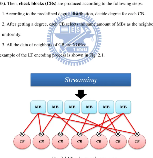
Fig. 2.1 LT codes encoding process ... 4
Fig. 2.2 Bad degree distribution example ... 6
Fig. 2.3 Overhead-number of MB graph ... 7
Fig. 2.4 Data partition ... 8
Fig. 2.5 Sliding Window encoding process ... 9
Fig. 2.6 Different types of SVC [15] ... 11
Fig. 2.7 SVC 4 Layer encoding example ... 12
Fig. 3.1 Encoding process of EWF ... 17
Fig. 3.2 The deviation of [11] with overhead: 0.04~0.2 and the step size=0.02,n=2000 ,kM=1~3 and total section=11 ... 20
Fig. 3.3 Example of encoding process of [12] with n0=2, n1=1, RF0=2, RF1=1 and EF=2 ... 21
Fig. 4.1 The content of each window in sliding window ... 23
Fig. 4.2 The data order of proposed method in each section ... 23
Fig. 4.3 Example of N-Cycle sliding of SSW on 4 layer input data and the content of each window ... 24
Fig. 4.4 The way of connection of a AND-node in AND-OR tree ... 25
Fig. 4.5 Pj ... 27
Fig. 4.6 Example of connection way of OR-node ... 28
Fig. 4.7 The example of layer 3 MBs are covered by 4 windows when N=4 ... 29
Fig. 4.8 Displaying the different amount of frames video ... 32
Fig. 4.9 The encoding Structure of SVC streaming ... 33
Fig. 4.10 The Dependence of SVC frame ... 33
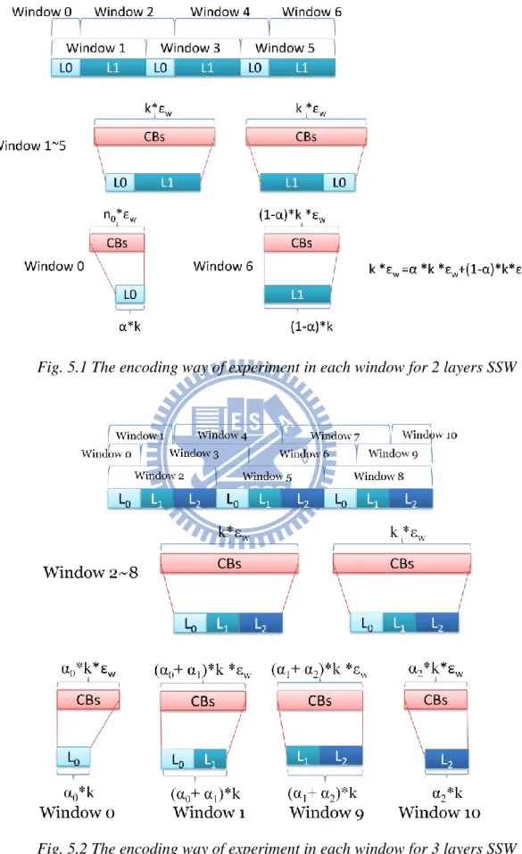
Fig. 5.1 The encoding way of experiment in each window for 2 layers SSW ... 37
Fig. 5.2 The encoding way of experiment in each window for 3 layers SSW ... 37
Fig. 5.3 The deviation in different amount of windows with overhead: 0.04~0.2 k=2000 and the step size=0.02 ... 38
Fig. 5.4 The average prediction error versus total windows graph with k=2000 ... 39
Fig. 5.5 The deviation in different window size ... 40
Fig. 5.6 The encoding structure of SVC streaming ... 42
Fig. 5.7 the relationship between PSNR and displayed frames on different packet loss rate ... 43
Fig. 5.8 The graph of amount of displayed frames of estimation and simulation on different packet loss rate ... 43
Fig. 5.9 The encoding process of [11] ... 45
Fig. 5.10 The encoding process of general LT codes ... 46
vi
Fig. 5.12 Overhead versus displayed frames graph with window size=2033 and total windows =
11 ... 47
Fig. 5.13 Overhead versus PSNR graph with window size=2033 and total windows = 11 ... 48
Fig. 5.14 Overhead versus displayed frames graph with window size=4066 and total windows = 5 ... 48
Fig. 5.15 Overhead versus PSNR graph with window size=4066 and total windows = 5 ... 49
Fig. 5.16 The original bandwidth and the available bandwidth in the experiment ... 50
Fig. 5.17 The amount of Displayed Frames versus time interval graph ... 51
Fig. 5.18 The average PSNR versus time interval graph ... 51
Fig. 5.19 Estimation results and simulations results of SSW with robust soliton distribution, k=2000, total windows=31, α=0.3 and ε=0.04 ... 53
Fig. 5.20 Estimation results and simulations results SSW with robust soliton distribution, k=2000, total windows=31, α=0.3, ε=0.08 ... 53
Fig. A.1 Estimation results and simulations results in section 5.1 with k=2000, total windows=5, α=0.3, (a)ε=0.04, (b) ε=0.06, (c)ε=0.08, (d)ε=0.10, (e)ε=0.12, (f)ε=0.14, (g)ε=0.16, (h)ε=0.18 , and (i)ε=0.20 ... 58
Fig. A.2 Estimation results and simulations results in section 5.1 with k=2000, total windows=11, α=0.3, (a)ε=0.04, (b)ε=0.06, (c)ε=0.08, (d)ε=0.10, (e)ε=0.12, (f)ε=0.14, (g)ε=0.16, (h)ε=0.18 , and (i)ε=0.20 ... 60
Fig. A.3 Estimation results and simulations results in section 5.1 with k=2000, total windows=21, α=0.3, (a)ε=0.04, (b)ε=0.06, (c)ε=0.08, (d)ε=0.10, (e)ε=0.12, (f)ε=0.14, (g)ε=0.16, (h)ε=0.18 , and (i)ε=0.20 ... 62
Fig. A.4 Estimation results and simulations results in section 5.1 with k=2000, total windows=41, α=0.3, (a)ε=0.04, (b)ε=0.06, (c)ε=0.08, (d)ε=0.10, (e)ε=0.12, (f)ε=0.14, (g)ε=0.16, (h)ε=0.18 , and (i)ε=0.20 ... 64
Fig. A.5 Estimation results and simulations results in section 5.1 with k=2000, total windows=101, α=0.3, (a)ε=0.04, (b)ε=0.06, (c)ε=0.08, (d)ε=0.10, (e)ε=0.12, (f)ε=0.14, (g)ε=0.16, (h)ε=0.18 , and (i)ε=0.20 ... 66
Fig. A.6 Estimation results and simulations results in section 5.1 with k=1000, total windows=21, α=0.3, (a)ε=0.04, (b)ε=0.06, (c)ε=0.08, (d)ε=0.10, (e)ε=0.12, (f)ε=0.14, (g)ε=0.16, (h)ε=0.18 , and (i)ε=0.20 ... 68
Fig. A.7 Estimation results and simulations results in section 5.1 with k=4000, total windows=21, α=0.3, (a)ε=0.04, (b)ε=0.06, (c)ε=0.08, (d)ε=0.10, (e)ε=0.12, (f)ε=0.14, (g)ε=0.16, (h)ε=0.18 , and (i)ε=0.2 ... 70
Fig. A.8 Estimation results and simulations results of 3 layers SSW with k=2000, total windows=31,ω0=0.25, α0=0.25, α1=0.25, α2=0.5 (a)ε=0.02, (b)ε=0.05, (c)ε=0.08, (d)ε=0.11, (e)ε=0.14, (f)ε=0.17, (g)ε=0.20 ... 72
Fig. A.9 The deviation of 3 layers SSW with k=2000, total windows=31,ω0=0.25, α0=0.25, α1=0.25, α2=0.5 ... 72
vii
L
L
i
i
s
s
t
t
o
o
f
f
T
T
a
a
b
b
l
l
e
e
s
s
Table I Actual video length and the total required windows with window size = 2000 and
bandwidth = 1000 kbps ... 41 Table II The details of the SVC streaming ... 42 Table III The details of SVC streaming ... 45
1
C
C
h
h
a
a
p
p
t
t
e
e
r
r
1
1
:
:
I
I
n
n
t
t
r
r
o
o
d
d
u
u
c
c
t
t
i
i
o
o
n
n
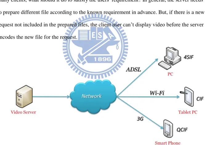
In heterogeneous networks, the client users can connect to Internet by using different devices such as smart phone, tablet PC, or desk-top computer, and those devices can connect to Internet by using different protocols such as xDSL, WiMAX, LTE, 3G,4G, P2P …etc, as shown in the Fig. 1. The different devices mean that the server needs different video
resolution and size to satisfy the users’ requirement and the different protocols mean that the server needs to transmit video at different speed. If there is a server that provides a video to many clients, what should it do to satisfy the users’ requirement? In general, the server needs to prepare different file according to the known requirement in advance. But, if there is a new request not included in the prepared files, the client user can’t display video before the server encodes the new file for the request.
Fig. 1 Heterogeneous networks
In the above example, we can observe that the server needs to encode too many streaming files in order to satisfy different requirement; The loading of server is very huge.
2
Therefore, for reducing server’s loading, the Scalability Video Coding (SVC) [1] is proposed. SVC provides a new way to encode a video that the server only encodes one time, and then there are many layers in the encoded data. Clients can only receive the data that they need, the remain part of data don’t need to be received. By this way, it reduces server’s loading.
When the packet is transmitted, the packet may be lost or be damaged sometimes. In the situation, resending data is one method to solve the problem. Nevertheless in some case like the duty of outer space data transmit or delay sensitive situation, resending data is not allowed. In this situation, somebody tries to recovery the data by using the received data. This method is called “channel coding”.
The Reed Solomon codes (RS codes) [2] is a popular channel coding, but the RS codes has the drawbacks that the encoding and decoding are very complex. For simple encoding and decoding, the” Rateless codes (RS codes)” or “Fountain codes” [3][4][5] method is
proposed. As its name says, this codes is like a fountain: the water is an uninterrupted flow. As we provide some input to the codes, it can generate virtually unlimited outputs. The
characteristic of LT codes is that encoding and decoding are very simple. In fact, it only uses XOR. But it cuts both ways, the LT codes shifts the hard work to define the degree
distribution. The degree distribution plays an important role in LT codes, and it will affect the decoding performance. In [3], M. Luby proposed a good degree distribution, “the robust soliton distribution”. Henceforward the rateless codes becomes a popular research. The methods that use similar idea are proposed such as raptor codes [4] ,Low Density Parity Check(LDPC) codes [6][7], Tornado codes[8] and online codes [9] .
In traditional rateless codes, it provides the equal protection to each data. However, in some case, the data is divided into different degree of importance, so we need to provide
3
“unequal error protection (UEP)” to protect different important data. In [10], UEP is achieved by using the different window sizes. Because the amounts of covered data in different windows are different, the data is covered different times. Thus, the more important data is covered more times, and the data has the more recovery probability. In [11], the UEP is achieved through the way check blocks (CBs) choose their neighbors with different
probability. The parameter kM is used to control the probability that the CBs choose different important MBs .The more important message blocks (MBs) have the higher probability to be chosen as the neighbor of the CBs, so it have more recovery probability. Recently, the
duplicated method is proposed in [12].This method also let the more important message blocks (MBs) have the higher probability to choose the more important MBs, but unlike [11], it duplicates the more important MBs more times, therefore the more important message blocks (MBs) have the higher probability to be chosen as the neighbor of the CBs.
In this paper, we have three contributions. First, we proposed an improved sliding window [13] method, SSW rateless code. This method lets the sliding window provide UEP. Second, we proposed a prediction model that accurately predicts the decoding failure
probability of the MBs in each SVC layer. Third, unlike [14], it uses PSNR as the quality standard, we propose a model that uses the decoding successful probability to predict the total displayed frames. By selecting a best weight that causes the most frames to be displayed, our proposed method provides the best protection and the highest PSNR. Finally, the experiment results show that our method is useful, accurate and more effective than other methods.
This paper is organized as follows. In chapter 2, we describe the tool we will be using. In chapter 3, we describe the related work. In chapter 4, we describe our proposed method. In chapter 5, we will show the experiment results and compare with the other methods. And chapter 6 is the conclusion.
4
C
C
h
h
a
a
p
p
t
t
e
e
r
r
2
2
:
:
B
B
a
a
c
c
k
k
g
g
r
r
o
o
u
u
n
n
d
d
In this chapter, we will introduce the tool that we use in later chapter and the related method that proposed before.
2.1 LT Codes
LT codes [3] is the first practical capacity approaching fountain codes. It is proposed by M.Luby. To begin with, LT codes cuts the input streaming into the same size messages blocks
(MBs). Then, check blocks (CBs) are produced according to the following steps:
1.According to the predefined degree distribution, decide degree for each CB. 2. After getting a degree, each CB selects the same amount of MBs as the neighbors
uniformly.
3. All the data of neighbors of CB are XORed
An example of the LT encoding process is shown in Fig. 2.1.
Fig. 2.1 LT codes encoding process
5
information transmitted to the decoder? In general, there are two ways .The first method is the basic method that transmits all these information directly. The second method is that the encoder and decoder use the same random number generator and the seed that the encoder uses to produce CBs is packaged in the header of the packets. When the decoder receives the seed, CBs can be produced in the same way as the encoder.
After the decoder receives the data from the encoder, decoder uses the belief propagation algorithm to execute the decoding process. The following are the decoding process:
1. Searching for the degree = 1 CB
2. The data of the CB is copied to the only one neighbor.
3. The MB does the XOR with all the neighbors expect the step 1 CB and the degrees of these CBs is decreased by 1.
4. Redo step 1~3 until there is no degree 1 CBs.
So far, we can observe that the LT codes only uses XOR operation to encode and decode, therefore, the operation of the LT codes is much uncomplicated.
Although the LT codes lets the operation to be simple, but it has to pay attention to design the degree distribution. A good degree distribution has the following three features: 1. The less amount of CBs to decode successful.
2. The less amount of CBs of degree.
3. There retain at least one degree =1 CB at any time.
If we use a bad degree distribution, it will cause the number of degree too many or the degree=1 CB is so few that the decoding successful probability of MBs is low. A bad degree distribution example is shown in the Fig. 2.2. In this example, there is only one degree=1 CB. After the decoding process, only one MB can be recovered, and the remaining two MBs can’t be recovered forever. Moreover, too many degrees will cause lots recovery time of MB, but
6
too few degrees will cause the situation where some MBs are not covered. So it is an issue of tradeoff.
Fig. 2.2 Bad degree distribution example
In [3], M. Luby proposed a good degree distribution. In the first, he defined the Ideal Solition Distributionρ (‧):
Assume k is the amount of MBs.
But the problem of the Ideal Solition distribution is that the degree=1 CB does not exist frequently in the decoding process. Therefore, to overcome this problem M. Luby proposed the Robust Solition Distribution μ (‧):
Assume δ as the allowable failure probability of each MB.
7
Finally, after the normalization we can obtain the Robust Solition distribution μ(‧):
μ
Furthermore, LT codes have a cardinal characteristic. Where the more MBs are, the less amount of CBs are required. For this reason, in the more amount MBs environment the LT code can decode more effectively. The relation between MBs and CBs is shown in Fig. 2.3.
8
2.2 Sliding Window
In the section 2.1 description, we could know that the overhead is small when the
amount of the MBs is large. But in video streaming environment, we can’t decode the packets until we receive all the packets, instead, we have to decode when we receive part of packets. Therefore, as shown in the Fig. 2.4, the original data have to be cut into many sections. Then each section is encoded respectively. However when the section is smaller, the LT codes become inefficient.
Fig. 2.4 Data partition
To solve the problem, [13] proposed sliding window (SW) method. Firstly, it decides a window size (same as the section size), and uses LT codes to encode all the data that are covered by the window. Next, it slides the window s MBs size (remove s MBs in the window and join s new MBs) and encode the window again. And it repeats the steps until the SW encodes the last MB. In Fig. 2.5 we can observe the biggest difference between the SW and LT codes is that the SW increases the amount of MBs virtually, hence SW solves the problem that amount of MBs is not enough in certain video streaming environment.
9
Fig. 2.5 Sliding Window encoding process
Then, we are going to analyze the sliding window. Assume there are w MBs and the window size is k MBs. In every step the window slides s MBs. The average of times that each MB is encoded by windows is calculated as the following:
In this sliding way, the amount of windows Ns is
The original data is expanded w’ long.
Next, we calculate the overhead of LT codes.
10
Where n is the amount of CBs and is the overhead.
Now, we can observe that if we want to expend the original data longer, we need to select the smaller s, and vice versa.
Then, we can get the overhead of each virtual MB.
We can get the amount of CBs nw that each window produces:
Finally, we compare the overheads of one window between the LT codes and the SW:
ε ε
We can get the conclusion that each window of SW produces less CBs than the LT codes. Because the windows are overlapped in SW process, the CBs that are received in different window before can help the CBs in this window to decode. Therefore SW let the window to contact with other window. In the end, SW solves the problem that LT codes is ineffective in the less amount of MBs environment.
11
2.3 SVC
Recently, scalability video coding (SVC) is a popular coding method in streaming method, users can arbitrarily choose the packets what they need. Therefore, the server only encodes the video one time and transmits the encoded video to the client users that have different requirements. The server doesn't need to encode the specific video file, so the loading of server is low.
SVC in H.264 has three categories in traditional: temporal scalability, spatial scalability, quality scalability. The examples of those three encoding categories are shown in the Fig 2.6.
Fig. 2.6 Different types of SVC [15]
The three types of SVC will encode the original video file into multi-layer encoded files. When we decode more layers of the video, the displayed video quality is much better. The temporal scalability uses the frame rate to control the size of streaming, when there are more temporal layers, the video is smoother. The spatial scalability uses the video size to control the size of streaming. When we receive more layers, the video displays in bigger size. The quality
12
scalability uses the video quality to control the size of streaming. When we receive more layers, the video is clearer. However, the three types of SVC are not independent of each other, on the contrary, the types of SVC can be combined arbitrarily and decide the amount of layers according to the applications.
Now, we know the types of SVC .Next, we show an example of temporal scalability encodes in Fig. 2.7, and each rectangle stand for a frame in the figure.
Fig. 2.7 SVC 4 Layer encoding example
In here, we can observe that the higher layer frames need to wait the dependent lower layer frames decoding. Before the dependent lower layer frames decode successfully, the higher layer frames can’t decode any frames. Notwithstanding the packets of higher layer frames are received completely, the higher layer frame still can’t be decoded as long as the packets of lower layer frame are lost or damaged. This relationship of the frames is called the dependence of frames. Due to the relationship, frames can be of different importance. That is,
13
the lower layer frames influence more frames, so the lower layer frames are more important; the higher layer frame influence less frames decoding, so the lower layer frames are less important. Due to the different importance of frames, we want to provide the UEP on the sliding window in this paper.
Moreover, because the dependence of frames will cause the order of encode and display discordant, some frames can’t be displayed even though the frames are decoded successfully. The delay due to the encoding structure is called “structure delay”. To avoid the too long structure delay, we will cut the original video into numbers of group of picture (GOP), and each GOP is encoded by the same encoding structure. In some environment like in the real time environment, it is an important factor to consider the structure delay, so the suitable GOP size is important.
14
2.4 And-Or Tree Analysis
The And-Or tree analysis is an analysis method of rateless codes, it is proposed in
[9][16]. The analysis method is very important to analyze the decoding failure probability of
LT codes.
In order to analyze the decoding failure probability, we first cut the original data into numbers of same size message blocks (MBs), these MBs transfer to OR-nodes (Because a MB can be recovered as long as there exists one neighbor that can recover it). The check blocks (CBs) transfer to AND-nodes (Because a CB can not recovery a MB as long as there is only one neighbor that is not recovered yet)
When the AND-node and OR-node is neighbor, the nodes connect with an edge. And then we randomly choose one OR-node as the root of the tree; meanwhile, we randomly choose one edge that connects to the root OR-node and delete it. Now we pull the node up and produce an 2i height AND-OR tree GTi .The tree consists of OR-node at level 0,2,4,…,2i
and the tree consists of AND-node at level 1,3,5,…,2i-1. At level i leaf, the AND-node
randomly pass 0 or 1 to the level i OR-node. When the OR-node is at level i leaf, the OR-node is certain that pass 1 to the level i+1 AND-node. In other cases, the level i AND-node will pass 1 to the level i OR-node when all of children of the AND-node pass 1 to it. The level i OR-node will pass 1 to the level i+1 AND-node when there exists one child pass 1 to the OR-node. And the remaining cases, the AND-node and OR-node pass 0 to its parent. We do this process from the leaf to the root, and we finally obtain the probability yi that the value of
root of the tree GTi is 0.
15
Assume the high of the tree is l and the root of the tree is 0 with the probability yl
α
α α
where α i is the probability that an OR-node has i children and A is the maximal amount of
total children of an OR-node.Similarly, β i is the probability that an AND-node has i children
and B is the maximal amount of total children of an OR-node.
In chapter 4, we will use the And-Or tree lemma to estimate the decoding failure probability of different layer MBs.
16
C
C
h
h
a
a
p
p
t
t
e
e
r
r
3
3
:
:
R
R
e
e
l
l
a
a
t
t
e
e
d
d
W
W
o
o
r
r
k
k
s
s
In this chapter, we describe the relative UEP methods that proposed before. 3.1 Expanding Window Fountain
In [10], this paper proposed an UEP method “Expanding Window Fountain (EWF)”. Assume there are k MBs, these MBs partition into N different important classes and each class has nj MBs ( n0+n1+n2+n3+….+nN-1= k ). In these classes, the class is more important when class index is less, so the n0 is the most important class and the nN-1 is the least important class. Then, there are N windows and the j th window have MBs. When generating the check blocks(CBs) , each CB randomly chooses the window according to the window selection distribution , where is the probability that i th window is chosen. Then, each window has its own degree distribution
, where is produced by the the robust solition distribution when . The following is the encoding process:
1. Choosing one window j according to Γ .
2. According to the Ω , one degree is decided for each CB.
3. After getting a degree, each CB selects the same amount of MBs as the neighbors uniformly.
4. All the data of neighbors are XORed to produce the CB. The decoding process is same as the LT codes.
17
Fig. 3.1 Encoding process of EWF
Finally, the EWF realizes the UEP according to the overlapped window , the MBs in n0 is covered the most times, so most CBs have the data .Therefore the MBs in n0 has the most protection.
For the video streaming applications, the original data needs to be cut into a number of sections. Each section is smaller than the size of the original data and the windows of EWF are smaller than or equal to the section. Because of the property of LT codes, the decoding performance will suffer when the window length becomes smaller. Therefore, EWF is not quite unsuitable for video streaming.
18
3.2 The UEP Method of “Rateless Codes
With Unequal Error Protection Property”
[11]
In [11], it proposed an UEP method for two layers MBs: more important bits(MIB) and less important bits (LIB). It provides the UEP to ensure the MIB that has the higher decoding successful probability than the LIB. The parameters kM and kL mean the protection levels for the MIB and LIB. Assume the data amount is n, the amount of data in MIB is α and the amount of data in LIB is α . The method uses the
probability and ( α
α and ) to decide the probability that each data in MIB or LIB is chosen as the neighbor of CBs.
And it uses the degree distribution (1) that describe in Raptor codes [4]
(1)
The following is the encoding process:
1. According to the (1), decide the degree for each CB.
2. After getting a degree, each CB selects the same amount of MBs according to the probability p0 and p1.
3. All the data of neighbors of CB are XORed to produce a CB The decoding process is the same as the LT codes.
This paper also proposed a prediction model that estimates the decoding failure probability of MIB and LIB according to AND-OR tree analysis [9][16]. Assume the average CB degree is μ and there are CBs. The decoding failure probability of MIB and
19
LIB are and when the tree height is 2l .The prediction model is shown in (2)(3):
μ α α (2)
μ α α (3)
(4)
This method will be compared with our proposed method in section 5.3.
But, as shown in Fig. 3.2, the accuracy of the prediction model is not quite well. The prediction error is between 15% and 45%. Where the prediction error is defined as .
20
Fig. 3.2 The deviation of [11] with overhead: 0.04~0.2 and the step size=0.02,n=2000 ,kM=1~3 and total section=11
3.3 The UEP Method of “Unequal Error
Protection Using Fountain Codes with
Applications to Video Communication”
[12]In [12], this paper proposed a method that uses duplication idea. Assume the MBs are partitioned into N different important classes. Each class has nj MBs and the total MBs is
n=n0+n1+…+nN-1. In the beginning, the idea is like the sliding window [13], it tries to virtually expand the window size and solve the problem that the performance of LT codes is not good when the input MBs are not enough. Hence, this method uses the expanding factor
EF to duplicate the original data EF times, so the amount of original MBs replace n by EF*n.
Then ,when the amount of MBs is become larger ,the degree distribution change according to in the robust solition distribution. Besides, when the CBs choose one index of MBs j, and the index j is replaced by j mod n. Next, in order to provide the UEP, this method use the repeat factor RFi , i=0,..,N-1 to duplicate the class i MBs by RFi times. So, there are
21
MBs of different class are chose as the neighbor of CB. Therefore, when the CB chooses one index of MBs l, and it have to replace the l according to (5).
(5)
The example of encoding process is shown in Fig. 3.3:
Fig. 3.3 Example of encoding process of [12] with n0=2, n1=1,
RF0=2, RF1=1 and EF=2
Since the work in [12] does not provide the corresponding prediction model, we don’t know how to decide the best EF and RFi.
22
C
C
h
h
a
a
p
p
t
t
e
e
r
r
4
4
:
:
P
P
r
r
o
o
p
p
o
o
s
s
e
e
d
d
M
M
e
e
t
t
h
h
o
o
d
d
In this chapter, we will introduce our proposed method first. By using the method, we will protect different important data at different protection level in section 4.2. And then, we will use the And-Or tree analysis to analyze our proposed method. We propose a model that can estimate the status of MBs after the sliding window decoding process. Finally we propose a prediction model that predicts the amount of frames that can be displayed when we use our proposed method on SVC streaming.
4.1Proposed Synchronized Sliding
Window Rateless Codes
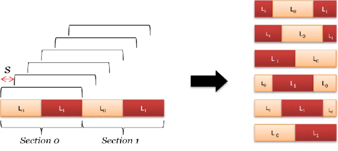
In traditional sliding window, there are some obstructs when it tries to provide UEP. The first problem is that there are windows changes when the window slides each time. For example in Fig. 4.1, the MBs in first window consist of layer 0 MBs and layer 1 MBs in section 0.But after the window slides s MBs, the second window consists of part of encoded layer 0 MBs in section 0, encoded layer 1 MBs in section 0, and part of layer 0 MBs in section 1. In one window, some MBs have been encoded and some have not. It is very difficult to protect and analyze in this situation. The second problem is how long does the window slide in each time. In section 2.2, we know that the distance of one sliding influence the encoding times of each MB. To decide s is also an issue.
23
Fig. 4.1 The content of each window in sliding window
Therefore, we modify the traditional sliding window in order to not only avoid the above problems but also let the sliding window simpler when it is used in UEP.
Firstly, we classify the data as N level according to their importance, and the most important data is classified as the L0 data with the weight ω0, the second important data is classified as
the L1 data with the weight ω1,…, and the least important is classified as the LN-1 data with
the weight ωN-1. Then, as what Fig. 4.2 shows, we cut the MBs into each section according
to the order L0 ,L1,…, LN-1,and the amount of different level MBs can be different.
24
In the following, we will describe the encoding process of SSW. The first step, the first window encode the MBs of section 0, but the encoding process has some difference between the traditional LT codes, that is, when one CB chooses their neighbors, we use the probability
pj ,j=0,…,N-1,to decide the probability that an layer j MB is chosen as the neighbors of the
CB.
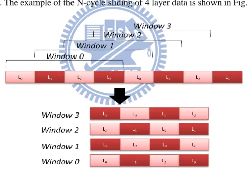
After the first window produce CBs, we slides the window, but in our proposed method, instead of sliding in fixed step, we slide the window by the amount of L0 MBs at the first time, we slide the window by the amount of L1 MBs at the second time, and so on. After the N time sliding, the window slides the window by the amount of L0 MBs again. Therefore, the sliding is an N-cycle. The example of the N-cycle sliding of 4 layer data is shown in Fig. 4.3.
Fig. 4.3 Example of N-Cycle sliding of SSW on 4 layer input data and the content of each window
We can observe that there does not exist the data that some have been encoded and some have not in any layer .By using the way of sliding, the content of the window is more simple and become easier to protect and analyze.
25
4.2 Prediction Model
In this section, we will do the And-Or tree analysis [9][16] for SSW. First, we transmit the message block(MBs) into the OR-node, and we transmit the check block(CBs) into the AND-node. In each window, it contains k OR-nodes. And each window will produce γw*k AND-nodes. Then, we set the weight ωj for Layer j OR-node . Similar to the way of And-Or
tree analysis described in section 2.4, we build the And-Or tree GTi,j. GTi,j mean that the
height of the And-Or tree is 2i and the root is a layer j OR-node. Our goal is to obtain the probability pi,j that the root of the tree is 0 after the And-Or tree analysis.
4.2.1 The probability that a level i AND-node will pass
the 0 to the level i OR-node
Firstly, we are going to calculate the probability qi that a level i AND-node will pass 0 to
the level i OR-node. We define the amount of the edges that connect a level i AND-node and level i-1 OR-nodes that is dj. Fig. 4.4 is the example of the connection of an AND-node . We can obtain the qi when we know the amount of degrees that connect to each layer OR-node in level i, as show in (6):
Fig. 4.4 The way of connection of a AND-node in AND-OR tree
26
(6)
The amount of degrees that an level i AND-node connect to layer j OR-node in level i-1 is dj ,
j=0,…,N-1 . In the latter part of (6), it represents the situation that a level i AND-node will pass 1 to the level i OR-node. This situation will happen only when all of the level i-1 OR-nodes pass 1 to the level i AND-node. And (6) removes the situation and obtains the probability that a level i AND-node passes the 0 to the level i OR-node. By using the
predefined degree distribution (x) and d is the probability that the degree of a CB is d. In (7), we can obtain the average degree of each CB μ.
μ (7)
In (8), We also calculate the probability Ad that an edge connects to an degree d AND-node
μ (8)
We can finally obtain the qi:
(9)
In first summation, it decides the different degree d of the AND-node (d has removed the edge that connect to the level i OR-node) and then it multiplies the occurrence probability Ad+1. The second summation decides dj, and then it multiplies the occurrence probability that is calculated by Wallenus’s distribution. Therefore, we can obtain each probability by (1) in different degree distribution and obtain qi finally.
27
(10)
The q0 is the probability that the AND-OR tree leaf passes 0. Because the leafs have no children, so
the situation that the leaf AND-node passes 1 to the OR-node only occurs when the degree of leaf AND-node is 1. Hence we obtain q0 as long as we reduce the probability 1.
4.2.2 The probability that a level i OR-node will pass 0
to a level i+1 AND-node
In order to obtain the probability pi,j that a level i OR-node will pass 1 to a level i+1
AND-node, we have to calculate the probability pj that an edge connects to a certain layer j
OR-node and as shown in Fig. 4.5. In layer j ,each OR-node set the weight ωj. Then, the
probability that each MB is chosen as the neighbor of one CB is shown in (11), and the probability is equal to pj.
ω
ω ω (11)
Fig. 4.5 Pj
28
We calculate the probability λ d,j that a layer j OR-node has d degrees:
μ μ
(12)
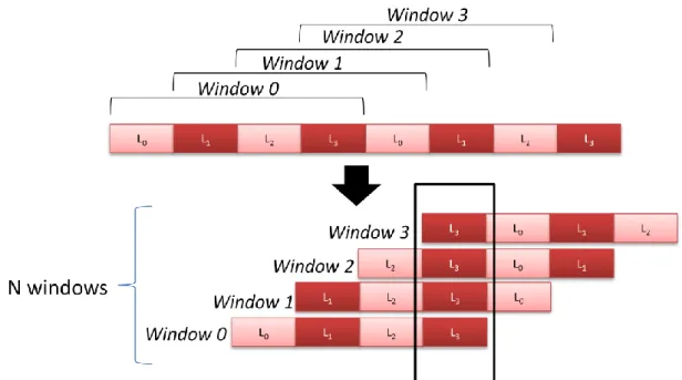
In (12), the summation distributes the degree to each window, and it mean that the OR-node get mj degrees from j th window (Each MB is covered by N windows). And because the
numbers of MBs in each layer are the same in each window, the probability pj is the same for all N windows. Hence, the probability that an MB get mx degrees from window x is
μ μ
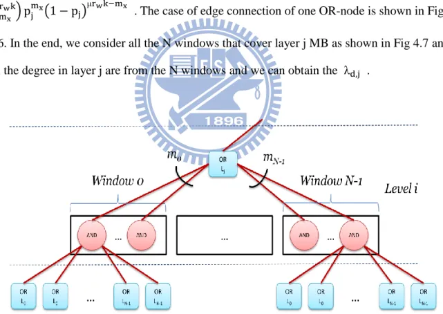
. The case of edge connection of one OR-node is shown in Fig. 4.6. In the end, we consider all the N windows that cover layer j MB as shown in Fig 4.7 and all the degree in layer j are from the N windows and we can obtain the .
29
Fig. 4.7 The example of layer 3 MBs are covered by 4 windows when N=4
By using , we can obtain the probability Rd,j that an edge which connects to a layer j
OR-node has degree d:
μ μ μ (13) In (13), assume there are nj layer j MBs in one window. The denominator means that the sum of the edges that connect to a layer j OR-node from all the N windows, and the numerator means that the sum of the edges that belong to the lay j MBs with degree d. The probability for a level i OR-node to pass 1 to a level i+1 AND-node is:
μ
(14)
30
4.2.3 To simplify
μ μ μ μ μ μ μ μ (15)
According to Binomial theorem μ μ μ μ (16) μ μ μ μ μ μ (18)
31 μ μ μ μ μ μ μ According to Taylor series expansion
μ μ
32
4.3 Selecting Best Weight
In order to own the best video quality, in general, the PSNR can be used to estimate the difference between the original video and the processed video. But, if some frames are damage or lost, those damaged or lost frames have to be concealed by the closest frame. In this case, it is very difficult to estimate the PSNR because the closest frame can be anywhere and the distance of the closest frame will affect the relevance of content. If the distance is close, the content is similar and the PSNR is better. Oppositely, if the distance is far, the content is not similar and the PSNR is low. Therefore, we observe that the PSNR is higher when there are more frames is received. The different amount of frames example is shown in the Fig. 4.8. In this example, the video 3 has the best video quality because the average distance of the copy fame is shorter than video 1 and video 2. Even in the extreme case that all the frames are received, more frame case also has the shortest distance, so it has the best video quality.
Fig. 4.8 Displaying the different amount of frames video
33
PSNR. In our goal, we estimate which weight can produce the most displayed frames. Firstly, we observe the expected value in (20) and the dependence of SVC encoding structure of Fig. 4.9. The dependence of frames are shown in Fig. 4.10, and the edge connect with two frames that have the dependence relations.
Fig. 4.9 The encoding Structure of SVC streaming
34 (20)
We can obtain the simplified equation (21) from (20). Assume P(Layer i) is the probability that all of the packets of a layer i frame are received successfully and it can be obtained from the pi,j in(14). For example, if a layer j frame needs u packets to transmit, and the
P(Layer i)= Pi,ju .Assume the dep(Layer i) is the amount of dependent frames in the Layer i+1. In section 5.2, we will verify if the model is feasible later.
(21)
At this time, we have the model to estimate the weight which can produce the best quality video and we will use this model on SVC streaming environment in next chapter.
35
C
C
h
h
a
a
p
p
t
t
e
e
r
r
5
5
:
:
T
T
h
h
e
e
E
E
x
x
p
p
e
e
r
r
i
i
m
m
e
e
n
n
t
t
R
R
e
e
s
s
u
u
l
l
t
t
s
s
In this chapter, we will check if our proposed prediction model is accurate or not;meanwhile, we will also find the suitable environment for the prediction model. Then, we will verify the feasibility of the prediction model in section 4.3 about the amount of displayed frames to select the best weight. After we verify the prediction model for selecting the best weight, we not only use our proposed method with SVC streaming but also compare with the other methods. Finally, we use the proposed method on variable bandwidth environment.
5.1 Accuracy Analysis for SSW Rateless
Codes Model
In this section, we will observe whether the simulation estimation results near the simulation results or not. In other words, we observe whether our prediction model can be used to estimate our proposed method.
The following is our experiment environment for 2 layers SSW: Total layers of sliding window: 2
Window size k: 1000, 2000,4000
The amount of window: 5, 11, 21, 41,101 α = : 0.3
w0: 0.05~0.95 (step size:0.05) Repeat time of each weight: 100 ε:0.04~0.2 (step size:0.02)
36
The following is our experiment environment for 3 layers SSW: Total layers of sliding window: 3
Window size k: 2000 The amount of window: 31
α 0= : 0.25 , α 1= : 0.25, α 2= : 0.5 w0:0.25, w1: 0.05~0.7 (step size:0.05)
Repeat time of each weight: 100 ε:0.02~0.2 (step size:0.03)
We use the degree distribution of Raptor codes [4] in the following experiments:
(22)
To deal with first and last windows, the 2 layers SSW with 5 windows example is shown in Fig. 5.1. In this example, window 0 and window 6 are included in the encoding process and the sum of their MBs is equal to one window. The Fig. 5.2 is the 3 layers SSW with 8
windows example. In this example, window 0, 1, 9, and window 10 are included in the encoding process. After adding these extra windows, we have to reduce CBs that each window produces, so that the overhead keeps the same.
37
Fig. 5.1 The encoding way of experiment in each window for 2 layers SSW
38
After setting the experiment environment, we observe the accuracy of the proposed method in different amount of windows (5, 11, 21, 41, and 101).The 2 layers experiment results are shown in Fig A.1-A.5 in appendix A and Fig. 5.3-5.4, and 3 layers SSW with 31 windows experiment results are shown in Fig A.7-A.9.
Where the prediction error is defined as
ω
Fig. 5.3 The deviation in different amount of windows with overhead: 0.04~0.2 k=2000 and the step size=0.02
39
Fig. 5.4 The average prediction error versus total windows graph with k=2000
From these results, we can observe that prediction model is inaccurate in some scope of weights when the overheads are less. Besides, the model is accurate after the overhead
exceeds a threshold and the threshold becomes lower when the amount of windows increases. It is possible that the influence of the first and last window become smaller when the amount of windows becomes more.
Then, we observe that the influence of the window size on prediction. The experiment results are shown in Fig. A.3, A.6 and A.7 in appendix A and Fig. 5.5:
40
Fig. 5.5 The deviation in different window size
In Fig. 5.5 we can note that prediction model is inaccurate when the window size is small in some scope of weights. Besides, the threshold of overhead of prediction model is smaller when we use the bigger window size.
According to the above experiment results, we conclude the prediction model is accurate when the amounts of the windows are more or the windows size is bigger.
Moreover, assume the bandwidth is 1000 kbps, packet size 1500 Bytes and the window size is 2000 packets. The actual video length and the window they require in are shown in Table I. It shows that our proposed method is useful for music video, soap operator and movie.
41
Video Length Total Windows
Music Video 3mins - 6mins 15 - 31
Soap Operator 25mins - 60mins 127 - 307
Movie 90mins - 120mins 461 - 615
Table I Actual video length and the total required windows with window size = 2000 and bandwidth = 1000 kbps
5.2 Confirm Relationship of PSNR and
Total Displayed Frames
In this section, we will explain why our prediction model in section 4.3 estimates the displayed frames instead of PSNR. The following is the experiment environment:
Packet loss rate: 0.01~0.1(step size=0.01) Packet size : 1500 Bytes
Repeat times of each packet loss rate : 100 5 layer of temporal scalability
The decoder certainly received SPS(Sequence Parameter Set) ,PPS(Picture Parameter Set) ,and Frame 0. The encoding structure of SVC streaming is shown the Fig. 5.6 and Table II is the details of SVC input file.
42
Fig. 5.6 The encoding structure of SVC streaming
SOCCER_3 52x288_30_ orig_02.yuv bit rate (kbits/sec) QP The average packets of one frame The total frame of one GOP GOP size T0 382.01 18 16.78 1 16 T1 506.57 22 6.28 1 Total GOP T2 672.66 23 4.30 2 19 T3 880.28 24 2.81 4 Total frame T4 1093.70 26 1.69 8 289 IDR 16
Table II The details of the SVC streaming
In this experiment, we will use different packet loss rates to decide whether each frame is received or not. And a frame can be displayed only when all of the packets are received. We measure the PSNR and the amount of the displayed frames in each packet loss rate. In Fig. 5.7, we can observe that the PSNR is higher when the number of displayed frames increases. Therefore, it is available to use the amount of frames to estimate which weight produce the best quality video. In Fig. 5.8, the estimation result is close to the simulation result, so we will
43
use this model in next section.
Fig. 5.7 the relationship between PSNR and displayed frames on different packet loss rate
Fig. 5.8 The graph of amount of displayed frames of estimation and simulation on different packet loss rate
44
5.3 SSW on SVC Streaming Environment
In this section, we will use the proposed sliding window method on the SVC streaming; meanwhile, we will compare the result with the other methods. The following is experiment environment:
We fill up 0 when the data length of encoded frame in SVC, so each frames in the same temporal layer use the same amount of packets.
SVC layer 0 ,and 1 belong to Sliding Window layer 0 SVC layer 2, 3, and 4 belong to Sliding Window layer 1 Window size k=2033,4066 MBs= 19,38 GOPs
w0: 0.0~1.0 (step size:0.05) Total windows = 5,11 ε = 0~0.2 (step size 0.01) α = 0.3084
Packet size : 1500 Bytes
Repeat times of each point: 100
The decoder certainly received SPS(Sequence Parameter Set) ,PPS(Picture Parameter Set) ,and Frame 0.
45
Table III is the details of SVC input file: SOCCER_ 352x288_3 0_orig_02.y uv bit rate (kbits/sec) QP The number of packets of one frame The total frame of one GOP Total packets of each layer GOP size T0 364.49 18 23 1 23 16 T1 494.31 22 10 1 10 Total GOP T2 660.14 23 9 2 18 115 T3 872.54 24 8 4 32 Total frame T4 1086.53 26 3 8 24 1825 107 IDR 16 Table III The details of SVC streaming
The following are the three competitors: 1. The UEP method [11]:
This method is the same as the description in section 3.1. It doesn’t use the overlapped window and it provides UEP according to the kM. We will use the prediction formula (2)(3) in section 3.1 with the prediction model described in section 4.3 to choose the kM that causes the biggest PSNR. The kM is searched from 1 to 3.24. The encoding process is shown in Fig 5.9.
46
2. General LT codes:
The general LT codes encodes each section without overlapped window and UEP. And it uses the degree distribution (22). The encoding process is shown in Fig 5.10.
Fig. 5.10 The encoding process of general LT codes 3. General LT codes with each layer MBs encoded respectively
The competitor 3 is the same as the competitor 2 without overlapped window and UEP. But its layer 0 MBs and layer 1 MBs are encoded respectively, so the neighbor of CBs either layer 0 MBs or layer 1 MBs. And it also uses the degree distribution (22). The encoding process is shown in Fig 5.11.
Fig. 5.11 The encoding process of general LT codes with each layer MBs encode respectively
47
The experiment results are shown in the Fig. 5.12 - Fig. 5.15. The decoding performance of SSW is better than the other methods, especially in low overhead environment. It is
because the overlapped window connected the relation between each CB in different window. When CBs have the relationship, all the received CBs before can help the decoding process in later window. Furthermore, the estimation is inaccurate in the low overhead because the overhead does not exceed the threshold. The method that layer 0 MBs and layer 1MBs encoded respectively use the less Mbs to encode each layer MBs, so it has the worse
performance than the the method that encode each layer MBs together. The experiment results show that our estimation is more accurate than the method [11].
Fig. 5.12 Overhead versus displayed frames graph with window size=2033 and total
48
Fig. 5.13 Overhead versus PSNR graph with window size=2033 and total windows = 11
Fig. 5.14 Overhead versus displayed frames graph with window size=4066 and total
49
Fig. 5.15 Overhead versus PSNR graph with window size=4066 and total windows = 5
5.4 SSW on SVC Streaming with
Variable Bandwidth Environment
In this section, we will use our proposed method on SVC streaming with bandwidth environment. We will verify the accuracy of the prediction model. The following is the experiment environment:
SVC layer 0 and 1 belong to Sliding Window layer 0 SVC layer 2, 3,and 4 belong to Sliding Window layer 1 Window size k=2033 MBs= 19 GOPs
w0: 0.0~1.0 (step size:0.05) Total windows = 11
α = 0.3084
Packet size : 1500 Bytes
50
The input SVC video is the same as Table III in section5.3. And we also use the competitor 1 in section 5.3 to compare with our proposed method.
The original bandwidth is shown in Fig. 5.16 and we will use the smallest maximum available bandwidth in each time interval of window. The blue line in Fig. 5.16 is the
bandwidth that we use in the experiment. Because our method has the overlapped window so each window only uses half of bandwidth.
Fig. 5.16 The original bandwidth and the available bandwidth in the experiment
The experiment results are shown in Fig.5.17 and Fig. 5.18. The results show that our prediction model is useful when the bandwidth is variable and the competitor is not well because the overhead is not enough.
51
Fig. 5.17 The amount of Displayed Frames versus time interval graph
52
5.5 Performance of the Proposed Model
with Robust Soliton Distribution
In this section, we will observe the performance of SSW with the robust soliton distribution.
The following is our experiment environment: Total layers of sliding window: 2
Window size k: 2000 The amount of window: 21 w0: 0.05~0.95 (step size:0.05) Repeat time of each weight: 100 α = 0.3
ε:0.04,0.08
c:0.01 & δ :0.05 (for robust soliton distribution)
Same as the section 5.1, we also use the two extra windows to deal with the first and the last windows. After setting the experiment environment, we observe the accuracy of the proposed prediction model. The experiment results are shown in Fig 5.19 and Fig 5.20. In Fig 5.19 and Fig 5.20, because the figure can’t be shown when the decoding failure probability is 0, so we set the decoding failure probability as 1E-10 when it is 0.
53
Fig. 5.19 Estimation results and simulations results of SSW with robust soliton distribution, k=2000, total windows=31, α=0.3 and ε=0.04
Fig. 5.20 Estimation results and simulations results SSW with robust soliton distribution, k=2000, total windows=31, α=0.3, ε=0.08
54
C
C
h
h
a
a
p
p
t
t
e
e
r
r
6
6
:
:
C
C
o
o
n
n
c
c
l
l
u
u
s
s
i
i
o
o
n
n
In this paper, we proposed a new sliding window method, Synchronized Sliding Window (SSW) Rateless Coding for layered data or scalable video data, which can provide the UEP on SVC streaming environment. In SSW, we change the way of sliding in sliding window to simplify the component of each window and the analysis process. To realize the UEP, we set weights for each layer MBs. According to the weights, the CBs choose their neighbors in the way that the MBs can be protected at different levels. Then, we analyze our proposed method by AND-OR tree analysis and we successfully proposed a prediction model. When we have this model, we can estimate the decoding failure probability of the MBs of each layer and decide the weights for any environment or requirement. By using the prediction model shown above, we proposed the other prediction model that estimates the amount of displayed frames, and we do the experiments that show the prediction model is feasible. Finally, we use the model to provide the best video quality in SVC streaming.
The experiment results show that our prediction model is excellent in terms of estimation accuracy. On SVC streaming environment, the experiment results show that our proposed method use the least overhead and provide the best quality in the meanwhile. In the variable bandwidth environment, our prediction approach also works well when compared with other methods in the literature.
55
R
R
e
e
f
f
e
e
r
r
e
e
n
n
c
c
e
e
s
s
[
[11]] H. Schwarz, D. Marpe, and T. Wiegand, “Overview of the Scalable Video Coding Extension of the H.264/AVC Standard,” IEEE Transactions on Circuits and Systems for Video
Technology, 17, no. 9, pp. 1103-1120, September 2007.
[
[22]] I. S. Reed and G. Solomon, “Polynomial Codes Over Certain Finite Fields,” Journal of the
Society for Industrial and Applied Mathematics, 8, no. 2, pp. 300-304 ,June 1960.
[
[33]] M. Luby, “LT Codes,” The 43rd Annual IEEE Symposium on Foundations of Computer
Science, 2002. Proceedings, pp. 271- 280, 2002.
[
[44]] A. Shokrollahi, “Raptor Codes,” IEEE Transactions on Information Theory, vol.52, pp.
2551-2567, June 2006.
[
[55]] M. Mitzenmacher, “Digital Fountains: A Survey and Look Forward,” IEEE Information
Theory Workshop, 2004, pp. 271- 276 , 2004.
[
[66]] R. Gallager, “Low-Density Parity-Check Codes,” IRE Transactions on Information Theory 8,
no. 1, pp. 21-28 , January 1962.
[
[77]] J. S Plank and M.G. Thomason “On the Practical Use of LDPC Erasure Codes for Distributed Storage Applications,” 2003.
[
[88]] M. G. Luby, M. Mitzenmacher, M. A. Shokrollahi and D. A. Spielman, “Efficient Erasure Correcting Codes,” IEEE Transactions on Information Theory, vol. 47, pp. 569–584, February
2001.
[
[99]] P. Maymounkov, “Online Codes,” NYU Technical Report TR2003-883, 2002. [
[1100]] D. Sejdinovic, D. Vukobratovic, A. Doufexi, V. Senk and R. Piechocki, “Expanding Window Fountain Codes For Unequal Error Protection,” IEEE Transactions on Communications, 57,
![Fig. 2.6 Different types of SVC [15]](https://thumb-ap.123doks.com/thumbv2/9libinfo/8612122.190798/20.892.203.722.532.858/fig-different-types-of-svc.webp)
![Fig. 3.2 The deviation of [11] with overhead: 0.04~0.2 and the step size=0.02,n=2000 ,kM=1~3 and total section=11](https://thumb-ap.123doks.com/thumbv2/9libinfo/8612122.190798/29.892.305.655.104.414/fig-deviation-overhead-step-size-km-total-section.webp)
![Fig. 3.3 Example of encoding process of [12] with n 0 =2, n 1 =1, RF 0 =2, RF 1 =1 and EF=2](https://thumb-ap.123doks.com/thumbv2/9libinfo/8612122.190798/30.892.131.811.231.394/fig-example-encoding-process-n-rf-rf-ef.webp)