A STUDY ON CADASTRAL COORDINATE TRANSFORMATION USING ARTIFICIAL NEURAL NETWORK
Lao-Sheng Lin
Associate Professor, Department of Land Economics National Chengchi University
64, Section 2, Chihnan Road, Taipei 116, Taiwan Email: [email protected]
Yi-Jing Wang
Graduate of Department of Land Economics National Chengchi University
64, Section 2, Chihnan Road, Taipei 116, Taiwan
KEY WORDS: Artificial Neural Network (ANN), Cadastral Coordinate, Coordinate Transformation, TWD67 (Taiwan Datum 1967), TWD97 (Taiwan Datum 1997)
ABSTRACT: Currently, there are two cadastral coordinate systems used in Taiwan. They are TWD97 (Taiwan Datum 1997) and TWD67 (Taiwan Datum 1967) cadastral coordinate systems respectively. Frequently it is necessary to transform from one coordinate system to another. One of the widely used methods is Least-Squares with affine transformations. The artificial neural network (ANN) provides a new technology for cadastral coordinate transformation. The popularity of this methodology is rapidly growing. The greatest advantage of ANN is that it can be used very successfully with a huge quantity of data and free-model estimation that traditional transformation methods cannot be applied. In this paper, coordinate transformations between TWD67 and TWD97 with artificial neural network (ANN) and Least-Squares with affine transformations were examined. Three data sets with varied sizes from the Taiwan region are used to test the proposed algorithms. The test results show that the coordinate transformation accuracies using the ANN method are better than those of using other methods, such as, Least-Squares with affine transformations. The proposed algorithms and the detailed test results will be presented in this paper.
1. INTRODUCTION
Currently, there are two cadastral coordinate systems used in Taiwan. They are Taiwan Datum 1997 (TWD97) and Taiwan Datum 1967 (TWD67) cadastral coordinate systems respectively. Frequently it is necessary to transform from one coordinate system to another. One of the widely used methods is Least-Squares with affine transformations.
On the other hand, the artificial neural network (ANN) provides a new technology for cadastral coordinate transformation. The popularity of this methodology is rapidly growing. The greatest advantage of ANN is that it can be used very successfully with a huge quantity of data and free-model estimation that traditional transformation methods cannot be applied.
In this paper, coordinate transformations between TWD67 and TWD97 using artificial neural network (ANN) were proposed and examined by the authors. Three data sets with varied sizes from the Taiwan region are used to test the proposed algorithms. The test results show that the coordinate transformation accuracies using the ANN method are better than those of using other methods, such as, Least-Squares with affine transformations. The proposed algorithms and the detailed test results are presented in this paper.
2. ARTIFICIAL NEURAL NETWORK
Artificial neural networks (ANNs) are composed of simple elements operating in parallel. These elements are inspired by biological nervous systems. As in nature, the network function is determined largely by the connections between elements. One can train a neural network to perform a particular function by adjusting the values of the connections (weights) between elements. Normally, neural networks are adjusted, or trained, so that a particular input leads to a specific target output. The network is adjusted, based on a comparison of the output and the target, until the network output matches the target. Typically many such input/target pairs are used, in this supervised learning, to train a network (Demuth and Beale, 2002).
Neural networks have been trained to perform complex functions in various fields of application including pattern recognition, identification, classification, speech, vision, and control systems. Back-propagation (BP) was created by generalizing the Widrow-Hoff learning rule to multiple-layer networks and nonlinear differentiable transfer functions. Input vectors and the corresponding target vectors are used to train a network until it can approximate a function, associate input vectors with specific output vectors, or classify input vectors in an appropriate way as defined by you. Networks with biases, a sigmoid layer, and a linear output layer are capable of approximating any function with a finite number of discontinuities (ibiz.).
3. CADASTRAL COORDINATE TRANSFORMATION USING LEAST SQUARES ADJUSTMENT METHODS
Rectangular X and Y coordinates of any point give its position with respect to an arbitrarily selected pair of mutually perpendicular reference axes. The X coordinate is the perpendicular distance, in feet or meters, from the point to the Y axis; the Y coordinate is the perpendicular distance to the X axis. In cadastral coordinate system, the Y axis points north-south, with north the positive Y direction. And, the X axis runs east-west, with positive X being east (Wolf and Ghilani, 2002). Since the cadastral coordinates are the outputs of a selected map projection method, such as Transverse Mercator (TM). Besides, the cadastral coordinates are highly depended on the selected geodetic datum. For example, there are 2 different types of geodetic datum used in Taiwan region, i.e. TWD67 and TWD97 respectively. For any point in Taiwan region, it has TWD67 and TWD97 cadastral coordinate systems. Hence, it needs some methods to transform the TWD67 coordinate system to the TWD97 coordinate system or vice versa. The points with known TWD67 coordinates, i.e.,
(
X67,Y67)
, and TWD97 coordinates, i.e.,(
X97,Y97)
, will be defined as reference points. Suppose there are n reference points in a region ofinterest. One can uses these known TWD67 and TWD97 coordinates from those reference points to estimate the coordinate transformation parameters, such as rotation, scaling, and translation, etc., applying some kinds of coordinate transformation algorithms, e.g. two-dimensional conformal coordinate transformation or artificial neural network.
Taking the two-dimensional conformal coordinate transformation (the so-called 4-parameter coordinate transformation) as an example, suppose there are n reference points with known TWD67 and TWD97 coordinates in one area. The relationship between TWD67 coordinates and TWD97 coordinates can be expressed by equation (1).
d aX bY X c bX aY Y + − = + + = 67 67 97 67 67 97 (1)
where
(
X67,Y67)
and(
X97,Y97)
are TWD67 coordinates and TWD97 coordinates respectively, a, b, c, and d are the 4 coordinate transformation parameters. The coordinate transformation parameters can be estimated by the least squares adjustment method. For a new point in the same region, with known TWD67 coordinates,(
X67,Y67)
, its TWD97 coordinates,(
X97,Y97)
, can be determined by equation (1) if these coordinate transformation parameters, i.e. a, b, c, and d, are known.Usually, there is another method used to transform coordinates, i.e., 6-parameter coordinate transformation. The following equations express the relationship between TWD67 and TWD97 coordinates: f eX dY X c bX aY Y + + = + + = 67 67 97 67 67 97 (2)
where a, b, c, d, e, and f are the 6 coordinate transformation parameters.
4. APPLICATION OF ARTIFICIAL NEURAL NETWORK TO CADASTRAL COORDINATE TRANSFORMATION
On the other hand, an artificial neural network can also be applied to cadastral coordinate transformation. Suppose there are n reference points in a specific region. The reference points set P =
{
P1,P2,L,Pn}
can be used to train the BP artificial neural network (ANN).(
) (
)
[
X ,Y ,X ,Y ,i]
, ,.. nΡi = 67 67 i 97 97 i =12 ., (3) where
(
X67,Y67)
and(
X97,Y97)
are TWD67 coordinates and TWD97 coordinates of reference point i respectively, and i indicates the reference point number. It should be noted that a three-layer BP ANN, with one input layer, one hidden layer, and one output layer, was adopted in this paper to transform TWD67 coordinates to TWD97 coordinates.After being trained by the reference point setP=
{
P1,P2,L,Pn}
, the BP ANN establishes the functional relationship between the input layer(
X67,Y67)
iand the output layer(
X97,Y97)
i:( )
[
(
)
]
( )
[
(
,)
]
,i 1,2, ,n , 67 67 97 67 67 97 L = = = i i i i Y X G X Y X F Y (4)where F and G are functions, which associate input vectors
(
X67,Y67)
iwith specific output vectors(
X97,Y97)
i.It should be noted that the main functions of F and G are similar to those of the coordinate transformation parameters of equations (1) and (2). However, the main functions of F and G are described implicitly in the hidden layer of the BP ANN. Hence, if the BP ANN has been trained, then the TWD97 coordinates can be estimated by entering their TWD67 coordinates into the trained BP ANN. In other word, if one logs out of the BP ANN program, one has to train the BP ANN again with reference points.
5.1 Test Data
Three data sets were used to test the proposed algorithms in this paper. The first data set includes 225 reference points and 70 check points of the Taiwan region. The second data set includes 38 reference points and 18 check points of the south part of Taipei City. The third data set includes 30 reference points and 14 check points of Taichung City.
5.2 Data Processing
In order to test the proposed algorithms, a set of software was developed and revised based on the above-mentioned concepts. The artificial neural network program was developed using the MATLAB artificial neural network toolbox. A 3-layer BP neural network, with one input layer, one hidden layer, and one output layer, was adopted to establish the functional relationship between the TWD67 coordinates and TWD97 coordinates. The input vector consisted of TWD67 coordinates
(
X67,Y67)
i of each reference point, while the output vector consisted of each reference point’s TWD97 coordinates(
X97,Y97)
i.The transfer functions for the hidden layer and the output layer were ‘tansig’ (hyperbolic tangent sigmoid transfer function) and ‘purelin’ (linear transfer function) respectively (Demuth and Beale, 2002).In order to test the accuracies of the proposed algorithms, some points were used to train the artificial neural network, and others were used to evaluate the performance of the proposed algorithms. The points used to train the artificial neural network were defined as reference points, while the other points used to evaluate the performance of the proposed algorithms were defined as check points. The TWD67 coordinates and TWD97 coordinates of both the reference points and the check points were known.
In order to evaluate the performance of coordinate transformation when applying a back-propagation artificial neural network, the terms “ XΔ ” and “ YΔ ” are defined as:
n i Y Y Y n i X X X estimated i known i i estimated i known i i , , 2 , 1 , , , 2 , 1 , 97 97 97 97 L L = − = Δ = − = Δ (5)
where
(
X97knowni ,Y97knowni)
are the known TWD97 coordinates of check point i;(
estimated)
i kestimated
i Y
X97 , 97 are either the estimated TWD97 coordinates using the trained ANN or the estimated TWD97 coordinates using the least squares methods, and ΔXi, ΔYi are the X-Y
coordinate difference between the known TWD97 coordinates and the estimated TWD97 coordinates. “σ ”, and “ΔX σ ” indicate the standard deviation of allΔY ΔXi andΔYi. “σ ” is P
defined by equation (6). The above-mentioned parameters are in units of cm. 2 2 2 Y X P =σΔ +σΔ σ (6) 5.3 Test Results and Discussions
5.3.1 The Coordinate Transformation Accuracies versus The Training Algorithms Adopted in The BP ANN Program
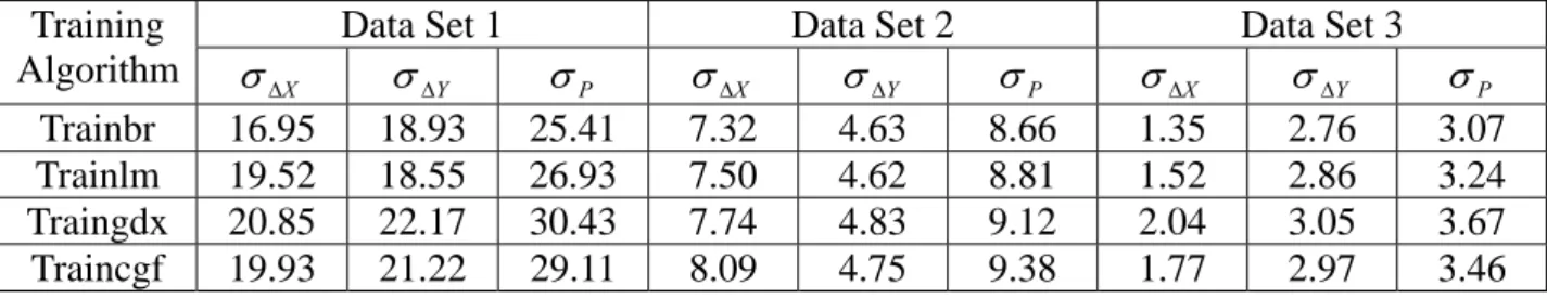
training algorithms were changed accordingly. The test results of data set 1 to 3 are shown in Table 1. The ‘training algorithm’ indicates the adopted BP ANN training algorithm. Four different training algorithms were tested: ‘trainbr’ (Bayesian regularization backpropagation), ‘trainlm’ (Levenberg-Marquardt backpropagation), ‘traincgf’ (Conjugate gradient backpropagation with Fletcher-Reeves updates), and ‘traingdx’ (Gradient descent with momentum and adaptive learning rate backpropagation) (Demuth and Beale, 2002).
From Table 1, it can be seen that the coordinate transformation accuracy, σ , of using the P ‘trainbr’ algorithm are ±25.41 cm, ±8.66 cm, and ±3.07 cm for data set 1 to 3 respectively, the minimal values of all cases. After considering accuracy of the BP ANN, the training algorithm “trainbr” was adopted in the following tests.
Table 1. Performance statistics of the BP ANN with varied training algorithms of data set 1-3. Data Set 1 Data Set 2 Data Set 3
Training Algorithm σ ΔX σ ΔY σ P σ ΔX σ ΔY σ P σ ΔX σ ΔY σ P Trainbr 16.95 18.93 25.41 7.32 4.63 8.66 1.35 2.76 3.07 Trainlm 19.52 18.55 26.93 7.50 4.62 8.81 1.52 2.86 3.24 Traingdx 20.85 22.17 30.43 7.74 4.83 9.12 2.04 3.05 3.67 Traincgf 19.93 21.22 29.11 8.09 4.75 9.38 1.77 2.97 3.46 5.3.2 The Coordinate Transformation Accuracies versus The Amount of Neurons in The
Hidden Layer Chosen in The BP ANN Program
In order to test the coordinate transformation accuracies versus the amount of neurons in the hidden layer chosen in the BP ANN program, the amount of neurons in the hidden layer was changed. After the so-called “trial and error” testing, the amount of neurons in the hidden layer of data set 1, 2, and 3 are 6, 3, and 13 respectively. The corresponding accuracies, σ , of data P set 1, 2, and 3 are ±24.63 cm, ±8.33 cm, and ±1.95 cm respectively.
5.3.3 The Coordinate Transformation Accuracy Comparisons with Other Coordinate Transformation Methods
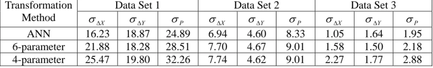
In order to test the coordinate transformation accuracy comparisons with other coordinate transformation methods, the same data sets (data set 1 to data set 3) were tested on other coordinate transformation methods, such as (1) 6-parameter Least Squares Adjustment, and (2) 4-parameter Least Squares Adjustment. The test results of data set 1 to 3 are summarized in Table 2. “ANN” denotes that BP ANN, with the “trainbr” training algorithm was used to estimate the check point’s TWD97 cadastral coordinates. The amount of neurons in the hidden layer chosen in the BP ANN programs of data set 1 to 3 were 6, 3 and 13 respectively according to the test results of the above-mentioned sections. “4-parameter” indicates that coordinate transformation equation (1) and Least Squares Adjustment approach were used to estimate the check point’s TWD97 cadastral coordinates. “6-parameter” indicates that coordinate transformation equation (2) and Least Squares Adjustment approach were used to estimate the check point’s TWD97 cadastral coordinates.
From Table 2, the σP values for “ANN”, “6-parameter”, and “4-parameter” of data set 1 are
± 24.89 cm, ± 28.51 cm, and ± 32.26 cm respectively. The σP values for “ANN”, “6-parameter”, and “4-parameter” of data set 2 are ±8.33 cm, ±9.01 cm, and ±9.01 cm
respectively. The σP values for “ANN”, “6-parameter”, and “4-parameter” of data set 3 are
±1.95 cm, ±2.18cm, and ±2.88 cm respectively. From Table 2, it can be seen that: (1) the performance of the cadastral coordinate transformation using the BP ANN was better than those of the other two coordinate transformation methods; and (2) if the test area is larger, then the performance of coordinate transformation using the BP ANN is better.
Table 2. BP ANN coordinate transformation accuracy comparisons with other coordinate transformation methods of data set 1-3.
Data Set 1 Data Set 2 Data Set 3 Transformation Method σΔX σΔY σP σΔX σΔY σP σΔX σΔY σP ANN 16.23 18.87 24.89 6.94 4.60 8.33 1.05 1.64 1.95 6-parameter 21.88 18.28 28.51 7.70 4.67 9.01 1.58 1.50 2.18 4-parameter 25.47 19.80 32.26 7.74 4.62 9.01 2.27 1.77 2.88 6 CONCLUSIONS
In order to study the cadastral coordinate transformation, algorithms of applying a back-propagation artificial neural network (BP ANN) were proposed. Three data sets, including 295 points around the Taiwan region, 56 points in Taipei City, and 44 points in Taichung City, were used to test the proposed algorithms. Based on the test results, the following comments can be made: (1) the training algorithm “trainbr” should be adopted in a BP ANN program; (2) the amount of neurons in the hidden layer chosen in the BP ANN program should be tested and adopted by trial and error; (3) the performance of the cadastral coordinate transformation using the BP ANN was better than those of the other two coordinate transformation methods; and (4) if the test area is larger, then the performance of coordinate transformation using the BP ANN is better.
ACKNOWLEDGEMENT
It is acknowledged that this research work was funded by the National Science Council with project No. NSC 95-2415-H-004-013-. Besides, the test data sets were kindly provided by the Satellite Survey Center, Department of Land Administration, Ministry of Interior, Taiwan, R.O.C.
REFERENCES
[1] Demuth, Howard. and Beale, Mark, 2002, User’s Guide of Neural Network Toolbox For Use with MATLAB, Version 4, The MathWorks.
[2] Wolf, Paul R. and Ghilani, Charles D, 2002, Elementary Surveying; An Introduction to Geomatics, 10th