一位元高精確度之載波相位估計及高運算效率之碼相位擷取

國 立 交 通 大 學

電信工程研究所

博 士 論 文

一位元高精確度之載波相位估計及高運算

效率之碼相位擷取

One-bit High-Accuracy Carrier Phase

Estimation and Computationally-Efficient

Code Phase Acquisition

研 究 生：謝 萬 信

指導教授：高 銘 盛

一位元高精確度之載波相位估計及高運算效

率之碼相位擷取

研 究 生: 謝萬信 指導教授: 高銘盛 博士

國立交通大學 電機資訊學院

電信工程研究所

摘要 本論文首先探討高精確度之一位元載波相位估計，我們根據訊雜比(signal-to-noise ratio, SNR)選擇合適的相位鑑別器，以達到高精確度的相位檢測。在低及高訊雜比的 環境中，反正切函數相位鑑別器(arctangent phase discriminator)以及雜訊補償數位相位

鑑別器(noise-balanced digital phase discriminator)分別可以精確地估測載波相位，但對

於中等訊雜比的應用，兩者皆有估計偏移(bias)的問題。因此，本論文提出訊雜比輔

助相位鑑別器(SNR-aided phase discriminator)，以解決中等訊雜比的相位檢測問題。

然而，許多實際的應用無法提供訊雜比的資訊，因此我們進一步將訊雜比輔助相位鑑

別器發展成同時估測相位及訊雜比的演算法。另一方面，本論文提出一個高運算效率

的碼相位(code phase)擷取方法，稱為相位同步擷取法(phase coherence acquisition,

PCA)。我們利用複數相量(complex phasor)擷取虛擬隨機序列(PN sequence)的碼相 位，其中輸入及本地序列會先分群，接著將分群序列映射到複數相量以提升抗雜訊能

力。由於相位同步擷取法主要利用複數相量之間的相位差，所以不需要複數乘法的運

算，因此相位同步擷取法所需的運算量遠低於習知的快速傅立葉轉換方法。最後，本

One-bit High-Accuracy Carrier Phase

Estimation and Computationally-Efficient Code

Phase Acquisition

Student: Wan-Hsin Hsieh Advisor: Dr. Ming-Seng Kao

Institute of Communication Engineering

College of Electrical and Computer Engineering

National Chiao Tung University

ABSTRACT

In the dissertation, we first investigate the high-accuracy one-bit carrier phase

estimation. Signal-to-noise ratio (SNR) is utilized to select the proper phase discriminator

to achieve high accuracy. The traditional arctangent phase discriminator (APD) and the

noise-balanced digital phase discriminator (NB-DPD) can obtain accurate carrier phase for

low and high SNR, respectively, but both algorithms have estimation bias in moderate

SNR. Therefore, the SNR-aided phase discriminator (SNRaPD) is proposed to obtain the

accurate phase. Since the SNR information may be unavailable in many applications, we

further extend the algorithm of SNRaPD to jointly estimate the phase and SNR. On the

other hand, we propose a computationally efficient method, termed Phase Coherence

Acquisition (PCA), for PN sequence acquisition by using complex phasors. In order to

combat noise, the input and local sequences are partitioned and mapped into complex

phasors in PCA. The phase differences between pairs of phasors are then utilized for code

phase acquisition, and thus complex multiplications are avoided. The computation load of

Acknowledgements

I wish to express my deepest gratitude to my advisor, Professor Ming-Seng Kao, for his kind guidance and assistance during my pursuit of my PhD degree. In addition to the inspiration for the subject matter and enthusiasm related to academic research, he also taught me a lot about life so that I will have an optimistic attitude toward every type of difficulty. It has been a great honor for me to work under his supervision. I am also deeply grateful to Dr. Chieh-Fu Chang, for his guidance on the presentation and publication of research results. His critical advices made the results more solid and convincing. He is also a great tutor who has guided me in the spirit of academic research. Without the invaluable support from Prof. Ming-Seng Kao and Dr. Chieh-Fu Chang, this work could not have been done.

Special thanks go to my laboratory colleagues and friends, Dr. Shu-Tsung Kuo, Dr. Fan-Shuo Tseng, Mr. Ching-Hui Lin (pylon), Mr. Hao-Tang Shih (archer), Mr. Chia-Feng Chang (dream), Mr. Shih-Wei Yeh (malaymo) and Mr. Wei-Chiang Chen for their encouragement and friendship during my study at NCTU. I would also like to thank all the friends in the NCTU Aboriginal club. They introduced me to a vivid and delightful life at NCTU.

I also thank Dr. Men-Tzung Lo for the opportunity to participate in his research projects. I learned a lot about biomedical signal processing under his guidance, for which also broadened my horizons on “signal processing”.

Finally, I greatly appreciate the encouragement and love of my parents, my parents-in-law and my wife, Waan-Rur Lu. Their warm consideration and understanding have accompanied me through this long journey.

Contents

Chinese Abstract

... I

English Abstract

... II

Acknowledgement

... III

Contents

... IV

List of Figures

... VI

List of Tables

... VII

List of Acronyms

... VII

Chapter 1

Introduction

1.1 Review of Phase Estimation Method ... 1

1.2 Review of Code Phase Acquisition Method ... 2

1.3 Organization of Dissertation ... 4

Chapter 2

One-Bit Accurate Phase Estimation

2.1 System Model ... 5

2.2 Accurate One-Bit Phase Discriminator ... 11

2.2.1 High-SNR ... 12

2.2.2 Low-SNR ... 13

2.2.3 Moderate-SNR ... 18

2.3 SNR-Aided Phase Discriminator ... 20

2.3.1 Proposed method ... 20 2.3.2 Cramér-Rao bound ... 23 2.3.3 Stop criterion ... 25 2.3.4 Range of application ... 27 2.4 Summary ... 30

Chapter 3

3.1 System Model ... 31

3.2 Nonlinear Least-Square Algorithm ... 34

3.3 Simulation and Discussion ... 36

3.3.1 Monte Carlo simulation ... 36

3.3.2 Range of application ... 40

3.4 Summary ... 42

Chapter 4

Code Phase Coherence Acquisition Method

4.1 Motivation ... 43

4.2 Acquisition by Phasor ... 44

4.3 Phase Coherence Acquisition Algorithm ... 47

4.3.1 Segmentation ... 47

4.3.2 Acquisition by Phase ... 49

4.3.3 Multi-layer PCA ... 52

4.3.4 Error detection capability ... 55

4.4 Performance of PCA ... 57

4.5 Computation of PCA ... 66

4.6 Summary ... 67

Chapter 5

Conclusions and Future Work

...69

Reference

...71

Appendix

A. Derivation of mean and variance of I-Q channel outputs ... 75

B. Power series representation of mean and variance of I-Q channel outputs .. 76

List of Figures

Fig. 2.1 System structure of one-bit SDR...6

Fig. 2.2 Relationship between the mean values of the I-Q channel outputs (first quadrant)...11

Fig. 2.3 Simulated results of NB-DPD regarding SNR...13

Fig. 2.4 Geometric representation of performance of APD on the I-Q plane...14

Fig. 2.5 Analytical and simulated results of APD regarding SNR...17

Fig. 2.6 Asymptotic performance of NB-DPD and APD regarding SNR...19

Fig. 2.7 Performance of SNRaPD regarding SNR...22

Fig. 2.8 MSE of SNRaPD (markers) and AvCRB (solid lines)...24

Fig. 2.9 Comparison between RMSE of SNRaPD and that of NB-DPD and APD...28

Fig. 3.1 RMSE of phase estimation...38

Fig. 3.2 Normalized RMSE of SNR estimation...38

Fig. 3.3 Mean I-Q correlation outputs for SNR between 0 to 15dB in 1dB step...39

Fig. 4.1 Schematic plot of the phase resolution for phasors on the complex domain...46

Fig. 4.2 Schematic plot of two layer segmentation: (a) segmentation in the 1st-layer; (b) segmentation of segment A in the 20 nd -layer...54

Fig. 4.3 Flow chart of the process of two-layer PCA...56

Fig. 4.4 Correct probability of d1 in the 1 st -layer of PCA...60

Fig. 4.5 Joint correct probability of d1 and c1 in the 1 st -layer of PCA...61

Fig. 4.6 STD of cˆ1 in the 1 st -layer of PCA when dˆ1d1...62

Fig. 4.7 Correct probability of d2 in the 2 nd -layer of PCA...65

Fig. 4.8 Joint correct probability of d2 and c2 in the 2 nd -layer of PCA...65

List of Tables

Table 4.1 Computations of the two-layer PCA and the FFT-based method...67

List of Acronyms

ADC analog-to-digital conversion

AGC automatic gain control

APD arctangent phase discriminator

AWGN additive white Gaussian noise

C/A coarse/acquisition

CRB Cramér-Rao bound

DPD digital phase discriminator

DSP digital signal processing

FFT fast Fourier transform

GNSS global navigation satellite system

I-Q inphase-quadrature

LEO low Earth orbit satellite

LLN law of large numbers

MLE maximum-likelihood estimation

MSE mean-squared error

NB-DPD noise-balanced digital phase discriminator

PCA phase coherence acquisition

PN pseudo-random

POD precise orbit determination

RMSE root mean-squared error

SDR software-defined receiver

SNR signal-to-noise power ratio

SNRaPD SNR-aided phase discriminator

STD standard deviation

TEC total electron content

Chapter 1

Introduction

Carrier phase estimation and code phase acquisition are essential in various applications,

such as the spread-spectrum system and the global navigation satellite system (GNSS) [1-2].

In modern applications, carrier phase estimation and code phase acquisition may be

implemented by means of the software-defined receiver (SDR) so as to obtain more

capability and flexibility in signal processing [3]. In SDR, more analog-to-digital conversion

(ADC) bits are generally desired so as to avoid significant quantization error. For example,

power degradation is at least 2dB for one-bit ADC [4-5]. On the other hand, because of the

benefits of the one-bit scenario, such as efficient bitwise processing and the avoidance of

automatic gain control (AGC), the one-bit ADC has still induced wide interest [6-11]. In this

dissertation, we investigate the high-accuracy one-bit carrier phase estimation for the tracking

process and propose a multiplication-free code phase acquisition method that uses much less

computation than the FFT-based method for SDR.

1.1 Review of Phase Estimation Method

For the conventional phase estimation of a sinusoidal carrier, the arctangent phase

discriminator (APD) is widely adopted since it achieves maximum-likelihood estimation

(MLE) in additive white Gaussian noise (AWGN) [12, page 167]. With infinite ADC bits, the

APD attains MLE irrespective of what the signal-to-noise ratio (SNR) is. However, this is not the case for realistic phase discriminators that have finite precision using a few-bit ADC,

especially those with one-bit ADC. The problem of parameter estimation for a single sinusoid

was previously investigated in [13-16]. In [16], Cramér-Rao bound (CRB) of one-bit

samples. The effects of one-bit sampling and quantization were also discussed. Unfortunately,

due to the lack of a closed form of probability mass function of samples [16, Eq. (10)], the

derivation of MLE of the sinusoidal carrier is intractable. Next, the dithering techniques were

used to improve the estimation performance. In [17] and [18], the asymptotic bias of one-bit

quantized mean estimation problems was addressed. Other relevant studies fell in the field of

the limiter phase detector [19][20, Chap. 10], which utilizes a limiter to prevent overload of

the received signal. For high SNR, the asymptotic phase estimation bias of APD had been

mentioned and an improved phase discriminator, called digital phase discriminator (DPD),

was proposed in [21]. The DPD achieves much higher asymptotic accuracy than that of the

traditional APD. However, the DPD does not perform well in low SNR environments due to

its sensitivity to noise. A modified DPD, termed the noise-balanced digital phase

discriminator (NB-DPD), incorporates the summation of noisy samples in phase estimation

leading to an improved noise performance [22].

1.2 Review of Code Phase Acquisition Method

Pseudo-random (PN) sequence acquisition is widely used in various applications. For

example, the acquisition is implemented to search for the correct code phase so as to identify

the transmitter in spread spectrum communications. Because of the limitations associated

with the hardware techniques, conventional code acquisition could only be achieved by

serially examining the possible code phase of the input sequence in the time-domain [23-24].

However, the time required for acquisition would be so long that limits the application of

longer PN sequence in practice. With the improvements in hardware implementation, the

parallel acquisition scheme, which employs a large amount of correlation circuits to examine

all the code phases concurrently was then devised to significantly reduce the acquisition time

[25]. A hybrid scheme had also been proposed to provide a compromise between the

[26]. In addition to the hybrid scheme, the acquisition schemes can employ auxiliary

subsystems, such as an auxiliary signal generator and a phase estimator, to attain reasonable

speed and complexity as well [27-28]. Owing to the recent development of digital signal

processing (DSP) for software receivers, the exhaustive computation of the direct serial

search between two sequences can be mitigated by fast Fourier transform (FFT) to reduce the

computation by utilizing convolution theorem [29-31], which states that the convolution of

two sequences can be derived from the pointwise product of corresponding Fourier

transforms (i. e., [ ]_{x n y n}[ ]_F _X( )_{ Y}( )_{ , where  denotes convolution and F} represents Fourier transform). The theorem that facilitates FFT can be used in the PN

sequence acquisition to efficiently search the code phase [32-33]. To further reduce the

computational burden of FFT-based acquisition, the efficient split-radix FFT techniques

rather than conventional radix-2 FFT could be used for transformation so that the number of

multiplications, addition and memory access can thus be reduced [34]. In addition, by the fact

that the more FFT points, the more computations are required, the acquisition with fewer FFT

points, which is cheaper, was performed on the coarse/acquisition (C/A) codes with

averaging up several samples of a code chip [35]. Instead of averaging the samples, the FFT

points could also be reduced by removing the insignificant points. By examining the

spectrum of input and local C/A sequences, it is found that most of the energy is contained in

the low-frequency half of the spectrum. Hence the other half of the spectrum, which is

comprised of very little information could be eliminated and thus the number points for

FFT-based acquisition were decreased [36]. On the other hand, the multiplication operation in

the FFT method generally requires many computational resources. Hence, a substitute

method employing Walsh transform (WT) was implemented to calculate the convolution

without the need for multiplications [37-38]. Specifically, as compared to the FFT-based

method, the WT-based method requires fewer additions and no multiplications, but additional

1.3 Organization of Dissertation

The dissertation is organized as follows. In Chapter 2, we investigate the one-bit

high-accuracy phase discriminator for three SNR ranges: low SNR, high SNR and moderate

SNR. Unlike traditional approaches, this approach first distinguishes which SNR range an

application falls into, and this SNR information is then utilized to select a proper phase

discriminator for achieving high accuracy. For low-SNR applications, traditional APD is

adopted. For high-SNR applications, NB-DPD is utilized to improve accuracy. Between

them, for moderate-SNR applications, a novel SNR-aided phase discriminator (SNRaPD)

developed using the nonlinear least-square method is proposed.

However, since the SNR information may be unavailable in many applications, the SNR

should also be estimated so as to attain the accurate phase estimation. Hence, a nonlinear

least-square algorithm for deriving the SNRaPD is further extended to jointly estimate the

phase and SNR estimation in Chapter 3. Because of the avoidance of AGC by using one-bit

ADC, the joint phase and SNR estimation method can accommodate signals with high

dynamic range. Potential applications for the spaceborne measurements are also discussed.

Next, we propose a novel method, termed the Phase Coherence Acquisition (PCA), to

search for the cross-correlation peak for pseudo-random (PN) sequence acquisition by using

complex phasors in Chapter 4. The PCA requires only complex additions in the order of N,

the length of the sequence, whereas the conventional method utilizing FFT requires complex multiplications and additions, both in the order of Nlog₂N . Specifically, the phase

differences between pairs of input and local phasors are utilized for acquisition, and thus

complex multiplications are avoided. The significant reduction of computational loads makes

the PCA an attractive method, especially when the sequence length of N becomes

extremely large which becomes intractable for the FFT-based acquisition. Finally, the

Chapter 2

One-Bit Accurate Phase Estimation

In this chapter, we clarify the accuracy of one-bit phase discriminators regarding SNR,

such as the accuracy of APD and NB-DPD in low and high SNR, respectively. Moreover, we

design an SNRaPD that utilizes the SNR information in phase estimation to enhance ultimate

accuracy in moderate SNR. A high-accuracy phase estimation is critical to the successful

tracking of carrier signals. In this study, the traditional inphase-quadrature (I-Q) structure

using one-bit ADC is studied first and the SNR-dependent mean value of the I-Q channel

output is derived. Note that, because the frequency of the received carrier can be captured by

the acquisition process or a frequency locked loop [2], the frequency shift between input and

local carrier can be regarded as a part of phase shift in steady-state tracking. Hence, the

influence of frequency shift is omitted and the AWGN channel is considered in our analysis.

Next, phase estimation with APD and NB-DPD are addressed. The SNRaPD is then

introduced and the improvement in accuracy is simulated and compared with the average

Cramér-Rao bound (CRB). In addition, an adequate stop criterion and the range of

applications regarding the SNR of SNRaPD are also discussed. The high-accuracy phase

information obtained with the proposed algorithm can potentially be applied to spaceborne

measurements in GNSS and beacon receivers when the ambient SNR falls within the

“moderate SNR” range and the multipath effect is mitigated.

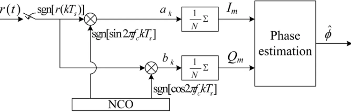
2.1 System Model

The system model for phase estimation of sinusoidal carrier in the one-bit SDR is shown

Fig. 2.1. System structure of one-bit SDR. ) ( ) 2 sin( ) (t f t t r   _c   (2.1) where f is the carrier frequency, _c  is an unknown phase, and (t) is the AWGN.

For phase estimation, the output frequency of the numerically controlled oscillator (NCO) is assumed equal to the incoming carrier frequency. Let T be the sampling period. The _s discrete-time one-bit quantized r(t) is given by

)] T ( ) T 2 sgn[sin( )] T ( sgn[ ] [k r k _s f k _s k _s r    _c   (2.2) where        . 0 if 1 0 if 1 ] sgn[ x x x

In addition, let the sampling frequency be f_s 1/T_s. We denote

p q h f f s c _{  (2.3)}

where h is the greatest integer less than or equal to f /_c f_s, and p and q are mutually

The mixer output of the inphase channel is given by s s sgn[ ( T )] sgn[sin 2 T ] sgn[sin( ) ] sgn[sin ] k c k k k a r k  f k           (2.4)

where _k 2f_ckT_s and _k (kT_s) is a zero-mean Gaussian random variable with variance _2_.

Consider p samples at tkT_s, k0,1,2,,p1. The normalized I-Q channel outputs are denoted by



        1 0 ] sgn[sin ] ) sgn[sin( 1 p k k k k p p I   (2.5a)



        1 0 ] sgn[cos ] ) sgn[sin( 1 p k k k k p _p Q   . (2.5b)

It can be proved that the samples of phases {₀,₁,,_p1} are uniformly distributed over )

2 , 0

[  with a separation of 2/p between neighboring  ’s [21]. Note that when we _i mention that p is “sufficiently” large later, it means that 2 /p is significantly smaller than the accuracy required for the estimation. According to Appendix A, the mean values and

variances of the I-Q channel outputs are given by

         





    [0, ) [ ,2 ) ) 1 P 2 ( ) P 2 1 ( 1     k k p k k I p (2.6a)          





     [0, /2) [3 /2,2 ) [ /2,3 /2) ) 1 P 2 ( ) P 2 1 ( 1       k k p k k Q p (2.6b)



     1 0 2 2 2 2 4 p _{P P} k k k Q I p p p   (2.7) where           ) sin( Q P k k dz z x x exp ₂ 2 1 ) ( Q



 2_         .

Note that the range of summation is defined according to the value of  in Eq. (2.6), and _k

k

P is a function of  . In Eq. (2.7), the variance of the one-bit quantized I-Q outputs _k consists of the effect of channel noise and quantization noise. Since {₀,₁,,_p1} are uniformly distributed over [0,2), the mean value of I-channel output in Eq. (2.6a) can be further derived by . ) sin( Q 2 ) sin( Q 2 1 2 ) sin( Q 2 ) sin( Q 2 2 1 ) , 0 [ ) 2 , [ ) 2 , [ ) , 0 [                                                  









                       k k k k p k k k k I p p p p (2.8)

From Eq. (2.1), the SNR of the sinusoidal signal is given by

2 2 1 SNR   . (2.9)

           





    [ ,2 ) [0, ) ) ) sin( ( Q 2 ) ) sin( ( Q 2 1         k k p k k I p (2.10) where   2SNR .

Suppose we choose f_s such that p is sufficiently large in Eq. (2.3). According to

Appendix B, the mean value of I-channel output of Eq. (2.10) can be represented as a power

series, which is given by







                       0 3 0 1 2 2 1 2 ) 2 1 2 cos( 1 2 ) 1 ( ) 1 2 ( 2 ! m m l l m m I _{m l} l m l m m m A p    (2.11) where _3/2 2 4   A .

Similarly, the mean value of Q-channel output of Eq. (2.6b) is denoted by

            





     [0, /2) [3 /2,2 ) [ /2,3 /2) )) sin( ( Q 2 )) sin( ( Q 2 1           k k p k k Q p . (2.12)

By a similar derivation of Eq. (2.11), the power series representation of _Q is given by







                       0 3 0 1 2 2 1 2 ) 2 1 2 sin( 1 2 ) 1 2 ( 2 ! ) 1 ( m m l m m m Q l m l m l m m m A p    . (2.13)

In addition, according to Appendix B, the power series of the variances of the I-Q channel

. ) 1 2 )( 1 2 ( 2 ! ! ) 1 ( 1 2 2 2 2 )) 1 2 ( 2 ! ( 1 2 2 4 2 1 0 1 3( ) 2 2 ) ( 2 0 3 1 2 2 4 2 2                                

 



              x y x x y y x y x m m m Q I y x y x y x y x m m m m p p p p      (2.14)

The above results are obtained for p samples. When the mean values and variances are generalized to N mp samples, where m is an integer, the normalized I-Q channel outputs are given by



      k k k k m N

I 1 sgn[sin( )  ] sgn[sin ] (2.15a)



    



k k k k

m _N

Q 1 sgn[sin( )  ] sgn[cos ]. (2.15b)

The mean values of the I-Q channel outputs are the same as Eq. (2.11) and Eq. (2.13),

respectively. The variance can be expressed as

. ) 1 2 )( 1 2 ( 2 ! ! ) 1 ( 1 2 2 2 2 )) 1 2 ( 2 ! ( 1 2 2 4 2 1 0 1 3( ) 2 2 ) ( 2 0 3 1 2 2 4 2 2                                

 



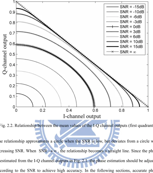
              x y x x y y x y x m m m Q I y x y x y x y x m m m m N N      (2.16)

The relationship between the mean values of the I-Q channel outputs is shown in Fig. 2.2.

Here, only the relationship in the 1st quadrant is illustrated because of the symmetry of the

trigonometric function. As can be seen in Fig. 2.2, the relationship between the I-Q channel

Fig. 2.2. Relationship between the mean values of the I-Q channel outputs (first quadrant).

The relationship approximates a circle when the SNR is low, but deviates from a circle with

increasing SNR. When SNR , the relationship becomes a straight line. Since the phase is estimated from the I-Q channel outputs in Fig. 2.1, the phase estimation should be adjusted

according to the SNR to achieve high accuracy. In the following sections, accurate phase

estimations regarding SNR are introduced. Note that, in order to evaluate the achievable

phase accuracy, the assumption of zero frequency offset is inherently applied to the following

analyses and simulations.

2.2 Accurate One-Bit Phase Discriminator

In this section, we introduce phase discriminators that have been proposed in the

literature, i.e., DPD [21], NB-DPD [22], and APD, for one-bit quantized data and discuss

2.2.1 High-SNR

When SNR, _k in Eq. (2.15) can be neglected. Moreover, when the number of samples N is large, by the law of large numbers (LLN), the I-Q channel outputs, denoted as

(I_m,Q_m), approximate their mean values, i.e., I_m _I and Q_m_Q . The relationship between the I-Q channel outputs is then denoted by

1   _Q

I 

 . (2.17)

The relationship is a straight line as shown in Fig. 2.2. In this situation, the phase can be

estimated by DPD, resulting in higher accuracy than that of APD [21]. Applying the system model of Fig. 2.1 in [21], the phase estimation according to (I_m,Q_m) is given by

) 1 ( 2 ) sgn( ˆ DPD  Qm Im   . (2.18)

The mean-squared error (MSE) of DPD will be negligible with a sufficiently large N.

However, in the high SNR environment, small noise variance still exists in the I-Q

channel outputs, and the relationship between the mean I-Q outputs deviates from a straight

line as shown in Fig. 2.2. Since DPD is sensitive to noise, the modified DPD, called

NB-DPD, is provided to improve phase estimation in this situation. The phase estimated by

NB-DPD is given by [22]           | | | | 1 2 ) sgn( ˆ DPD NB m m m m Q I I Q   . (2.19)

] ) ˆ [( E 2 DBD NB DPD NB  

 _  _  . Using Monte Carlo simulation methods for 100 trials,

DPD NB

 regarding SNR is shown in Fig. 2.3. As expected, _NBDPD decreases with increasing SNR. In addition, it decreases slightly with N in high SNR. Apparently, the

NB-DPD can achieve high phase estimation accuracy in high SNR.

2.2.2 Low-SNR

When the SNR is low, we have  1 in Eq. (2.11) and Eq. (2.13). Thus, the mean values of the I-Q channel outputs are approximated by

    cos 2 4 2 / 3  I , (2.20a)     sin 2 4 2 / 3  Q . (2.20b)

This proves the circular relationship of the I-Q channel output in the low SNR environment

as shown in Fig. 2.2. The result is also consistent with Pouzet’s conclusion, when we consider

a limiter as a binary quantizer with an infinite number of samples [19][20, Chap. 10]. Since

the mean I-Q channel outputs have an approximately circular relationship, APD is a good

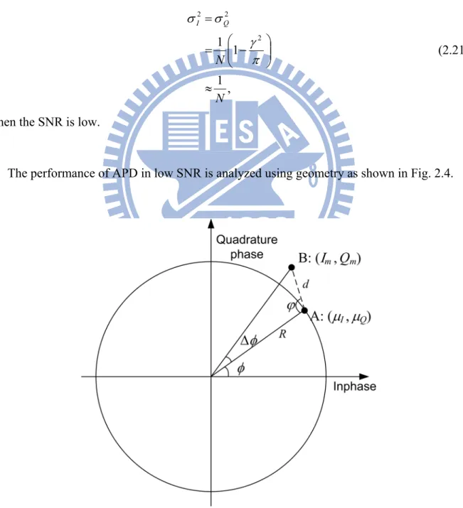
choice in low SNR. In addition, the variances of the I-Q channel outputs of Eq. (2.16) are

approximated by , 1 1 1 2 2 2 N N Q I               (2.21)

when the SNR is low.

The performance of APD in low SNR is analyzed using geometry as shown in Fig. 2.4.

First, let point A:(_I,_Q) denote the mean values of the I-Q outputs on a circle with radius

R and polar phase . According to Eq. (2.20), the radius R is given by

. SNR 4 2 4 2 / 3 2 / 3 2 2          _{I Q} R (2.22)

Next, let B:(I_m,Q_m) be the measured I-Q channel outputs. The distance between A and B is denoted by 2 2 _{( )} ) (I_{m I} Q_{m Q} d     . (2.23)

The sinusoidal carrier phase estimated from (I_m,Q_m) with APD is given by

   _        m m I Q atan2 ˆ APD (2.24)

where )atan2(x denotes the arctangent-2 function and  is the phase estimation error. 

Without loss of generality, let  0. From the law of sines, we have

) sin( sin   R d . (2.25)

Assume 1  . Then sin , and sin()sin() . Eq. (2.25) is approximated by

) sin(      R d . (2.26)

Suppose  is uniformly distributed over [0,). For a fixed d, the expected value of _{ }2

with respect to  is denoted by

. 2 ) ( sin 1 ] [ E 2 2 2 0 2 2 2 R d d R d    

_

       (2.27)

Assume d and  are mutually independent. According to the definition of variance and Eq. (2.21), the expected value of _{d is given by} 2

. 2 ] ) ( ) [( E ] [ E 2 2 2 2 2 N Q I d Q I Q m I m d            (2.28)

From Eq. (2.27) and Eq. (2.28), the MSE of phase estimation is denoted by

. SNR 16 1 2 ] [ E ]] [ E [ E 3 2 2 2 2      N NR R d d d    (2.29)

) degree ( . SNR 80 ) radian ( SNR 4 ]] [ E [ E 2 / 3 2 APD       N N d     _ (2.30)

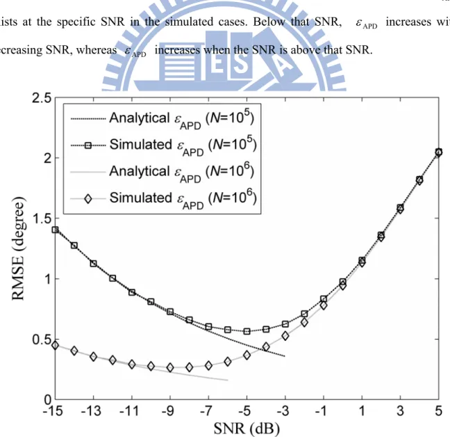
From Eq. (2.30), _APD is inversely proportional to the square root of the product of SNR and N. The analytical and simulated _APD are shown in Fig. 2.5. The simulated results are obtained by Monte Carlo simulation for 100 trials. From Fig. 2.5, the simulated results approach the analytical values in low SNR. Note that the analytical _APD is provided in part since the result is valid only when low SNR is assumed. From Fig. 2.5, a minimal _APD exists at the specific SNR in the simulated cases. Below that SNR, _APD increases with decreasing SNR, whereas _APD increases when the SNR is above that SNR.

According to Fig. 2.2, since the relationship of the mean values of the I-Q outputs deviates from a circle with increasing SNR, the increase in _APD is due to the estimation bias of the APD, which will be shown below.

2.2.3 Moderate-SNR

Between the high SNR and the low SNR, the relationship between the mean I-Q outputs

is complicated, as indicated in Fig. 2.2. The estimation bias of NB-DPD and APD is

examined by means of the asymptotic performance. Suppose N is sufficiently large. By LLN, the I-Q channel outputs of Eq. (2.15) approach their mean values, i.e., I_m _I and

Q m

Q  . The asymptotic performance of NB-DPD and APD are defined by

           | | | | 1 2 ) sgn( ˆ DPD -AsNB Q I I Q _{ }     , (2.31)        I Q   ˆ_AsAPD atan2 . (2.32)

The corresponding squared phase errors are given by 2 DPD -AsNB ND (ˆ ) e and 2 AsAPD A (ˆ )

e , respectively. We further denote the asymptotic estimation error by

2 / 1 ND DPD -AsNB (e )  (2.33) and 2 / 1 A AsAPD (e )  . (2.34)

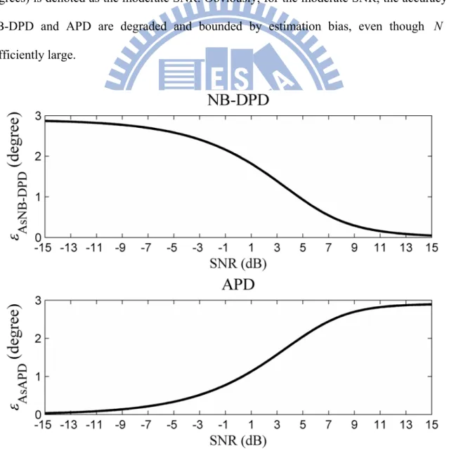
Note that the averaged values of e and _ND e_A, i.e., e and _ND e_A, are used in Eq. (2.33) and Eq. (2.34), since they are functions of . The _AsNB-DPD and _AsAPD regarding SNR are shown in Fig. 2.6. From Fig. 2.6, _AsNB-DPD and _AsAPD are small in high and low SNR, respectively. That is, _AsNB-DPD 0.1degrees if SNR12dB , and _AsAPD 0.1degrees when SNR-10dB. However, _AsNB-DPD becomes significant when the SNR decreases whereas _AsAPD becomes significant when the SNR increases. Here, the range of SNR in which both _AsNB-DPD and _AsAPD are not negligible is considered “moderate” SNR. For example, SNR between -10 dB and 12 dB in this case (phase accuracy requirement < 0.1

degrees) is denoted as the moderate SNR. Obviously, for the moderate SNR, the accuracy of

NB-DPD and APD are degraded and bounded by estimation bias, even though N is

sufficiently large.

Note that, even though the estimation error due to noise variance decreases with the square

root of the SNR in APD, as indicated in Eq. (2.30), the accuracy of APD is degraded because

of the estimation bias in moderate SNR. This result explains the degradation of _APD in moderate SNR as shown in Fig. 2.5. Above all, although NB-DPD and APD perform well in

high and low SNR, respectively, their performance is degraded by the estimation bias in

moderate SNR. Focusing on the moderate SNR, we develop an approach for reducing the

estimation bias and thus improving the accuracy in the following section.

2.3 SNR-Aided Phase Discriminator

2.3.1 Proposed method

Since the mean I-Q outputs vary with the SNR as shown in Fig. 2.2, the SNR should be

taken into consideration in achieving high-accuracy phase estimation. Therefore, the

SNRaPD is developed to improve the accuracy by using the SNR information. Let (_I,_Q) be the mean values of the I-Q output and (I_m,Q_m) be the measured I-Q channel output. In SNRaPD, we define a measure by

2 2 2 2 1 2 ( ) ( ) ( ) ( ( )) ( ( )) m I m Q L  I  Q            (2.35) where ₁()I_m _I, ₂()Q_m _Q, and  is the unknown phase to be estimated. In

addition, let T 2 1( ), ( )] [ ) (     

Λ , where ‘T’ denotes transpose and _L(_)_Λ(_)T_Λ(_)_.

When the SNR information is given,  is known, and the relationship of (_I,_Q) with respect to phase angle can be uniquely determined. When (I_m,Q_m) are given, suppose the most likely phase is what minimizes L() as follows:

)} ( min{ arg ˆ SNRaPD    L . (2.36)

This is the main idea of SNRaPD.

In optimization theory, the foregoing descriptions are known as the nonlinear

least-square problem. Newton’s method can be used to search ˆargmin{L()} [40]. The vector of the first derivatives of ₁() and ₂() is given by

T 2 1( ) ( ) ) ( _              d d d d J . (2.37) In addition, let ) ( ) ( ) ( ) ( ) ( ₁  h₁  ₂  h₂  H   (2.38) where 2 1 2 1 ) ( ) (     d d h  2 2 2 2 ) ( ) (     d d h  .

Then using Newton’s method,  is updated iteratively by

) ( ) ( )) ( ) ( ) ( ( T ₁ 1 1 1 1 T 1 1           _{i i i i i i} i    H     J J J Λ (2.39) where the _i denotes the phase obtained after the i-th iteration.

In SNRaPD, depending on the available SNR information, the initial phase ₀ can be estimated by NB-DPD or APD, and accuracy can then be improved iteratively by Eq. (2.39). The iteration will stop when |_i_i1| , where  is a small number. In the one-bit SDR

shown in Fig. 2.1, let the carrier frequency f_c 15.421111MHz, the sampling frequency MHz 096 . 4  s

f , and _{N 10}5_{. In this case, according to Eq. (2.3), we have p4096000}

and 2/p will be significantly smaller than the estimation accuracy described below. The performance of SNRaPD is evaluated by Monte Carlo simulation. In the simulation, the stop

criterion is _{ 10}3 _{degrees, and the estimated phase is given by}

i



ˆ_SNRaPD  . The RMSE defined by E[(ˆ )2]

SNRaPD SNRaPD  

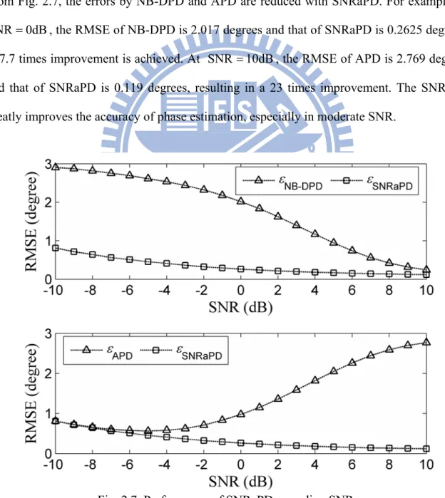
   is the average of 100 trials as shown in Fig. 2.7. From Fig. 2.7, the errors by NB-DPD and APD are reduced with SNRaPD. For example, at

dB 0

SNR , the RMSE of NB-DPD is 2.017 degrees and that of SNRaPD is 0.2625 degrees. A 7.7 times improvement is achieved. At SNR 10dB, the RMSE of APD is 2.769 degrees and that of SNRaPD is 0.119 degrees, resulting in a 23 times improvement. The SNRaPD

greatly improves the accuracy of phase estimation, especially in moderate SNR.

Regarding the number of iterations of Newton’s method in SNRaPD, normally less than four

iterations are required based on our simulation results. In addition, as mentioned in Section

2.2, NB-DPD and APD perform well in high and low SNR, respectively. Hence, fewer

iterations are required in SNRaPD when the initial phase is estimated by NB-DPD in high

SNR and by APD in low SNR.

2.3.2 Cramér-Rao bound

The CRB for one-bit quantized complex-valued signals was derived in [16]. The

performance of SNRaPD is compared with the CRB of the estimated phase. For simplicity, only the real-value case is considered. The probability mass function of r[k] in Eq. (2.2) is given by 2 2 0 ( ; ) Prob( [ ] 0; ) ( sin( )) 1 exp . 2 2 r k f q q r k r q dr                 _ _  



(2.40)

The Fisher information is then obtained by

1 0 1 1 2 0 1 I( ) ( ; ) ( ; ) ( ; ) 1 ( ; 1/ ) 2 N T r r k q r N k k f f q q f q                       

 



(2.41) where 2 2 2 2 )) sin( ) 2 / 1 (( erf 1 ) ( sin 1 exp ) ( cos 4 ) / 1 ; (                  _{  }       k k k k dt t x) 2 xexp( ) ( erf 0 2



   .

To investigate the achievable performance of SNRaPD, we assume that the frequency in Eq. (2.41) is zero, i.e. _k 0, and the phase is a uniform random variable. We define the average Fisher information by averaging Eq. (2.41) over phases, which is denoted by

2 0 2 1 I I( ) 2 ( 1/ ) 2 d N         



(2.42) where         ( ;1/ )d 2 1 ) / 1 ( 2 0



 .

Taking the inverse of the average Fisher information, we have the average CRB given by

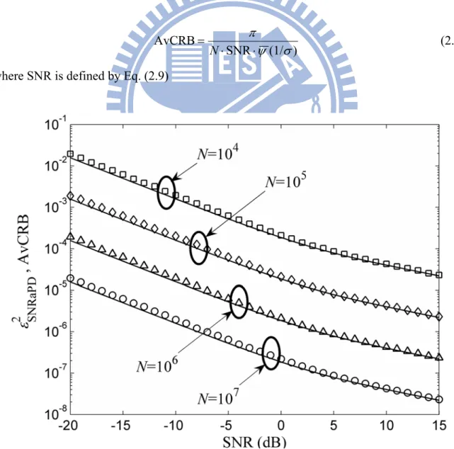
) (1/ SNR AvCRB       N (2.43)

where SNR is defined by Eq. (2.9)

The MSE of SNRaPD defined by E[(ˆ )2]

SNRaPD 2

SNRaPD  

   is compared with the AvCRB in Fig. 2.8. The AvCRB is plotted with solid lines, and the 2

SNRaPD

 is denoted by markers. The performance of SNRaPD is obtained from Monte Carlo simulation using 100 trials. In Fig. 2.8, 2

SNRaPD

 is close to AvCRB and their difference approaches zero with increasing SNR. Thus the accuracy of SNRaPD is validated. Note that the difference between AvCRB and 2

SNRaPD

 is similar for different values of N.

2.3.3 Stop criterion

As mentioned at the end of Section 2.3.1, although estimation bias is reduced by

SNRaPD, and ˆ_SNRaPD argmin{L()} is achieved by Newton’s method, noise variance still exists in ˆ_SNRaPD. As a result, the strict criterion 3

1| 10

|_i _i   (degrees) may result in the need for extra iterations, but the performance cannot be improved. From Eq. (2.35), the first derivative of L() is given by ). ( ) ( 2 ) ( ) ( ) ( ) ( 2 ) ( T 2 2 1 1               Λ J          d d d d d dL (2.44)

Note that the original criterion 3 1| 10

|_i _i   is consistent with dL(ˆ_SNRaPD)/d 0, since ˆ_SNRaPD argmin{L()}. As we consider the noise variance with Eq. (2.44), a new stop criterion is defined for SNRaPD as follows. Let  _c _c in Eq. (2.44), where _c is the true phase, and  is the phase error due to noise variance. Since the AvCRB of Eq. _c (2.43) is the theoretical bound of variance, let _c AvCRB. The new stop criterion is defined by | ) ( ) ( 2 | | ) ( ) ( 2 | T T c c c c i i       Λ  J  Λ  J . (2.45)

Note that the absolute value is used since the same result but with opposite polarity is

obtained by  _c_c . In addition, the criterion |2 ( )T ( )|

c c c c      Λ  J is a

function of _c, and the minimal value occurs when _c k/2. Hence, the criterion is further defined by _{|2 ( )}T _{( )| /2}      _{c c c c k} c     Λ

J to guarantee that the criterion is valid

for all phases.

Example―Determination of the stop criterion: Let SNR6dB, _{N 10}5_{, and 0}

c

 . According to Eq. (2.43), _{  AvCRB0.12215}

c  . Applying _{  0.12215} c c    to

Eq. (2.44), we have |2_J(0.12215)T_Λ(0.12215)|_0.001712_{. Hence, the iteration will stop} when 001712|2 ( )T ( )|_0.

i i 

 Λ

J .

A similar RMSE is achieved with the new stop criterion according to the simulation

results, which confirms our supposition. Moreover, the number of iterations is reduced with

the new criterion. Recall that the original criterion is consistent with dL(ˆ_SNRaPD)/d 0. Since Newton’s method will reach the criterion of ( )/ 2| T( ) ( )|

c c c c d dL   J   Λ   before that of dL(ˆ_SNRaPD)/d 0, the number of iterations is reduced accordingly.

Finally, most computational loads of SNRaPD fall in computing ₁() and ₂() as well as their derivatives, which involve  and _I _Q of Eq. (2.11) and Eq. (2.13), respectively. In practice, we use M terms to approximate  and _I _Q rather than infinite sums. Moreover, we can calculate and store coefficients in a table in order to further mitigate

the computational burdens. For applications with SNR less than 0 dB, M 8 is sufficient to well approximate  and _I  with RMSE smaller than _{Q 10}6_{. In addition, less than four}

iterations are normally required from our simulation results. Therefore the computational

burden of SNRaPD is feasible, given today’s fast processors.

2.3.4 Range of application

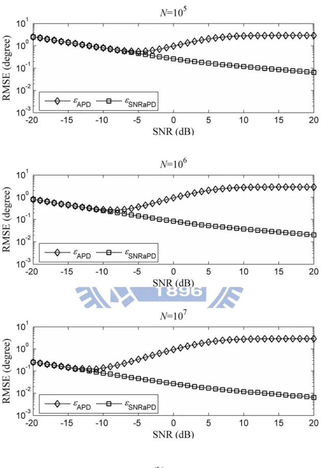
The range of application of SNRaPD is studied by comparing _SNRaPD with _NBDPD and

APD

 . The simulated results regarding SNR and N are illustrated in Fig. 2.9. From Fig. 2.9(a), compared with NB-DPD, the improvement in the accuracy of SNRaPD is significant

in moderate SNR. Note that the range of the moderate SNR may vary according to N and

the required phase accuracy for different applications. Moreover, in _{N 10}5 _{and N 10}6

cases, the improvement is negligible when the SNR is above 12 dB and 17 dB, respectively.

As N increases to _{10 , SNRaPD can consistently improve the accuracy to some degree for} 7

SNR below 20 dB. Similarly, in comparing SNRaPD with APD, the accuracy is greatly

improved in moderate to high SNR as shown in Fig. 2.9(b). The improvement is negligible

when the SNR is below -4 dB, -8 dB, and -12 dB, respectively. The above discussion

illustrates the superiority of the proposed SNRaPD in “moderate” SNR. As the ambient SNR

is increased to the “moderate” range, SNRaPD can potentially be used and provide improved

accuracy in spaceborne measurement techniques, such as the total electron content (TEC)

measurements on a beacon receiver or the precise orbit determination (POD) on a GNSS

receiver [41-45]. For example, when _{N 10}6 _{and SNR 0dB on the 400 MHz beacon}

signal, the phase error is 0.08 degrees and 0.94 degrees for SNRaPD and APD,

respectively. The estimation error of SNRaPD is approximately an order better than that of

APD. If more samples are utilized, the superiority of SNRaPD over APD remains significant

(b)

2.4 Summary

In this chapter, the high-accuracy phase estimation for one-bit SDR is investigated. We

propose the SNRaPD using the SNR information to reduce the estimation bias and achieve

the high-accuracy phase estimation. The mean values and variances of the I-Q channel

outputs in one-bit SDR are given by Eq. (2.11), Eq. (2.13) and Eq. (2.16), and the

SNR-dependent relationship of the mean I-Q channel outputs is explicitly shown in Fig. 2.2.

For high-accuracy phase estimation, NB-DPD can be used in high SNR as shown in Fig. 2.3.

For the low SNR, APD is selected according to Eq. (2.20), and its performance is illustrated

in Fig. 2.5. However, according to the asymptotic performance of NB-DPD and APD as

shown in Fig. 2.6, the estimation bias becomes significant and can have a negative impact on

the accuracy in moderate SNR. Focusing on this SNR range, we proposed SNRaPD using

Newton’s method to reduce bias and improve the resulting accuracy as shown in Fig. 2.7. The

accuracy of SNRaPD is certified by comparing the MSE with the AvCRB in Fig. 2.8. In

order to conserve computation time, an adequate stop criterion for SNRaPD with respect to

the noise variance is also defined by Eq. (2.45). Finally, the range of the application of

SNRaPD is investigated by comparing the associated RMSE with that of NB-DPD and APD

as shown in Fig. 2.9. Potential applications of SNRaPD and the corresponding performance

on SNR 0dB are also discussed. Nevertheless, the proposed SNRaPD requires the knowledge of SNR which is not available in many applications. Hence the joint phase and

Chapter 3

Joint One-Bit Phase and SNR Estimation

Generally, the SNR information is crucial for the quality control of the observed data [2,5]. Moreover, according to the results of chapter 2, the accurate SNR information enables

the accurate phase estimation. Since the SNR information may be unavailable in many

applications, we extend the algorithm for SNRaPD to jointly estimate of the phase and SNR.

Because the signals are one-bit quantized, the designed method can accommodate high

dynamic range applications.

In the following, the signal model of one-bit quantized sinusoidal carrier and the I-Q

correlation structure are revisited and adopted for joint phase and SNR estimation first. Next,

the nonlinear least-square algorithm of SNRaPD is extended to iteratively derive the phase

and SNR estimation. The performance of the proposed method is then verified by Monte

Carlo simulations. In addition, the feasibility of the proposed method for applications in

GNSS and beacon receivers is also discussed.

3.1 System Model

Consider a carrier with amplitude A , frequency f and phase _c . When the signal is disturbed by AWGN, the observed wave is denoted by

) ( ) 2 sin( ) (t A f t n t x  _c   (3.1) where n(t) is AWGN with zero mean and variance _2_.

2 2

2

  A . (3.2)

Note that Eq. (3.1) and Eq. (3.2) are different from their counterparts in chapter 2, i.e. Eq. (2.1) and Eq. (2.9), respectively, only on the amplitude A . When x(t) is one-bit quantized and sampled with period T , we have _s

] ) sin( sgn[ )] T ( ) T 2 sin( sgn[ ] [ k k s s c n A k n kf A k x           (3.3)

where _k 2kf T_{c s} and sampling frequency follows the property of Eq. (2.3).

For parameter estimation, assume that the frequency f is known and the local I-Q _c

components are sgn[sin_k] and sgn[cos_k], respectively. After one-bit quantization, ]

[k

x is then multiplied by local I-Q components, and summed to have the I-Q correlation outputs denoted by



  k k k x I [ ] sgn[sin (3.4) ]



  k k k x Q [ ] sgn[cos . (3.5) ]

Similar to Eq. (2.5), we consider p samples at tkT_s, k0,1,2,,p1 in I-Q correlation outputs, where p is specified in Eq. (2.3). The normalized I-Q outputs from these samples

are expressed by 1 0 1 sgn[ sin( ) ] sgn[sin ] p p k k k k I A n p      



   (3.6)

1 0 1 sgn[ sin( ) ] sgn[cos ] p p k k k k Q A n p      



   . (3.7)

According to Appendix A, the mean values of Eq. (3.6) and Eq. (3.7) are denoted by









[ ,2 ) [0, ) 2 Q 2 sin( ) Q 2 sin( ) p k k I k k p                  _    _ 





 (3.8)









[ / 2,3 / 2) [0, / 2) [3 / 2,2 ) 2 Q 2 sin( ) Q 2 sin( ) p k k Q _p k k                     _    _ 





 (3.9) where 2 1 Q( ) exp 2 2 x z x dz      _ _  



.

In addition, the variance of I-Q correlation outputs is given by



 



2 2 1 ₂ 2 0 4 Q 2 sin( ) Q 2 sin( ) . p p I Q p k k k p               _    _ 



 (3.10)

When the number of samples is generalized to N m p  and m is an integer, the I-Q outputs are denoted as I and _m Q , respectively. Let their mean value be _m  and _I _Q, respectively. It is easily proved that prove I and _m Q have the same mean values as _m I _p

and Q , i.e. _p p I I   and p Q Q

  . In addition, the variance of I and _m Q is given by _m



 



2 2 1 ₂ 2 0 4 Q 2 sin( ) Q 2 sin( ) . I Q N k k k N               _    _ 



 (3.11)

3.2 Nonlinear Least-Square Algorithm

After deriving the mean value of the I-Q correlation outputs, the nonlinear least-square algorithm is utilized to estimate the phase and SNR of the carrier. Let I and _m Q be the _m

I-Q outputs of one-bit quantized sinusoidal carrier. The phase and SNR of the carrier are

denoted by _{θ[,]}T_{, where the superscript ‘T’ denotes the transpose operation. Let}

) (θ

I

 and _Q(θ) be the mean values of I and _m Q regarding parameter _m θ , respectively. When the sampling frequency is carefully selected to have a large u , I and _m

m Q can be expressed by I I m I  (θ) (3.12) Q Q m Q  (θ) (3.13) where  and _I _Q are random variables in I-Q correlation outputs with variance given by Eq. (3.11).

To estimate the parameter θ, we construct a cost function as

2 2 2 2 1 2 T ( ) ( ( )) ( ( )) ( ( )) ( ( )) ( ) ( ) m I m Q f I Q y y          θ θ θ θ θ y θ y θ (3.14) where T 2 1( ), ( )] [ ) (θ θ θ y  y y .

The estimation of θ is denoted by

) ( min arg ˆ _θ θ f . (3.15)

Equation (3.14) and Eq. (3.15) form a nonlinear least-square problem. According to Eq. (3.14), the gradient of f(θ) is given by

) ( ) ( 2 ) (_{θ  J θ} T_{y θ} f (3.16) where )J(θ is the Jacobian matrix of y(θ).

In addition, the Hessian matrix of f(θ) is denoted by

)) ( ) ( ) ( ( 2 ) (_{θ J θ} T_{J θ H θ} F   (3.17) where )H(θ is the matrix whose ( qp, )-th element is given by



     2 1 2 j p q j j y y   .

The nonlinear least-square problem of Eq. (3.15) can then be solved, and θˆ is iteratively estimated by [40] ) ( )) ( ( 1 ) 1 ( ) ( _{θ F θ θ} θi _ i _  _f _{. (3.18)}

The iteration of Eq. (3.18) is stopped when _θ(i)_θ(i )1 _{, where  is a small number.} When the stop criterion is reached after the i-th iteration, the estimated result is given by

) (

ˆ _θi

θ . (3.19)

1) Initial value of phase

It is known that APD achieves MLE for discrete-time samples in a multi-bit scenario

[12]. For one-bit quantized data, although the accuracy may be degraded to some degree, the

initial phase of our approach can be readily determined by APD, which is denoted by

       m m I Q 1 -0 tan  . (3.20) 2) Initial value of SNR

After the initial phase is determined, let   for ₀ _I(θ) and _Q(θ) in Eq. (3.14). Then Eq. (3.14) is degenerated to be a function of . Subsequently, the initial SNR can be determined by searching the minimum value with respect to  in Eq. (3.14). The one-dimensional search technique, the Golden section method [40], is used to find the initial SNR, i.e. ₀. Note that the accuracy of ₀ is affected by the variance of ₀. Hence a loose stop criterion is used in the Golden section method to find the coarse ₀, and the computation time can be conserved.

3.3 Simulation and Discussion

3.3.1 Monte Carlo simulation

The Monte Carlo simulations are used to verify the joint phase and SNR estimation method, wherein each case of different SNR and N is tested for 1000 trials. Let

MHz 157 . 1  c

f and f_s 4.096MHz in the simulation, then p4096 according to Eq. (2.3). Assume ˆ is the estimated phase of the j-th trial, and _j  is the true phase. The root mean-squared error (RMSE) of phase estimation is defined by

2 / 1 1000 1 2 ) ˆ ( 1000 1 ) ˆ ( RMSE _       



 j j    . (3.21)

For SNR estimation, the RMSE is normalized to clarify the performance, which is denoted by

2 / 1 1000 1 2 ) ˆ ( 1000 1 1 ) ˆ ( nRMSE _       



 j j     . (3.22) where ˆ is the estimated SNR of the j-th trial, and _j  is the actual SNR.

In the nonlinear least-square algorithm of Eq. (3.18), the stop criterion is given by

0001 . 0 

 . In addition, for using the Golden section method to determine the initial SNR, a coarse resolution of 0.5 dB is used for the stop criterion. The one-bit ADC is commonly used

in low-power satellite applications. For potential applications on GNSS receivers, the

proposed method will be simulated for SNR as low as –30 dB. On the other hand, to illustrate

wide applicable range of our method, SNR up to 15 dB is also considered.

The performance of phase and SNR estimation are illustrated in Fig. 3.1 and Fig. 3.2,

respectively. Note that the RMSE of SNR is normalized and denoted by percentages. In Fig.

3.1, the RMSE of the phase is improved with increasing SNR and N . The phase RMSE’s

are below one degree when SNR is higher than –12 dB and –22 dB for _{N 10}5 _and 6

10 

N cases, respectively. Moreover, the accuracy of 0.1 degrees phase RMSE is achieved when SNR is higher than 12dB and –2dB in each case. According to Fig. 3.2, the SNR

estimation performs well in moderate SNR. Accurate SNR information can be used to learn

the achieved accuracy of phase estimation in this range. Specifically, the nRMSE is less than

10% for 21dBSNR13dB when _{N 10}5 _{and for 30dBSNR14dB when} 6

10 

N . Moreover, the estimation of SNR can be very accurate, i.e. nRMSE1%, when

6

10 

Fig. 3.1. RMSE of phase estimation.

Note that the nRMSE attains the lower bound when SNR is around 4 dB, and increases in

higher SNR. This phenomenon is investigated by plotting the mean I-Q outputs for

dB 15 SNR dB

0   as shown in Fig. 3.3. When SNR increases, the distance between neighboring curves becomes smaller and the distinction between them is little. Specifically,

for SNR4dB (dotted lines), the separations between the curves are recognizable. However, the distinction between curves becomes closer when SNR4dB (solid lines). Consequently, when slight variance occurs in the obtained I-Q correlation outputs for SNR

higher than 4 dB, the obtained I_m and Q_m will be fitted to _I(θ) and _Q(θ) with significant SNR error in the cost function of Eq. (3.14). Therefore, the performance of SNR

estimation becomes degraded. Especially, when SNR10dB , the curves are nearly overlapped, and the error in SNR estimation increases rapidly.

Recalling that the variance of I-Q correlation outputs is approximately inversely

proportional to N , the standard deviation (STD) will decrease with N . Hence, the

performance of the nonlinear least-square algorithm can be improved with N . This is consistent with the simulation results shown in Fig. 3.1 and Fig. 3.2. The results suggest that

N can be increased to compensate for the loss of amplitude information due to one-bit

quantization and the desired accuracy can be achieved.

3.3.2 Range of applications

GNSS receiver: For applications using carrier phase in GNSS receivers, the signal bandwidth is assumed to be 2 MHz concerning the coarse/acquisition (C/A) code. According to the

measured results of [46], when the elevation angles between 20° and 90° are of interest, SNR

from –30dB to –10 dB will be considered for different applications. According to the

simulation results of _{N 10}6_{, the phase RMSE’s of our method are 2.5545 and 0.25203}

degrees for SNR of –30dB and –10 dB, respectively. For L1 carrier (1575.42 MHz), these

errors correspond to 1.35 mm and 0.13 mm in length, and 1.73 mm to 0.17 mm for L2 carrier

(1227.6 MHz). Such performances are close to those of high-quality receivers [44, 46]. Note

that C/A code synchronization is assumed to be achieved before carrier phase estimation. In

addition, the nRMSE of SNR is less than 9% when _{N 10}6 _{and SNR is between –30dB and}

–10 dB. Regarding the potential application of POD in low Earth orbit satellites (LEO), the

accuracy of the orbit will be influenced by the satellite center variation, the attitude error, and

the antenna phase variation, which are at the centimeter level [47]. Our achieved phase

RMSE is much smaller than these variations. In addition, the phase RMSE is also

insignificant with respect to the ultimate accuracy after the orbit determination algorithm

reported in [47-49]. Hence, even though the proposed one-bit processing method is adopted,

the reported accuracy of POD in literatures can still be achieved. Furthermore, the quality of