貝式模型平均法在預測分析之應用 - 政大學術集成

全文

(1)國⽴立政治⼤大學統計學系研究所. !. 碩⼠士論⽂文. !. Graduate Institute of Statistics National Cheng Chi University. Taipei, Taiwan 116, R. O. C. ! Master Thesis ! ! ! 政治大⾙貝式模型平均法在預測分析之應⽤用立 ! ‧ 國. sit. !. y. 郭東穎. er. io. Kuo aTung-Ying iv l C n h e!n g c h i U !. n. !. ‧. !. Nat. ! !. 學. THE APPLICATION OF BAYESIAN MODEL AVERAGING FOR PREDICTIVE ANALYSIS. 指導教授：翁久幸博⼠士. !. Advisor：Prof. Ruby C. Weng. ! ! !. 中華民國103年6⽉月 . !. !. June, 2014 .

(2) ! . 謝辭首先要感謝是我的指導教授，翁久幸教授，從碩一下開始，不論是發想研究方. 向或是討論相關主題，她都給了我很大的空間做發揮。藉由老師的循循善誘，啟發學生獨立思考、找尋答案的求知慾，老師亦師亦友般的討論模式，更讓我勇於嘗試，不斷琢磨改進，體會到學術研究紮實的過程。翁老師平時對於學生的生活點滴，也十分關心，在困難的時候給予鼓勵，在無助的時候給予方向，師者，傳道、授業、解惑也。不僅授業解惑，更重要的是老師傳達給我們的態度與關懷，在我心中，她絕對是不可或缺的導師，也是人生中的貴人。 . 再者，我要感謝我的家人，尤其我的父母親，從小到大，給了我良好的環境學. 政治大每次在電話中聽到父母親的叮嚀與問候，頓時便充滿動力，繼續為研究衝刺，對父立習以及獨立思考、做決定的空間。在研究的過程中，他們不斷鼓勵我，盡力而為，. 母的感激，點滴心頭，實在非隻字片語所能形容。而我的弟妹，也給予我很大的幫. ‧ 國. 學. 助，每次回到家中，弟弟總是用他天真的笑容化解我平時的壓力，妹妹也會和我討. . ‧. 論生活與工作的經驗，對於我未來的想法提供意見。 . 而我要也要感謝政大，感謝六年政大生涯中，教過我的老師們，統計系扎實的. y. Nat. io. sit. 訓練，商學院豐富的課程，有了先前的學業基礎，才有機會完成這篇論文。也謝謝. er. 政大統研所的同學們，從碩一開始修課，大家一起奮鬥，一起討論，一起運動。無. n. a. v. l C 中大家成為一個大家庭，研究室的酸甜苦辣，都對我的研究過程產生蝴蝶效應。其 ni. hengchi U. 中，正憲、志軒、柏華是我參加資料採礦比賽的隊友，在他們身上我學習到很多，了解到團隊精神的真諦，很感謝他們這群好同學這兩年的陪伴。 . 最後，我感謝我的高中同學們，包含我的室友啟鳴，和我一同修習企管所的行. 銷研討，放膽學習另一個領域的新知，獲益良多。還有高中同學定衡、信宇、書賢，很難想像新竹高中的一群同學，會在臺北聚首，對於研究一同鞭策勉勵，對於生活一起排憂解悶，因為他們，我的研究所生涯的每一頁都充滿光彩與記憶。 . ! ! . .

(3) CONTENTS!. ! !. !. 中文摘要............................................................................................I Abstract…………………….…………………………………………….II Chapter 1 Introduction. 1 Chapter 2 Analysis Method……………………………………….…….2 2.1 Bayesian Model Averaging Method……………………….…2 2.2 Logistic Regression……………………………………………5 2.3 Assessment Review………………………….………………..6 政治. 大. Chapter 3 Practical Application .…………………………………..…..8 立. ‧ 國. 學. 3.1 The application of CARVANA case..….….…………………..8 3.2 Data preprocessing…….……….….………………………….9. ‧. 3.3 Data partition and sampling………………..………………..11 . y. sit. Nat. 3.4 Decision-making cut point…………………….……………..12. er. io. 3.5 Bayesian Model Averaging Analysis…………………….…18. n. 3.6 Predictive Performance………………………………………23 a iv. l C hengchi Un Chapter 4 Concluding remarks…..…..…………….………………..26 References……………………………………………………………..28. ! ! ! ! ! ! ! ! !.

(4) List of Figures!. ! ! Figure 1.!. Precision and Recall (Sensitivity)…………………………………………………6!. Figure 2.!. Data Partition and Cross-Validation……………………….……………………11!. Figure 3. !. Simulation of cut point in BMA model (F1-measure)…………………………13!. Figure 4. !. Simulation of cut point in BMA model (F0.5-measure)……………………….13!. Figure 5. !. Simulation of cut point in BMA model (F2-measure)…………………………14!. Figure 6. !. Simulation of cut point in full GLM model (F1-measure)……………14!. Figure 7. !. Simulation of cut point in full GLM model (F0.5-measure)………….15!. Figure 10. !. 治政 Simulation of cut point in Stepwise GLM model 大 (F1-measure).……………..16! 立 Simulation of cut point in Stepwise GLM model (F0.5-measure)……………16!. Figure 11. !. Simulation of cut point in Stepwise GLM model (F2-measure)…..………….17!. 學. !. y. Nat. List of Tables!. ‧. ! !. sit. Figure 9. !. Simulation of cut point in full GLM model (F2-measure)……………15!. ‧ 國. Figure 8. !. Table 2 !. The ability of model via AUC measure…………………………….……………8!. al. v i n Ch Variable Description……….………………..……………………………………10! engchi U n. Table 3!. er. Primary Biliary Cirrhosis example……………………………………………….2!. io. Table 1!. Table 4!. Models in different model selection strategies…………………….….……….21!. Table 5!. Comparison of parameter estimates for the variables in different models…22 !. Table 6!. The Predictive Performance Of Complete BMA Examples…………….…….24!. Table 7 !. The Predictive Performance Of Complete GLM examples……………….…..24!. Table 8!. The Predictive Performance Of Stepwise GLM examples……………………25!. Table 9!. The Predictive Performance Result In 100 Simulations………………………25!. Table 10!. BMA and Stepwise examples……………………………………………………25!. ! !. !.

(5) 中文摘要 . !. 當論及二元變數的分類問題，邏輯斯迴歸模型是個常用的典型模型。傳統的邏. 輯斯模型建置，往往會面臨模型選擇的問題，其方法例如逐步迴歸 (stpewise) 選取法。然而，在這種以單一模型作為最終架構的方式可能會遇到某些困難；例如模型不確定性，以及當多個模型在選取準則方面皆表現良好，而難以抉擇該使用何者為最終模型的問題。在本文中，我們引入貝式模型平均法 (BMA) 作應用，希望不僅能夠降低這些問題的影響，並且期望能夠增進模型在預測上面的表現，此外，透過 Occam’s window以及Laplace近似法，能夠將貝式模型平均法方法中較複雜的運算變得容易且更有效率。最後，我們對CARVANA的車輛資料做實證分析，運用了交叉驗. 政治大以及未做選取法來建立模型，進而比較。從實證結果顯示，在F-measure的評估架構立證模擬決策點、以及誤差抽樣等分析技巧，分別針對貝式模型平均法、逐步選取法. ‧ 國. 學. 下，貝式模型平均法以及精確率 (precision) 的表現較佳，而逐步迴歸 (stpewise) 選取法則在回應率的 (recall) 上的表現較佳，說明BMA方法不僅能夠改善先前的問題且在. ‧. 某些情況下，能夠提升模型預測上面的精確性。 . n. er. io. sit. y. Nat. al. Ch. engchi. I. i n U. v.

(6) ! ABSTRACT !. ! Tung-Ying Kuo,. Advisor: Prof. Ruby C. Weng.. Department of Statistics, National Cheng Chi University, Taipei City, Taiwan. !. ! Logistic regression serves as a classical model to be used when it comes to the. binary classification problem. In logistic regression, it is common to choose one model by some selected process such as stepwise method. However, using single model structure would confront with some problems such as model uncertainty and the difficulty in choosing among the models when they perform similarly. In this thesis, we aim to take. 政治大. uncertainty into consideration and refine the predictive performance via Bayesian Model. 立. Averaging (BMA). BMA, which considers all possible models, attempts to solve the. ‧ 國. 學. uncertainty by rendering the posterior probability of models as the weight to average. Additionally, Occam’s window and Laplace approximation would be employed to be more efficient in calculation process. Finally, Cavana vehicle auction data would be. ‧. demonstrated and applied by BMA method, stepwise model and full one. Equipped with. y. Nat. the techniques including under-sampling and cutting-point simulation. For the. io. sit. performances of F-measures and precision, BMA method is better. While stepwise model. n. al. er. work out for recall assessment. The result unveils that Bayesian Model Averaging. i n U. v. approach not only makes up model uncertainty but also enhances the precision of prediction in some situations.!. ! ! ! ! ! ! ! ! ! ! !. Ch. engchi. KEY WORDS: logistic regression; model uncertainty; Occam’s window; Laplace. approximation; Bayesian model averaging; Cross validation; Cut point; F-Measure . II.

(7) 1. Introduction Thanks to the improvement of technology, people are easier to get data that they need. The critical key to survive and be successful pivots on how to transform the data into information. Model-construction serves a path to understand the pattern and information in the data. Regression model is a common tool in statistical domain. There are two main contexts for building regression model: purely predictive research and data-oriented exploratory research. As mentioned by Breiman (2001), there are two goals in analyzing the data: one is PREDICTION and the other is INFORMATION. In this thesis, it is focused more on predictive work which is to figure out the model for good precision of prediction. We would like to solve the issues during the model construction process and seek to improve the predictive performance.. 政治大 terms a common practice to build model. The constructing process of typical logistic model 立 contains model selection which is usually implemented by stepwise or forward approach. Based on the target of binary classification problem, traditional logistic regression. ‧ 國. 學. However, this practice would trigger some problems: the risk of ignoring other possible models since the inference of the predictors only relies on the final model. Some previous. ‧. analytical examples to demonstrate this concern can be reviewed in Miller (2002), Regal. y. Nat. and Hook (1991), Madigan and York (1995), Raftery (1993), Kass and Raftery (1994) and. sit. Draper (1995). The oil-price example in Draper (1995) noted that a group of experts. er. io. provided 10 econometric models to forecast the price of oil but none of them was accurate. al. v i n C h that the posterior revealed e n g c h i U probabilities. n. because of the presence of scenario uncertainty, model uncertainty and predictive uncertainty. This oil example. make weaker. influence for effects than P-values does. Furthermore, the paper pointed out that the selection via P-values arguably overstates the evidence for an effect. Aside from model uncertainty, similar performance of possible models may be another issue. Sometimes, when building the model, several models fit the data well. In Raftery’s paper, the Primary Biliary Cirrhosis example (Dickinson, 1973; Grambschet al., 1989; Markus et al., 1989; Fleming and Harrington, 1991) shows that the performances of BIC criterion are similar from each other. It makes the decision-maker hard to choose the optimal single model. Five models with the top BICs are shown in Table 1. According to the result in this example, the top BIC model was not the most reasonable one.. ! !. 1/30.

(8) TABLE 1 Primary Biliary Cirrhosis example Mode lno.. 1 2 3 4 5. age. Edem a. Bili. Albu. UCo pp. V V V V V. V V V. V V V V V. V V V V V. V V V V. V. SGO T. Prot hro mb. V V. Hist. V V. V V. BIC. -174.4 -172.6 -172.5 -172.2 -172. Based on the difficulties mentioned, The BMA method (Hoeting et al., 1999), which belongs to ensemble method, is provided to solve some concerns by combining a bunch of models.. 政治大 averaging is applied widely. For example, random forest which combines a bunch of 立 decision trees works well in predictive performance for predictive problem. Bayesian. On the other hand, for many classification problem competitions, the idea of model. ‧ 國. 學. Model Averaging (BMA) is also a method by averaging a bunch of models. Thus, a problem was derived and could be researched: Does BMA method also have better. ‧. predictive performance in classification problem than traditional logistic model? In this thesis, we would apply BMA method and other statistical techniques to a. y. Nat. sit. practical data. After constructing models for the data, the under-sampling and cross-. al. er. io. validation approaches were used to enhance the achievement. Finally, the predictive. !. n. performance would be compared by precision, recall and F-measure.. Ch. engchi. i n U. v. 2.1 BAYESIAN MODEL AVERAGING METHOD! Traditional Bayesian model provides a model selection way to choose one model via comparing the Bayesian criteria of the models. However, referring inferences to the single model alone may be risky and could draw plausible inferences since the presence of information dilution. (Leamer, 1978, page 91). Equipped with the idea of Bayesian factor, Bayesian Model averaging, which combines all the models with posterior probabilities, was provided and developed. (Hoeting et al., 1999). 2/30.

(9) There are K models (means all possible models which is up to K =" 2 p ) taken into consideration. Assume M＝{" M 1 , M 2, ..., M K } is the model set and " Δ is the quantity of interest and p is the number of parameters. The posterior distribution given data D is. !. K. Pr(Δ D) = ∑ Pr(Δ M k , D)Pr(M k D). ! !. (1). k=1. The posterior probability for model " M k is given by:. !. Pr(M k | D) =. !! !. 立. where. Pr(D | M k ) = ∫ Pr(D | β k , M k )Pr(β k | M k )d β k. !!. (3)!. ‧. !. 政治大. ‧ 國. !. (2). ∑ l=1 Pr(D M l )Pr(M l ) K. 學. !. Pr(D M k )Pr(M k ). is the integrated likelihood of model " M k , " β k is the vector of parameters of model " M k , ". sit. y. Nat. " Pr(β k | M k ) is the prior density of " β k under model " M k , " Pr(D | β k , M k ) refers to the. al. The posterior mean and variance of " Δ are displayed as following:. ! ! ! ! ! ! ! where " Δˆ !. n. !. er. io. likelihood, " Pr(M k ) is the prior probability that " M k is the true model.. Ch. K en gchi. i n U. v. E(Δ D) = ∑ Δˆ k Pr(M k D). (4). k=0. K. Var(Δ D) = ∑ (Var[Δ D, M k ] +Δˆ k 2 )Pr(M k D) − E( Δ D)2. (5). k=0. k. = E(Δ D, M k ) , (Raftery, 1993; Draper 1995). As mentioned before, there would exist a risk when the model was based on one. single model structure. For example, the model selection criteria of backward and stepwise approaches work well but the predictive results are very different. In equation 4. 3/30.

(10) and 5, the BMA method averaging over all the models decreases the risk of model uncertainty issue since all models are taken into consideration. In BMA method, there are two main issues that we would confront and should deal with carefully: decision of prior distribution assignment and the complex calculation for Bayesian system probabilities. First, one involves the assumption of prior distribution in models. Different prior probabilities of models may cause disparate results. However, in practical, with a scarcity of information, One reasonable way is to set the prior probabilities " Pr(M k ) to follow a uniform distribution which means " Pr(M 1 ) = Pr(M 2 ) = ... = Pr(M K ) = 1 / K . In contrast, the prior probabilities could be modified if there were more understanding for the prior distribution. On the other hand, the difficulty of calculation of integrated probability could be conquered via Laplace method. Refer to the equation 3, it could be expressed as the following:. !. log Pr(D M k ) ≈ log Pr(D β!k , M k ) − dk log n. ‧ 國. 學. !. 立. 政治大. (6). ‧. where " dk is the number of parameter in Model k and n means the observation quantity. This approximation is also relevant to BIC (Schwarz Bayesian Information Criterion).. sit. y. Nat. Additionally, Occam’s window could help the user to reduce the number of models and make it more effective. The idea is to compare the highest posterior model probability. io. n. al. er. in equation (5) with every other model considered. It’s common to set the threshold to be. i n U. v. 20. In other words, is to keep the models which no less than 1/20 times than the highest. Ch. engchi. posterior one into following calculation. This concept can be expressed as the following:. ! !. ⎧ ⎫ max l Pr(M l D) A = ⎨M k : ≤ C⎬ Pr(M k D) ⎪⎩ ⎪⎭. !. (7). where the remaining models, belong to A subset of all models, should be taken into BMA calculation process. And C is the threshold recommended to be 20. By these two simple approaches, we could not only avoid the complex calculation but also make it more acceptable and efficient for practical use. Other advanced method such as MCMC could be used as well, but we don’t want to invest too much effort into this calculation part here.. 4/30.

(11) Thanks to the efforts of the predecessors, there are many direct ways to carry out BMA model process. In this material, we adopt Package ‘BMA’ built by Raftery et al. for R software as our tool. The following example would mainly be carried out by bic.glm and predict.bic.glm.!. 2.2 LOGISTIC REGRESSION! !. Since we attempt to deal with binary classification problem, Logistic regression is. frequently used since it is linear combinations of the predictors with weights indicating the variable importance. Thus, we would briefly introduce the Logistic regression model. Logistic regression model form can be expressed as the following:. Pr(Yi =1) ln(Ε[Yi x1,i ,..., xm,i ]) = ln( ) = logit(Pr(Yi =1)) = β 0 + β1 x1,i + ...+ β m xm,i Pr(Yi =0). 政治大. ! (8). ! 立 where Y belongs to binary response variable (Y=1 or Y=0) which indicates occurrence ‧ 國. 學. and non-occurrence respectively. Pr(Y =1) is the probability that Y =1 and Pr(Y =0) is the probability that Y=0. " x1 , x2 ,..., xm are predictors and " β 0 , β1,..., β m are regression. ‧. coefficients. i indicates the observation order.. al. n. !. y. sit. io. Odds(Yi = 1) = eln[odds(Yi =1)] = eβ0 +β1x1,i +...+β m xm,i. er. !. Nat. Here comes the result converted by logit(Y) form:. Ch. engchi. i n U. v. (9). And it can be expressed to another form to meet our target requisition:. !. β + β x +...+ β x. e 0 1 1,i m m,i Pr(Yi =1)= β + β x +...+ β x 1+ e 0 1 1,i m m,i. (10). According to the result in equation 10, Logistic regression model would produce the probabilities that the response variable equals to 1. With these probabilities, the predictive decision would be determined by comparing with cut-point. The cut point means where the probability of the positive judgement will be. It will be judged as “positive” when " Pr(Yi =1) is bigger than cut-point, while it will be noted as “negative” when " Pr(Yi =1) is lower than. 5/30.

(12) cut-point. It is common to set the cut-point as 0.5 but it could be adjusted according to requirement. We would discuss more details in chapter 3.. 2.3 ASSESSMENT REVIEW According to primary purpose of this thesis is to make forecasts for the future. How to evaluate the performance of prediction would be an issue. In this case, the bad purchase record served as “positive”, and the good purchase one served as “negative”. In classification problem, two terms are used frequently: PRECISION and RECALL. The precision for a model means the number of true positive divided by the total number of units labeled as belonging to positive class. On the other hand, the recall means the number of positive divided by the total number of units which actually belong to positive. 政治大 divided by total population, is立 used to evaluate the model as well. To understand more class. Last, ACCURACY is calculated by the sum of true positive and true negative. about the calculation and relation of these assessments, please take figure 1 as. ‧. ‧ 國. !. 學. reference.. Nat. y. Figure 1 : Precision and Recall (Sensitivity). er. io. sit. condition. n. negative apositive iv l C n hengchi U. test outcome. positive. negative. true positive. false positive. false negative. true negative. precision=!. Σ True positive Σ Test outcome positive. accuracy=. recall (sensitivity) =. Σ True positive Σ Conditional positive. !. precision =. Σ True positive + Σ True negative Σ Total population. True positive True positive + False positive. 6/30. (11).

(13) ! !. recall =. True positive True positive + False negative. (12). Aside from these fundamental assessment measures, For some cases, F-measure is also applied for classification problem since it’s difficult to make a choice between high precision and good recall. In short, F-measure is a hormonic mean of the precision and recall. This measure could not only consider precision and recall together but also modify the weight by the loss ratio of false negative to false positive. By setting different weight " β for the F-measure, the performance might be different for the model. The function is shown below. (13). 立. 學. ! !. 治 ⋅ recall 政2 precision Fβ = (1+ β 2 )⋅ β ⋅ precision大 + recall ‧ 國. !. In this case, we would employ " F0.5 , " F1 , and " F2 to evaluate and compare the. ‧. performance of different models. " F0.5 implies that users focus more on precision than recall. " F2 is used when recall is emphasized rather than precision.. Nat. sit. y. The final subtle measure used to compare the models would be AUC. The AUC is. io. er. defined as the area under the Receiver Operating Curve (ROC). Confronted with the binary classification task with m positive examples and n negative ones. To set " x1 , x2 ,..., xm. al. n. v i n to be the outcomes of the model on and " y , y ,..., y Cpositive U h e n gexamples i h c of the model on negative examples. The AUC is given by:. ! !. 1. ∑ ∑ AUC = m. n. i=1. j=1 xi >y j. mn. !. 2. n. to be the outcomes. 1. (14). which is related to the quality of classification. It could serve as a measure based on the pairwise comparisons between the classifications of two groups. It could be expressed to estimate the probability " Pxy that the model ranks a randomly chosen positive example higher than a negative example. Equipped with perfect ranking, AUC would equal 1 since all positive cases are ranked higher than negative ones. The expected AUC value for a. 7/30.

(14) random rank model is 0.5. The standard of performance suggested by Hosmer and Lemeshow (2000) is revealed in Table 2.. !. TABLE 2 The ability of model via AUC measure. AUC. The distinguish ability of model. AUC<0.6. Poor. 0.6<AUC<0.7. Normal. 0.7<AUC<0.8. Good. 0.8<AUC<0.9. Great. AUC>0.9. Amazing. 立. 政治大. 3.1 THE APPLICATION OF CARVANA CASE. ‧ 國. 學. !. There are many competitions of data analysis. Especially big data analytics have. ‧. been prevalent recently. One of the competition websites called Kaggle (http://. y. Nat. www.kaggle.com) has veteran experience. For the binary classification problem, we. io. sit. searched the previous competitions in Kaggle and found that CARVANA data is interesting. n. al. er. and the number of observations is immense enough. CARVANA company (http://. i n U. v. www.carvana.com/ ), which is touted as a 100% online car buying American company and. Ch. engchi. provides potential car buyers the opportunity to browse, finance and purchase a car online, offers a data about used-car auction records. Accordingly, it is the patented 360 degree photo system to capture the interior and exterior of each car that impresses customers for CARVANA website. People from time to time often confront a risk of fraud when purchasing a used car. The community calls the customers who involved in unexpected bad purchasing “Kicks”. According to the data provided by CARVANA, we sought to construct a model so that users can prevent the cars with issues from being sold. These car records belong to class-imbalanced data, which means that the sample size of some class dominates over others. In this case, the binary response variable. 8/30.

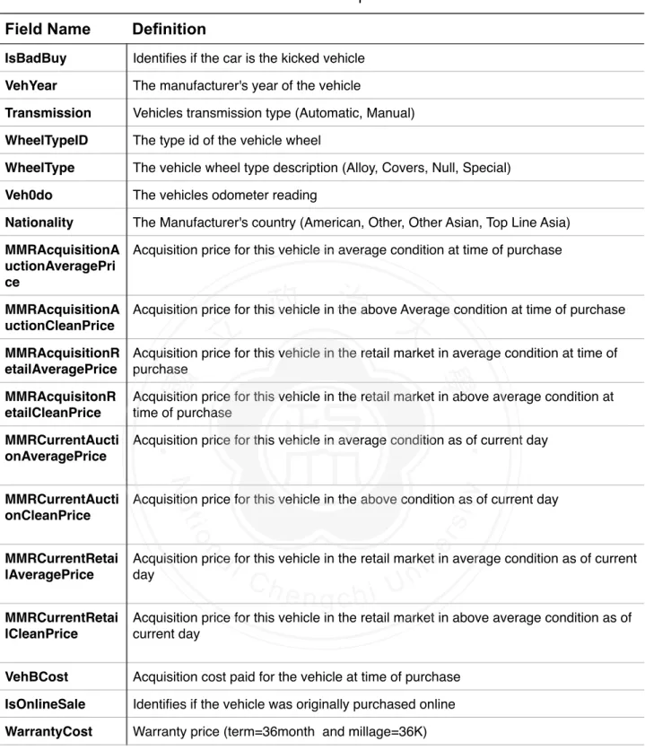
(15) named IsBadBuy is highly unbalanced. The majority part which means good-purchase accounts for 64,007 and the minority one which means bad-purchase has 8,976 samples.. 3.2 DATA PREPROCESSING There raw data contained 72,983 trade records including 34 variables. According to the complete-data rule, the observations with too many null values would be eliminated. The remaining 72,970 trade records would be employed in the following analysis. Before the feature extraction, the binary response variable and 33 predictive features were collected in this CARVANA data. After observing the data inputs and exploring the influences on response, we found that not all the predictive features are useful. Some predictive features such as RefID,. 政治大. PurchDate, Auction, VehYear, Model, Trim, Color, Make, PRIMEUNIT, AUCGUART, BYRNO,. 立. and VNST were eliminated since it contains too many missing-values, same information as. ‧ 國. predictive features into the final data set (shown in Table 3) .. 學. other features, or all values in the feature are identical. As a result, we selected 17. ‧. Finally, to re-calibrate the mistyping value in some features. For example, “Covers” are written as “COVER”. And continuous variables were standardized so that we might. sit. y. Nat. enhance the quality of prediction. Additionally, all the category variables were re-coded as factors (dummy-variable) to meet the software requisition.. io. n. al. er. In this process, 72,970 trade records would be used to construct the model of. i n U. v. CARVANA via 17 predictive features including categorical and continuous data form.. !. (Dickinson, 1973; Fleming and Harrington, 1991; Grambsch et al., 1989; Leamer and Leamer, 1978; Markus et al., 1989; Miller, 2002; Regal and Hook, 1991). Ch. engchi. ! ! ! ! 9/30.

(16) TABLE 3 Variable Description Field Name. Definition. IsBadBuy. Identifies if the car is the kicked vehicle. VehYear. The manufacturer's year of the vehicle. Transmission. Vehicles transmission type (Automatic, Manual). WheelTypeID. The type id of the vehicle wheel. WheelType. The vehicle wheel type description (Alloy, Covers, Null, Special). Veh0do. The vehicles odometer reading. Nationality. The Manufacturer's country (American, Other, Other Asian, Top Line Asia). MMRAcquisitionA Acquisition price for this vehicle in average condition at time of purchase uctionAveragePri ce. 政治大. MMRAcquisitionA Acquisition price for this vehicle in the above Average condition at time of purchase uctionCleanPrice. 立. ‧ 國. 學. MMRAcquisitionR Acquisition price for this vehicle in the retail market in average condition at time of etailAveragePrice purchase Acquisition price for this vehicle in the retail market in above average condition at time of purchase. MMRCurrentAucti onAveragePrice. Acquisition price for this vehicle in average condition as of current day. MMRCurrentAucti onCleanPrice. Acquisition price for this vehicle in the above condition as of current day. MMRCurrentRetai lAveragePrice. Acquisition price for this vehicle in the retail market in average condition as of current day. MMRCurrentRetai lCleanPrice. Acquisition price for this vehicle in the retail market in above average condition as of current day. VehBCost. Acquisition cost paid for the vehicle at time of purchase. IsOnlineSale. Identifies if the vehicle was originally purchased online. WarrantyCost. Warranty price (term=36month and millage=36K). ‧. MMRAcquisitonR etailCleanPrice. n. er. io. sit. y. Nat. al. Ch. engchi. ! ! 10/30. i n U. v.

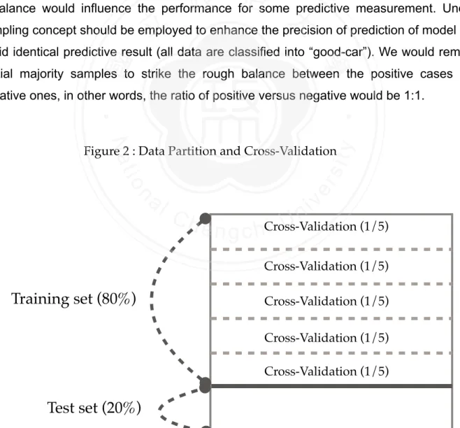
(17) 3.3 DATA PARTITION AND SAMPLING As Figure 2 reveals, we randomly split the data set into training set and test set so that we could be easier to evaluate the performance and over-fitting issue. With the 80-20 rule, the training set contained 58,376 trade records and the test set contained 14,594 ones. Additionally, since the positive responses (means bad-purchase record) account for only 13% for all, we kept the similar positive ratio for training and test sets. After the Data partition step, the training set would be split into five parts (Shown as Figure. 1). In this case, we would apply 5 fold cross-validation to find the decision-making cut-point. Therefore, each small part of training set had 11,675 records respectively. As described in 3.1, CARVANA data is highly class-imbalanced. Namely, the number of observations in major group is quite different from that in minority group. The. 政治大. imbalance would influence the performance for some predictive measurement. Under-. 立. sampling concept should be employed to enhance the precision of prediction of model and. ‧ 國. 學. avoid identical predictive result (all data are classified into “good-car”). We would remove partial majority samples to strike the rough balance between the positive cases and negative ones, in other words, the ratio of positive versus negative would be 1:1.. ‧ y. Nat. n. al. er. io. !. sit. Figure 2 : Data Partition and Cross-Validation. Ch. i n U. v. (1/5) i e n g c hCross-Validation Cross-Validation (1/5). Training set (80%). Cross-Validation (1/5) Cross-Validation (1/5) Cross-Validation (1/5). Test set (20%). 11/30.

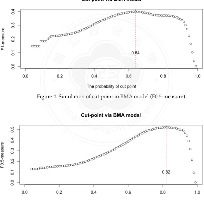
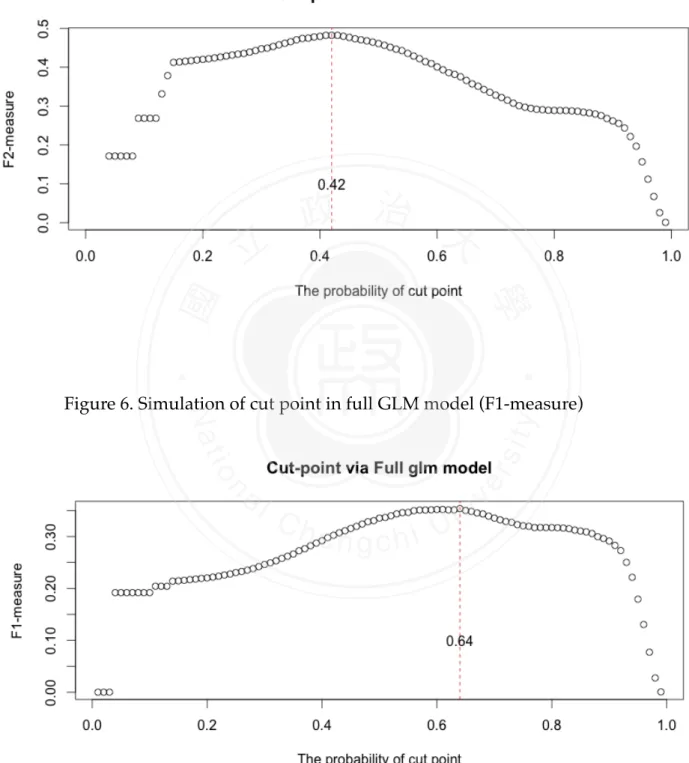
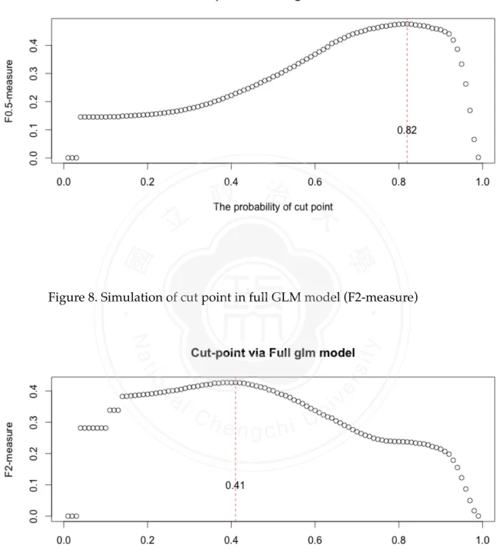
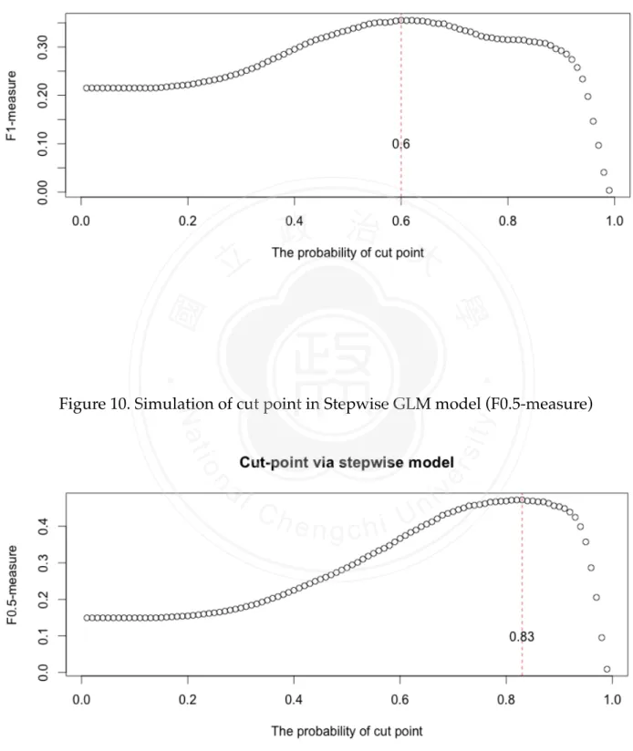
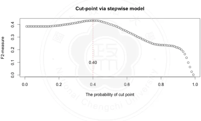
(18) 3.4 DECISION-MAKING CUT POINT As mentioned in this chapter 2, the cut-point can be modified according to the requirement. We would discuss how to choose the cut point to make decision. After we constructed the models and derived the probabilities of positive outcomes, the cases would be classified to be bad-purchase or good-deal. In general, the classified decisions would be made by probability 0.5. However, this approach might tip the balance (all cases were judged to be one majority group) or could not reach the top performance degree.! As Stone (1974) advocates, cross-validation technique can be used to get more predictive accuracy. Applied with the five-fold cross-validation data set, the simulation technique could be implemented to find out where the most appropriate cut point is for this data rather than 0.5. The steps of our practice are displayed as the following:. 政治大. To begin with, we split five data sets of training data; we constructed five models by. 立. different parts of data. For example, the first part would be tested by the model based on. ‧ 國. 學. second to fifth parts of training data. The second part one would be tested by the model constructed on 1st, 3rd, 4th and 5th parts of training data. And then 3rd, 4th and 5th parts are. ‧. in the same way. In this step, five models were derived toward each part. Next, the probability was set from 0.01 to 0.99. For this probability, every single. sit. y. Nat. classification matrix was built by comparing the predicted probabilities and the set. io. al. n. set classification matrix.. er. probability. And then five classification matrices would be combined to a complete training-. i n U. v. Finally, F-measure would be calculated by the complete classification matrix. Refer. Ch. engchi. to the simulation tool, the cut point to fit highest F-measure could be decided. In this thesis, we applied three models to the CARVANA data. Implemented by BMA model, full generalized linear model and stepwise generalized linear model. For BMA model, as Figure 3 to Figure 5 demonstrate, the cut points were set to be 0.64, 0.82 and 0.42 respectively. Based on these cut-points, we would employ them to assess the performance of prediction in different purpose. For full generalized linear model, as Figure 6 to Figure 8 suggest, the cut point were set to be 0.64, 0.82 and 0.41 respectively. Based on these cut-points, we would employ them to assess the performance of prediction in different purpose. For stepwise generalized linear model, as Figure 9 to Figure 11 suggest, the cut point were set to be 0.60, 0.83 and 0.40. 12/30.

(19) respectively. Based on these cut-points, we would employ them to assess the performance of prediction in different measurement. With stimulated cut points for each model, we could improve the performance of prediction and make better decision rather than traditional 0.5 threshold.. !. Figure 3. Simulation of cut point in BMA model (F1-measure). 立. 政治大. ‧. ‧ 國. 學 y. Nat. n. al. er. io. sit. Figure 4. Simulation of cut point in BMA model (F0.5-measure). Ch. engchi. ! ! 13/30. i n U. v.

(20) ! ! ! ! !. Figure 5. Simulation of cut point in BMA model (F2-measure). 立. ‧. ‧ 國. 學. ! ! !. 政治大. n. al. er. io. sit. y. Nat. Figure 6. Simulation of cut point in full GLM model (F1-measure). Ch. engchi. ! ! ! 14/30. i n U. v.

(21) 立. 政治大. 學. Figure 8. Simulation of cut point in full GLM model (F2-measure). ‧. ! ! ! ! !. Figure 7. Simulation of cut point in full GLM model (F0.5-measure). ‧ 國. ! !. n. er. io. sit. y. Nat. al. Ch. engchi. ! ! ! ! 15/30. i n U. v.

(22) ! ! Figure 9. Simulation of cut point in Stepwise GLM model (F1-measure). 立. 政治大. ‧ 國. 學. !. ‧. !. n. al. er. io. sit. y. Nat. Figure 10. Simulation of cut point in Stepwise GLM model (F0.5-measure). Ch. engchi. ! 16/30. i n U. v.

(23) ! ! ! ! Figure 11. Simulation of cut point in Stepwise GLM model (F2-measure). 立. 政治大. ‧. ‧ 國. 學. n. er. io. sit. y. Nat. al. Ch. engchi. ! !. (Monteith et al., 2011) (Berger and Delampady, 1987; Bradley, 1997; Breiman, 2001; Chen, Liaw and Breiman, 2004; Cortes and Mohri, 2004; Dietterich, 2000; Draper, 1995; Fernandez, Ley and Steel, 2001; Hoeting, Raftery and Madigan, 1996; Hoeting et al., 1999; Kass and Raftery, 1995; Kohavi, 1995; Lemeshow and Hosmer, 2000; Madigan and Raftery, 1994; Madigan, York and Allard, 1995; Merlise, 1999; Miller, 2002; Posada and Buckley, 2004; Raftery, 1996; Raftery et al., 2005; Raftery, Madigan and Hoeting, 1997; Stone, 1974; Tierney and Kadane, 1986; Tsao, 2014; Volinsky et al., 1997; Wang, Zhang and Bakhai, 2004; Wasserman, 2000; Zhu, 2004) . 17/30. i n U. v.

(24) ! 3.5 BAYESIAN MODEL AVERAGING ANALYSIS! After sampling and cut-point simulation steps, we would apply BMA method. to bad-car forecasting. Within the data set, 17 predictors are available to be used and the number of input variables is 21, including dummy variables. Interaction is ignored here since it took too much time for computing all the Bayesian combinations. By the bic.glm commend in “BMA” package in R, 4,194,304 model combinations (" 2 22 ) were taken into BMA computing consideration. With Occam’s Window rule mentioned before, there are 9 models with highest posterior model. 政治大 BMA model set. Among these models, one with highest posterior probability is 立 probabilities (cumulative posterior probability reach 0.999) were selected in final. 0.476. There are 5 to 8 predictive variables in each sub-model of BMA. Besides. ‧ 國. 學. BMA model, stepwise model contains 12 input variables and complete model without selection included 21 predictive variables. The mean of input variables and. ‧. selection results are shown in Table 4.. sit. y. Nat. As TABLE 5 reveals, the " P(β j ≠ 0 D) means that the posterior probability which the parameter effect doesn’t equal to zero given Data. It can be derived by. io. n. al. er. compute how much ratio the predictive variable account for across all the models,. i n U. v. The posterior means and posterior probabilities of the coefficients are also attached. Ch. engchi. in BMA model. Interpreting the effect of a particular predictive variable on the likelihood of occurrence of event can be expressed in the following ways.. ! !. Pr(β j ≠ 0 D) =. ∑ Pr(M. M k ∈A. k. D)* I k (β j ≠ 0). (15). where A means a set of models selected in Occam’s Window and " I k (β j ≠ 0) stands the indicator function which equals to 1 when the " β j is in model Mk and 0 otherwise. The interpretation of " P(β j ≠ 0 D) posterior probability is recommended to follow the rules provided by Kass and Raftery (1995). The rules are shown as follows:. !. 18/30.

(25) ! ! P(β j ≠ 0 D) <0.5. Poor evidence. 0.5! ≤ ! P(β j ≠ 0 D) <0.75. weak evidence. 0.75! ≤ ! P(β j ≠ 0 D) <0.95. Positive evidence. 0.95! ≤ ! P(β j ≠ 0 D) <0.99. Strong evidence. ! P(β j ≠ 0 D) ! ≥ 0.99. Very strong evidence. Next, The Bayesian point estimate (posterior mean) and standard error (posterior standard deviation) of are given by " β j are shown as:. !. ˆ Pr(M D) E(β j D)政 = ∑ β治 j k M k ∈A. 立. M k ∈A. j. D, M k ) + βˆ j 2 ]Pr(M k D)} − E(β j D)2. ! ! !. (16). (17). ‧. ‧ 國. ∑ {[var(β. 學. SE(β j D) =. 大. where " βˆ j is the posterior mean of " β j under model " M k . The difference between. Nat. sit. y. BMA method and stepwise method is that the point estimates are combined by all. io. er. possible effects and weighted with model posterior probabilities.. There are fifteen coefficients’ estimates in BMA final model, including. n. al. Ch. i n U. v. intercept, VehYear, WheelTypeID, WheelTypeDUMMY1, WheelTypeDUMMY2,. engchi. W h e e l Ty p e D U M M Y 3 , Ve h 0 d o , N a t i o n a l i t y D U M M Y 2 , MMRAcquisitionAuctionAveragePrice, MMRAcquisitionAuctionCleanPrice, MMRAcquisitonRetailCleanPrice, MMRCurrentRetailCleanPrice, VehBCost, IsOnlineSale, WarrantyCost. Aside from BMA model, we apply step command in R to build stepwise Logistic model. In stepwise model, the final model is selected by Akaike information criterion (AIC) in stepwise procedure. There are fourteen coefficients’ estimates in stepwise model. P-values are attached and they are all less than 0.1. AIC is defined in this command as " AIC. = - 2*log L + k * edf for large n, where L is the. likelihood, edf is the number of parameters in the model and k is the penalty term. 19/30.

(26) Table 4! Models in different model selection strategies. Bayesian Model Average STEPWISE COMPLETE. Mean or Percentage. 1. 2. 3. 4. 5. 6. 7. 8. 9. VehYear. 0.1776. T. T. T. T. T. T. T. T. T. Transmission. 0.0353. WheelTypeID. 2.8022. WheelType! DUMMY1. 0.3899. T. WheelType! DUMMY2. 0.1312. T. WheelType! DUMMY3. 0.0096. Veh0do. 0.0851. Nationality DUMMY1. 0.0041. Nationality DUMMY2. 0.1104. Nationality DUMMY3. 0.0524. MMRAcquisitionAu ctionAveragePrice. -0.1040. MMRAcquisitionAu ctionCleanPrice. -0.0500. MMRAcquisitionRe tailAveragePrice. 0.0248. MMRAcquisitonRet ailCleanPrice. 0.0657. MMRCurrentAuctio nAveragePrice. -0.1027. MMRCurrentAuctio nCleanPrice. -0.0520. T. MMRCurrentRetail AveragePrice. 0.0425. T. MMRCurrentRetail CleanPrice. 0.0747. VehBCost. -0.1076. IsOnlineSale. 0.0224. WarrantyCost. 0.0489. T T T. T. T. T. T. T. T. T. T. T. T. T. T. T T. T. T. 立. T. T. T. 政治大. T. T. T. T. T T. T. T. T. T. T. T T. ‧ 國. T. T. T. T. T. T. T. T T. T. ‧ T. T. y. T. T. n. al. er. sit. T. Ch. n U engchi. T. iv. T. T. T. T. T. T. T. T. T. 5. 7. 7. 8. 7. 7. 7. 7. 0.476 0.147 0.125 0.066 0.046 0.044 0.035 0.033 0.027. 20/30. T. T T. T. 6. T. T. T T. T. 學. T. io. Posterior model probability. T T. Nat. No. of variables. T. T. T. T. T. T. T. T. T. 12. 21.

(27) Table 5! Comparison of parameter estimates for the variables in different models BMA. Mean!. SD!. STEPWISE. P(β j ≠ 0 D) Coefficient. βD. βD. Intercept. -0.6234. 0.7850. 100. VehYear. 0.4408. 0.0233. 100. Transmission. COMPLETE. Pr(>|z|). Coefficient. Pr(>|z|). -2.17921. <0.0001. -1.8795. 0.0178. 0.42351. <0.0001. 0.4403. <0.0001. -0.0394. 0.6863. 0. WheelTypeID. 0.1459. 0.3868. 12.5. 1.07055. <0.0001. 0.9094. 0.0199. WheelType! DUMMY1. -0.2665. 0.0571. 85.3. -1.22247. <0.0001. -1.0227. 0.0092. WheelType! DUMMY2. 3.0679. 0.1152. 87.5. 0.7321. 0.5313. WheelType! DUMMY3. -0.2582. 0.6873. <0.0001. -1.8612. 0.0199. Veh0do. 0.1158. 0.0209. <0.0001. 0.1055. <0.0001. 0.0154. 0.5536. 0.0893. ‧. 0.0922. 0.1444. 0.0579. 0.5152. -0.0697. 0.0268. -0.0333. 0.2427. -0.0117. 0.6693. -0.0903. 0.0015. -0.1186. MMRAcquisitionAu ctionCleanPrice. -0.0015. 0. y. 0.0220. io. MMRAcquisitionAu ctionAveragePrice. -0.0057. 100. n. al. 0.0090. MMRAcquisitionRet ailAveragePrice MMRAcquisitonRet ailCleanPrice. 0.81518. 4.4. Nat. Nationality DUMMY3. 0.0305. 0. 0.0228. Ch. -0.12155. 3.3. e 0n g c h i U 7.3. sit. 0.0060. 0.11503. <0.0001. er. ‧ 國. Nationality DUMMY2. 100. 學. Nationality DUMMY1. 立. 政12.5 治-1.92850 大. v ni. -0.06157. 0.0269. MMRCurrentAuctio nAveragePrice. 0. -0.0005. 0.9875. MMRCurrentAuctio nCleanPrice. 0. -0.0335. 0.2371. MMRCurrentRetailA veragePrice. 0. 0.0151. 0.5833. MMRCurrentRetailC leanPrice. 0.0042. 0.0202. 4.6. 0.05629. 0.0465. 0.0878. 0.0023. VehBCost. -0.0985. 0.0214. 100. -0.12334. <0.0001. -0.1087. <0.0001. IsOnlineSale. -0.0069. 0.0468. 6.6. -0.29550. 0.0204. -0.3054. 0.0192. WarrantyCost. -0.0014. 0.0083. 3.5. -0.03673. 0.0636. -0.0151. 0.4846. 21/30.

(28) which equals to 2 corresponding to the traditional AIC. The maximum likelihood parameter estimates of the single model selected from the stepwise procedures. Thirteen coefficients’ estimates in stepwise model. In these two models, there are four predictor variables of 21 input variables (VehYear, Veh0do, MMRAcquisitionAuctionAveragePrice and VehBCost) are related to response variable significantly. The Bayesian posterior probabilities and P-values of stepwise Logistic regression model are matched and present strong evidences (" P(β j ≠ 0 D) " ≥ 0.99 and P-values<0.0001, respectively). Six predictors of all ones (Transmission, NationalityDUMMY3, MMRAcquisitionRetailAveragePrice, M M R C u r re n t A u c t i o n Av e r a g e P r i c e , M M R C u r re n t A u c t i o n C l e a n P r i c e a n d CurrentRetailAveragePrice) are suggested that there exists no relationship with. 治政 S e v e n p r e d i c t i v e v a r i a b l e s o f a l l p r e大 d i c t o r s ( W h e e l Ty p e I D , 立 WheelTypeDUMMY1, WheelTypeDUMMY3, MMRAcquisitonRetailCleanPrice, occurrence of bad-purchasing in both BMA and stepwise methods.. ‧ 國. 學. MMRCurrentRetailCleanPrice, IsOnlineSale, WarrantyCost) have weaker relationship with response variable via Bayesian posterior probabilities than P-values. Three. ‧. predictive variables of all predictors (WheelTypeDUMMY2, NationalityDUMMY2, MMRAcquisitionAuctionCleanPrice) partially agree there exists the effect toward the. y. Nat. er. io. (NationalityDUMMY1) is revealed partially in stepwise model.. sit. occurrence of bad-purchasing event in BMA approach. Only one input variable. al. v i n C h Our results U and effects of predictors. For example, e n g c h i suggest that considering all possible BMA sub-models, the Bayesian posterior mean for is 0.4408, presenting n. In Logistic regression, the coefficients of predictors reveal the importance. that an additional one standardized year increase, 55 percent (= exp(0:02×10)−1) increase in the odds of a bad-car purchasing event occurring. The main predictors selected in both BMA and stepwise approaches reveal similar estimates for the parameters. The close point estimates in BMA and stepwise show the similar exploratory information toward the predictor. Additionally, those variables partially appeared in BMA method speak volumes about a possible advantage of BMA. Even the relationship between the predictive variable and the response variable is weak, BMA method will take it into account.. 22/30.

(29) 3.6 PREDICTIVE PERFORMANCE! In order to assess the performance of BMA method for prediction, we would employ data partition mentioned in chapter 3.3 to use. Training set includes 58,376 trade records, and 14,360 samples (7,180 records are positive events) would be selected via undersampling technique in 3.3. Testing set contains 14,594 records and 1,795 observations of them are bad-purchasing records. Based on cut point simulated by cross-validation process in 3.4, we would apply the data in training set to construct BMA, stepwise and complete models to compare the performance of prediction. The data in training set was used to identify the relationships between predictors and bad-purchasing events by using these three analysis methods. Then we compared these predictive performance of three models by calculating the F0.5, F1, F2 score with. 政治大. testing set. Additionally, the precision and recall for each model in Table 6 to Table 8 with. 立. the test data set. In these tables, the details of measurements are displayed for five times. ‧ 國. 學. in each model method.. Because the samples in training and testing sets might be different, it is reasonable. ‧. to implement these model procedures for many times and take the averaging results. Therefore, we took much time to run the computation process and Table 9 presented the. sit. y. Nat. averaging result of one hundred computer simulations.. As Table 9 suggests, no matter in F0.5, F1 or F2 measures, BMA model has slightly. io. n. al. er. better performance prediction. Since BMA has outstanding performance for precision of. i n U. v. prediction, the mean of F0.5 measure is better than the others. So does F1 measure and. Ch. engchi. F2 measure. Although BMA presents higher mean of assessments for this case, the variance of F-measures in BMA are not smaller than the others. AUC, which terms the distinguish ability of model, reveals good level for each model. All the AUC values are fallen in the 0.70 to 0.75. The most outstanding model is stepwise chosen model, the second is BMA model and the third is complete one. Often, there is a trade-off relationship between precision and recall. For example, If less positive test outcomes in A model than B model for the same cut-point, then the result of A model will have less False Positive, and more False Negative. Therefore, from the definitions of precision and recall, you'll see that the precision is likely (not always, because it also depends on the number of True Positive) to increase, and recall is likely to decrease. Accordingly, we can discover something interesting in our analysis. For this car. 23/30.

(30) data, equipped with F1-oriented cutting point, BMA method is the best in precision assessment, the second is complete model and the third is stepwise approach. Conversely, in recall, stepwise approach gives the greatest performance, the second is complete one and the third is BMA. The variances of precision and recall in complete model are larger than BMA and stepwise ones. The reason of this consequence might be explained as the following: Based on similar F1-oriented cut-points (both around 0.6) in BMA model and stepwise one, the positive test outcomes in BMA model were more than the ones in stepwise one. Namely, Less test outcomes were judged as kicked-vehicle in BMA than the ones in stepwise model. (shown in Table 10) Overall, the performance of prediction does not meet our expectation because of low precision and recall. The possible reasons may be the limitation of logistic regression (such as linear assumption) , ignoring the interaction of predictors and hazy-understanding. 政治大 consequence is matched. for car-domain knowledge. BMA, which belongs to ensemble method, shows better performance of F-measure. This. with the announcement:. better average predictive ability” noted by. 學. ‧ 國. “averaging over all the. 立 models provides. Madigan and Raftery (1994).. ‧. Table 6 The Predictive Performance Of Complete BMA Examples BMA. F0.5. 0.5050. 0.5099. 0.5113. 0.5055. F1. 0.3949. 0.3974. 0.4034. 0.4007. F2. 0.4695. AUC. 0.7417. Precision (F1). 0.4382. 0.4763. 0.4635. Recall (F1). 0.3593. 0.3409. 0.3571. AVG. 0.5077. 0.5079. 0.3947. 0.3982. 0.4761. 0.4728. 0.7429. 0.7406. 0.4340. 0.4686. 0.4561. 0.3721. 0.3409. 0.3541. er. io. BMA. y. BMA. sit. BMA. Nat. BMA. n. a0.4697 iv 0.4743 0.4745 l C n 0.7361h e n0.7431 g c h i U0.7394. Table 7 The Predictive Performance Of Complete GLM examples GLM(compl ete). GLM(compl ete). GLM(compl ete). GLM(compl ete). GLM(compl ete). AVG. F0.5. 0.5055. 0.4980. 0.5050. 0.5101. 0.5162. 0.5070. F1. 0.3955. 0.3880. 0.3919. 0.3788. 0.3916. 0.3892. F2. 0.4751. 0.4718. 0.4728. 0.4682. 0.4716. 0.4719. AUC. 0.7428. 0.7387. 0.7396. 0.7362. 0.7409. 0.7396. Precision (F1). 0.4484. 0.3871. 0.4445. 0.3461. 0.3690. 0.3990. Recall (F1). 0.3538. 0.3889. 0.3504. 0.4184. 0.4173. 0.3857. 24/30.

(31) Table 8 The Predictive Performance Of Stepwise GLM examples GLM(stepwi GLM(stepw GLM(stepwi GLM(stepwi GLM(stepwi se) ise) se) se) se). ! ! !. AVG. F0.5. 0.5106. 0.5041. 0.5067. 0.4946. 0.4980. 0.5028. F1. 0.3882. 0.3885. 0.3874. 0.3946. 0.3875. 0.3892. F2. 0.4698. 0.4784. 0.4745. 0.4755. 0.4713. 0.4739. AUC. 0.7359. 0.7445. 0.7410. 0.7445. 0.7401. 0.7412. Precision (F1). 0.3762. 0.3638. 0.3575. 0.3936. 0.3592. 0.3701. Recall (F1). 0.4011. 0.4167. 0.4228. 0.3955. 0.4206. 0.4114. 政治大 Table 9 . 立. GLM_full. BMA. Mean. SD. Mean. SD. F0.5. 0.5044. 0.0062. 0.5052. 0.0053. 0.0052. F1. 0.3908. 0.0056. 0.3904. 0.0049. ‧. 0.5056 0.3966. 0.0039. F2. 0.4738. 0.0028. 0.4735. 0.0026. 0.4740. 0.0027. AUC. 0.7415. 0.0035. 0.7388. 0.0027. 0.7411. 0.0030. Precision (F1). 0.3698. 0.4533. 0.0202. Recall (F1). 0.4117. 0.3574. 0.0128. n. er. io. a0.0156 l C 0.0130 h. sit. SD. Nat. Mean. y. GLMstepwise. 學. ‧ 國. The Predictive Performance Result In 100 Simulations. v i n 0.3868 0.0334 engchi U 0.3993. 0.0487. !. Table 10 BMA and Stepwise examples. BMA. Condition Positive. Test outcome. Stepwise. Negative. Positive. 647. 795. Negative. 1148. 12004. precision recall. Condition Positive. Test outcome. Negative. Positive. 720. 1194. Negative. 1075. 11605. 0.4486. precision. 0.3762. 0.3604. recall. 0.4011. 25/30.

(32) 4 CONCLUDING REMARKS! For data analysis, there are two main cultures mentioned by Breiman (2001). One is prediction-focused goal and the other one is explanatory. In this thesis, we are eager to focus on predictive goal in binary classification problem. Logistic regression, which serves as a common and simple model, was used and discussed. In traditional Logistic regression, analysts might confront with some issues as follows. For example, a model selection such as stepwise approach leads to a single ‘optimal’ model and then make inferences via this final model. However, this method critically ignores uncertainty. Besides model uncertainty, similar criteria seem to be another issue. A handy example demonstrating this dilemma will be the Primary Biliary Cirrhosis example noted in Raftery’s paper. The BIC criteria of models are similar but the performances are very different.. 立. 政治大. To apply Bayesian model averaging method to Logistic regression, we set all the. ‧ 國. 學. prior probabilities of possible models to be equal without expert information. Additionally, the Occam’s window and Laplace method were employed so that making the computing. ‧. process to be efficient. In this thesis, we applied the BMA model, traditional stepwise model and full one to CARVANA practical data. Since we sought to enhance the precision. sit. y. Nat. of prediction, the under-sampling technique and cutting point simulation were also used in each model. As the results of predictive performance suggests, no matter which F-. io. n. al. er. measure we choose, BMA slightly outperforms the stepwise method and the full model in. i n U. v. CARVANA data. Asides from the performances of F-measures, with the cutting point found. Ch. engchi. by F1-measure, BMA works better for the prediction. For the recall, stepwise method performs better. After confirming the test results in some simulations, the main reason for this consequence is that less test outcomes were judged as kicked-vehicle in BMA than the ones in stepwise model for CARNAVA data. In CARVANA example, besides the little improvement of predictive performance by BMA method, most of the significant point estimates in stepwise model are contained in BMA model. This result speaks volumes for the possible advantage of BMA method since it took possible models into consideration. As these models suggest, the predictors: the year and the odometer reading of the vehicle have the significant and positive influence on the occurrence of bad-purchasing. The acquisition average price and the cost paid at time of purchase are the only significant. 26/30.

(33) predictors in acquisition price indexes and they have negative effect. Other predictors are partially supported in one model. Most of them are partially significant and reveal strong evidence in stepwise one. This result is matched with the announcement: p-values arguably overstate the evidence for an effect even when there is no model uncertainty (Berger and Delampady, 1987). In addition to the purpose of predictive aim, BMA serves as a appropriate tool for exploratory goal for explanatory variables. The input variables, which partially left in the BMA model, suggest that there exists weak association with response variable. But there show no evidence in stepwise one. There is another clinical example demonstrating this claim could be referred in Wang, Zhang and Bakhai (2004). Consequently, with the approaches mentioned in this thesis such as cutting point simulation, analyst can follow and implement BMA model simply. There is no need to choose one model. It is possible to average the predictions from several models.. 政治大 prediction accuracy than a single model and dilute model uncertainty concern. 立 There are some issues we may consider and might modify in the future. Without Therefore, for practical classification problem, BMA method could achieve better. ‧ 國. 學. the expert knowledge of used vehicles, the ability of precision in our example seems not to meet our expectation (only about 0.4). If one is eager to enhance the precision of. ‧. prediction, The feature extraction work by domain-knowledge will be a critical step.. y. Nat. Second, the setting of prior distribution may influence the predictive performance. Next,. sit. the computing process in “BMA” package is approximated by Laplace method based on. er. io. simplicity. The accurate posterior probabilities of models can be computed by MCMC. al. method. And this approximation may affect the performance. Another concern is that only. n. v i n one practical data we applied for C analysis, dataUshould be applied to confirm the h e n gmore h c i improvement of BMA method.. Presented by Monteith et al. (2011) is Bayesian model combination (BMC). BMC, which model weights are modified in Dirichlet distribution, terms a correction to BMA. Although BMC is somewhat more computationally expensive than BMA, it is worth to try and compare this model in the future. Last but not least, the efficiency of computing may be another issue that analyst will concern. It took about 20 seconds to implement one BMA model and 8 minutes for the whole BMA comparing program. And one stepwise model took 50 seconds and 13 minutes to finish the stepwise comparing precess. Last but no least, full model took only 1 second to implement one model and 90 seconds to complete the whole process.. 27/30.

(34) REFERENCES! Berger, J. O., and Delampady, M. (1987). Testing precise hypotheses. Statistical science, 317-335.! Bradley, A. P. (1997). The use of the area under the ROC curve in the evaluation of machine learning algorithms. Pattern recognition 30, 1145-1159.! Breiman, L. (2001). Statistical modeling: The two cultures (with comments and a rejoinder by the author). Statistical science 16, 199-231.! Chen, C., Liaw, A., and Breiman, L. (2004). Using random forest to learn imbalanced data. University of California, Berkeley.! Cortes, C., and Mohri, M. (2004). Confidence Intervals for the Area Under the ROC Curve. In Nips.!. 政治大 Dickinson, J. P. (1973). Some statistical results in the combination of forecasts. Journal of 立 the Operational Research Society 24, 253-260.!. ‧ 國. 學. Dietterich, T. G. (2000). Ensemble methods in machine learning. In Multiple classifier systems, 1-15: Springer.!. ‧. sit. y. Nat. Draper, D. (1995). Assessment and propagation of model uncertainty. Journal of the Royal Statistical Society. Series B (Methodological), 45-97.!. n. al. er. io. Fernandez, C., Ley, E., and Steel, M. F. J. (2001). Benchmark priors for Bayesian model averaging. Journal of Econometrics 100, 381-427.!. i n U. v. Fleming, T. R., and Harrington, D. P. (1991). Counting processes and survival analysis. 1991. John Wiley&Sons, Hoboken, NJ, USA.!. Ch. engchi. Grambsch, P. M., Dickson, E. R., Kaplan, M., Lesage, G., Fleming, T. R., and Langworthy, A. L. (1989). Extramural cross-validation of the mayo primary biliary cirrhosis survival model establishes its generalizability. Hepatology 10, 846-850.! Hoeting, J., Raftery, A. E., and Madigan, D. (1996). A method for simultaneous variable selection and outlier identification in linear regression. Computational Statistics & Data Analysis 22, 251-270.! Hoeting, J. A., Madigan, D., Raftery, A. E., and Volinsky, C. T. (1999). Bayesian model averaging: a tutorial. Statistical science, 382-401.! Kass, R. E., and Raftery, A. E. (1995). Bayes factors. Journal of the American Statistical Association 90, 773-795.!. 28/30.

(35) Kohavi, R. (1995). A study of cross-validation and bootstrap for accuracy estimation and model selection. In Ijcai, 1137-1145.! Leamer, E. E., and Leamer, E. E. (1978). Specification searches: Ad hoc inference with nonexperimental data: Wiley New York.! Lemeshow, S., and Hosmer, D. (2000). Applied Logistic Regression (Wiley Series in Probability and Statistics: Wiley-Interscience; 2 Sub edition.! Madigan, D., and Raftery, A. E. (1994). Model selection and accounting for model uncertainty in graphical models using Occam's window. Journal of the American Statistical Association 89, 1535-1546.! Madigan, D., York, J., and Allard, D. (1995). Bayesian graphical models for discrete data. International Statistical Review/Revue Internationale de Statistique, 215-232.! Markus, B. H., Dickson, E. R., Grambsch, P. M., et al. (1989). Efficacy of liver transplantation in patients with primary biliary cirrhosis. New England Journal of Medicine 320, 1709-1713.!. 立. 政治大. ‧ 國. 學. Merlise, A. (1999). Bayesian model averaging and model search strategies. Bayesian statistics 6, 157.!. ‧. Miller, A. (2002). Subset selection in regression: CRC Press.!. er. io. sit. y. Nat. Monteith, K., Carroll, J. L., Seppi, K., and Martinez, T. (2011). Turning Bayesian model averaging into Bayesian model combination. In Neural Networks (IJCNN), The 2011 International Joint Conference on, 2657-2663: IEEE.! Posada, D., and Buckley, T. R. (2004). Model selection and model averaging in phylogenetics: advantages of Akaike information criterion and Bayesian approaches over likelihood ratio tests. Systematic biology 53, 793-808.!. n. al. Ch. engchi. i n U. v. Raftery, A. E. (1996). Approximate Bayes factors and accounting for model uncertainty in generalised linear models. Biometrika 83, 251-266.! Raftery, A. E., Gneiting, T., Balabdaoui, F., and Polakowski, M. (2005). Using Bayesian model averaging to calibrate forecast ensembles. Monthly Weather Review 133.! Raftery, A. E., Madigan, D., and Hoeting, J. A. (1997). Bayesian model averaging for linear regression models. Journal of the American Statistical Association 92, 179-191.! Regal, R. R., and Hook, E. B. (1991). The effects of model selection on confidence intervals for the size of a closed population. Statistics in medicine 10, 717-721.! Stone, M. (1974). Cross-validatory choice and assessment of statistical predictions. Journal of the Royal Statistical Society. Series B (Methodological), 111-147.!. 29/30.

(36) Tierney, L., and Kadane, J. B. (1986). Accurate approximations for posterior moments and marginal densities. Journal of the American Statistical Association 81, 82-86.! Tsao, A. C. (2014). A Statistical Introduction to Ensemble Learning Methods. 中國統計學報 52, 115-132.! Volinsky, C. T., Madigan, D., Raftery, A. E., and Kronmal, R. A. (1997). Bayesian model averaging in proportional hazard models: assessing the risk of a stroke. Journal of the Royal Statistical Society: Series C (Applied Statistics) 46, 433-448.! Wang, D., Zhang, W., and Bakhai, A. (2004). Comparison of Bayesian model averaging and stepwise methods for model selection in logistic regression. Statistics in medicine 23, 3451-3467.! Wasserman, L. (2000). Bayesian model selection and model averaging. Journal of mathematical psychology 44, 92-107.!. 政治大. Zhu, M. (2004). Recall, precision and average precision. Department of Statistics and Actuarial Science, University of Waterloo, Waterloo.!. ‧. ‧ 國. 學. io. sit. y. Nat. n. al. er. !. 立. Ch. engchi. 30/30. i n U. v.

(37)