使用型態篩選法及動態部分函數作影像擷取

國

立

交

通

大

學

資訊科學與工程研究所

碩

士

論

文

使用型態篩選法及動態部分函數作影像擷取

Image Retrieval Using Morphological Granulometry and Dynamic

Partial Function

研 究 生：顏佩君

指導教授：薛元澤 教授

使用數學型態篩選法及動態部分函數作影像擷取

Image Retrieval Using Morphological Granulometry and Dynamic Partial

Function

研 究 生：顏佩君 Student：Pei-Jun Yan

指導教授：薛元澤 Advisor：Yuang-Cheh Hsueh

國 立 交 通 大 學

資 訊 科 學 與 工 程 研 究 所

碩 士 論 文

Submitted to Institute of Computer Science and Engineering College of Computer Science

National Chiao Tung University in partial Fulfillment of the Requirements

for the Degree of Master

in

Computer Science

June 2006

Hsinchu, Taiwan, Republic of China

使 用 數 學 型 態 篩 選 法 及 動 態 部 分 函 數 作 影 像 擷 取

學生：顏佩君

指導教授

薛元澤

國立交通大學資訊學院資訊科學與工程系(研究所)碩士班

摘 要

近年來，多媒體資料的大量成長。使得如何發展對這些資料作儲存、瀏

覽、檢索以及擷取的技術成為一項重要的議題。在影像擷取的研究已有許

多，但鮮少有使用到因為能即時應用而著稱的數學型態學。因此，本篇論

文的目的是改善由 J.S.Wu 提出的 morphological primitives 的準確度，並且

提出另一個型態運算子—型態篩選法作為影像的特徵。實驗結果顯示，

morphological primitives 使用動態部分函數為相似度量測最佳有 30%的準確

度改善。而另一方面在大部分的影像中，granulometric histogram 比起 color

histogram，color moment primitives，以及 morphological primitives 有較佳的

準確度。

Image Retrieval Using Morphological Granulometry and Dynamic Partial

Function

Student：Pei-Jun Yan

Advisors：Dr. Yuang-Cheh Hsueh

Institute of Computer

Science and Engineering

College of Computer Science

National Chiao Tung University

ABSTRACT

In recent years, there is an explosive growth of multimedia data. How to develop techniques for storage, browsing, indexing, and retrieval them

efficiently is a significant issue. There are many researches on image retrievals, but very few usage of mathematical morphology which is impressive because of making real-time applications possible. Our goal is to improve precisions of morphological primitives which was introduced by J.S.Wu and propose another morphology operator: morphological granulometry as an image feature. From experimenal results, image retrieval using morphological primitives with dynamic partical function have improvement up to 30%. On the other hand, granulometric histogram has better precisions than those of color histogram, color moment primitives, and morphological primitives in most cases.

誌

謝

CONTENTS

LIST OF TABLES ... vii

Chapter 1 Introduction ... 1

1.1 MOTIVATION... 1

1.2 BACKGROUND... 2

1.2.1 Content-based image retrieval... 2

1.2.2 Region-based image retrieval ... 2

1.3 ORGANIZATION OF THIS THESIS... 3

Chapter 2 Previous Research ... 4

2.1 COLOR MODELS... 4

2.1.1 RGB Color Model ... 4

2.1.2 HSI Color Model... 5

2.1.3 YUV and YIQ Color Model ... 7

2.1.4 XYZ Color Model ... 7

2.1.5 L*a*b* Color Model... 8

2.1.6 Comparison of above Color Models... 9

2.2 COLOR FEATURES... 10

2.2.1 Color Histogram ... 10

2.2.2 Color Moment Primitives... 11

2.3 MORPHOLOGICAL OPERATOR... 12

2.3.1 Basic definition... 13

2.3.2 Dilation, Erosion, Opening ,and Closing of Binary Images ... 14

2.3.3 Extension to Grayscale Images... 16

2.3.4 Morphological Gradient... 18

2.3.5 Morphological Granulometry... 19

2.3.6 Morphological Primitives... 20

2.4 DISTANCE FUNCTIONS FOR SIMILARITY MEASURE... 22

2.4.2 Primitive Similarity ... 24

2.4.3 Minkowski-Like Metrics ... 25

2.4.4 Dynamic Partial Function... 25

2.4.5 The DPF Enhancement ... 26

Chapter 3 The Proposed Method ... 29

3.1 OVERVIEW... 29

3.2 MORPHOLOGICAL GRANULOMETRY... 31

3.2.1 Distribution of Morphological Granulometry... 31

3.2.2 Primitives of Granulometric Distribution ... 32

3.2.3 Histogram of Morphological Granulometry ... 33

3.3 SIMILARITY... 38

3.3.1 Similarity for Morphological Granulometry... 38

3.3.2 DPF for Primitives ... 38

Chapter 4 Experimental Results ... 40

4.1 EXPERIMENTAL ENVIRONMENT... 40

4.2 EXPERIMENTAL RESULTS... 42

4.2.1 Morphological Primitives... 42

4.2.2 Granulometric Distribution and its Primitives ... 44

4.2.3 Granulometric Histogram... 45

4.2.4 Comparisons ... 47

4.2.5 Example of Retrieval Results... 50

4.2.6 Processsing Time... 54

Chapter 5 Conclusions and Future Works ... 56

5.1 CONCLUSIONS... 56

5.2 FUTURE WORKS... 56

LIST OF FIGURES

Fig. 2-1 RGB color cube. ... 5

Fig. 2-2 HSI color model... 6

Fig. 2-3 L*a*b* color model ... 8

Fig. 2-4 Examples of structuring elements. ... 13

Fig. 2-5 Examples of (a) Translation and (b) Reflection. ... 14

Fig. 2-6 (a). Set A. (b) Structuring element B. (c). The Dilation of A by B. (d). The Erosion of A by B. (e). The Closing of A by B. (f). The Opening of A by B... 16

Fig. 2-7 (a) original image (b)(c) closing and opening with 3*3 structuring element, respectively. ... 16

Fig. 2-8 (a) The original of Lena image (b) Dilation of Lena image (c) Erosion of Lena image. ... 18

Fig. 2-9 (a) The original of Lena image (b) Closing of Lena image (c) Opening of Lena image... 18

Fig. 2-10 (a) The original of Lena image (b) Morphological gradient of Lena image ... 19

Fig. 2-11 Two different images with similar color histograms. ... 24

Fig. 3-1 Architecture of our retrieval system... 30

Fig. 3-2 (a)-(e) Different processing methods. ... 30

Fig. 3-3 Example of different image that has similar opening... 34

Fig. 3-4 Openings of .Fig.3-3(a)... 35

Fig. 3-5 Openings of Fig.3-3(b)... 36

Fig. 3-6 Openings of .Fig.3-3(a) under YIQ... 37

Fig. 3-7 Openings of .Fig.3-3(b) under YIQ... 38

Fig. 4-1 Examples of the image database. ... 41

Fig. 4-2 The Precision-Recall curves when using morphological primitives. (a) The results of Type1 (b) The results of Type7 (c) The results of Type5. ... 44

Fig. 4-3 The precision comparison for each type of image database among the proposed methods, granulometric histogram, granulometric distribution, and primitives of granulometric distribution (R=20)... 45

Fig. 4-4 Comparison of GH under RGB and YIQ. ... 47

Fig. 4-5 The Precision-Recall curves of different processing methods. ... 49

Fig. 4-6 The precision comparison for each type of image database among the proposed methods and other methods (R=20). ... 50

Fig. 4-7 Image retrieval using (a) Color Histogram (b) Color Moment Primitives (c) GH under YIQ with 1 structuring element (d) GH under RGB with 1 structuring element (e) Morphological Primitives with smallest-7 DPF (f) Morphological Primitives with smallest-8 DPF (g) Morphological Primitives for the top relevant 20 images. ... 54

LIST OF TABLES

Table 2-1 Characteristics of each color models ... 9 Table 4-1 Differences of precisions between proposed method GH and other methods (MP9, CMP, and CH).... 50

Chapter 1

Introduction

1.1 Motivation

In recent years, there is an explosive growth of multimedia data, such as digital images and video sequences. How to develop techniques for storage, browsing, indexing, and retrieval them efficiently is a significant issue. Thus, image retrieval has become an important research topic.

There are many diverse application areas of image retrieval like medicine, remote sensing, education, on-line information services, trademarks, color photographs, stamps, paintings, and traffic signs etc. Each application has its own property. Image retrieval is defined as automatically retrieving relevant images from an image database according to imagery features. Color, texture, and shape are the most frequently cited visual contents for image retrieval. In the MPEG-7 standard [11, 12], there are color, texture, shape, motion, localization, and face recognition features. The color descriptors in the standard include a histogram descriptor, a color structure histogram, a dominant color descriptor, and a color layout descriptor. The three texture descriptors include one that characterizes homogeneous texture regions, and another that represents the local edge distribution, and a compact descriptor that facilitates texture browsing. There are also many other features for image retrieval. Before extracting the features of an image, some methods of image processing such as image segmentation, color clustering, edge extraction, and vector quantization must be applied. If we retrieval a color image, we should emphasize color features more than others in order to get higher precision rate. Thus, to design the retrieval method, we should select the

proper features of image database.

In this thesis, we propose a color, shape and object size feature by using morphological granulometric histogram. Mathematical morphology is impressive because of its simple but effective operators and can be implemented in parallel, making real-time applications possible. It is also a well-known tool in image processing. The granulometry has been proven to be very useful in image segmentation. Therefore, we utilize the advantage of morphological operators to extract the granulometric histogram to represent the most important components in images.

1.2 Background

1.2.1 Content-based image retrieval

The first version of CBIR is text-based retrieval scheme. A query-by-image was proposed in 1990s because of the inefficient and ambiguous of textural annotation. CBIR relies on global properties of an image. When global features cannot represent local variations in the image, simple query-by-image may fail. Content-based image retrieval from digital libraries (C-BIRD), query by image content (QBIC), multimedia analysis and retrieval system (MARS) are examples of CBIR systems.

1.2.2 Region-based image retrieval

The emergence of region-based image retrieval (RBIR) was focus on solving the problem of inadequate representation of global features from CBIR. Because CBIR discards information of object location, shape, and texture. Therefore, RBIR overcomes the

There are some RBIR systems, such as the VisualSEEk, Blobworld, Integrate region matching (IRM), region of interest (ROI), and finding region in the pictures (FRIP) [13].

1.3 Organization of this Thesis

The remainder of this thesis is organized as follows. In chapter 2, we will survey the research of image retrieval and discuss some issues need to concern. Then, we will survey the concept of morphological operations and morphological granulometry. In chapter 3, we will present our methods include using granuloemtric distribution, primitives of granuometric distribution, and granulometric histogram to describe objects sizes. Then, we will define how to evaluate similarity value between two images. In chapter 4, we will experiment with different features. Then, we will compare the performance of our method with other method. In chapter 5, the conclusion and future work will be stated.

Chapter 2

Previous Research

We describe several color models in section 2.1, and color features which are used for image retrieval in section 2.2. In section 2.3, the basic morphological operators will be introduced. Finally, the distance functions for measuring image similarity are described in section 2.4.

2.1 Color Models

Color is one important factor for human vision. In this section, we introduce the formats of several color models, such as RGB, HSI, YIQ, YUV, XYZ, and L*a*b*. We also list the results of [3] which give the characteristics of above color models.

2.1.1 RGB Color Model

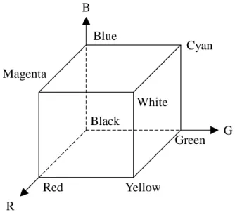
In the RGB model, each color appears in its primary spectral components of Red, Green, and Blue. This model is based on a Cartesian coordinate system, its color subspace of interest is the cube shown in Fig. 2-1. It is a hardware-oriented model, which is most commonly used for color monitors and a broad class of color video cameras. Therefore, processing images in the RGB color space directly is the fast method. However it is not natural for human’s perception. We can summarize by saying that RGB is ideal for image color generation, but its use for color description is much more limited.

G R B Red Yellow White Green Cyan Black Magenta Blue

Fig. 2-1 RGB color cube.

2.1.2 HSI Color Model

The HSI color model is composed of Hue, Saturation, and Intensity. It is referred to HSV color model using the term Value instead of Intensity. Intensity is the brightness value, Hue and Saturation encode the chromaticity values. The HSI is very important and attractive for image processing since it represents colors similar to which human eye senses.

Given an image in RGB color format, the H component of each RGB pixel is obtained using the equation [1]

360 > θ θ ≤ ⎧ = ⎨ ₋ ⎩ if B G H if B G ( 1 ) where

(

) (

)

(

) (

)

The saturation component is given by

(

)

(

)

Finally, the intensity component is given by

(

)

1 3

= + +

I R G B ( 4 )

Fig. 2-2 shows the HSI model based on color circles. The Hue component describes the color itself in the form of an angle between [0,360] degrees. 0 degree mean red, 120 means green 240 means blue. 60 degrees is yellow, 300 degrees is magenta. The Saturation component signals how much the color is polluted with white color. The range of the S component is [0,1]. The Intensity range is between [0,1] and 0 means black, 1 means white.

2.1.3 YUV and YIQ Color Model

In the YUV color model, Y represents the luminance of a color while I and Q represent the chromaticity of a color. The conversion of RGB to YUV is given by [2].

0.30 0.59 0.11 0.493*( ) 0.877 * ( ) = + + = − = − Y R G B U B Y V R Y ( 5 )

The YIQ is used in NTSC color TV broadcasting. The original meanings of these names came from combinations of analog signals – I for in-phase chrominance, and Q for quadrature chrominance. The conversion of RGB to YIQ is given by [2].

0.299 * 0.587 * 0.114* 0.596* 0.275* 0.321* 0.212* 0.523* 0.311* = + + = − − = − + Y R G B I R G B Q R G B ( 6 )

The luminance-chrominance color models (YIQ, YUV) are proven effective. Hence, they are also adopted in image compression standards such as JPEG and JPEG2000. The YUV color space is very similar to the YIQ color space and both were proposed to be used with the NTSC standard, but because the YUV do not best correspond to actual human perceptual color sensitivities. NTSC uses I and Q instead.

2.1.4 XYZ Color Model

0.607 * 0.174 * 0.200 * 0.299 * 0.587 * 0.114 * 0.000 * 0.066 * 1.116 * = + + = + + = + + X R G B Y R G B Z R G B ( 7 )

2.1.5 L*a*b* Color Model

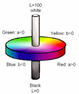
L*a*b* color model (also known as CIELAB) is a kind of visual uniform color system proposed by C.I.E. Its color model is shown in Fig. 2-3. The L* value represents luminance and ranges from 0 for black to 100. The maximum and minimum of value a* correspond to red and green, while b* ranges from yellow to blue.

Fig. 2-3 L*a*b* color model

1/ 3 1/ 3 1/ 3 1/ 3 1/ 3 * 116 16 * 500 * 200

with , , the values of the white point.

⎛ ⎞ = _{⎜ ⎟} − ⎝ ⎠ ⎡_{⎛ ⎞ ⎛ ⎞} ⎤ ⎢ ⎥ = _{⎜ ⎟} −_{⎜ ⎟} ⎢⎝ ⎠ ⎝ ⎠ ⎥ ⎣ ⎦ ⎡_{⎛ ⎞ ⎛ ⎞} ⎤ ⎢ ⎥ = _{⎜ ⎟} −_{⎜ ⎟} ⎢⎝ ⎠ ⎝ ⎠ ⎥ ⎣ ⎦ n n n n n n n n Y L Y X Y a X Y Y Z b Y Z X Y Z XYZ ( 8 )

2.1.6 Comparison of above Color Models

Above color models has been claimed by many research that they are the most suitable color model for some reasons. In Table2-1, we list the comparison [3] of these color models in the following five terms.

A. Is the color model device independent? B. Is the color model perceptual uniform? C. Is the color model linear?

D. Is the color model intuitive?

E. Is the color model robust against varying imaging conditions?

Table 2-1 Characteristics of each color models

A B C D E

RGB N N N N

Dependent on viewing direction, object geometry, direction of the illumination, intensity and color of the illumination.

HSI N N H:N Y H: Dependent on the color of the

S: N S: Dependent on highlights and a change in the color of the illumination

I:Y

I: Dependent on viewing direction, object geometry, direction of the illumination, intensity and color of the illumination. YUV

and YIQ

Y N Y N

Dependent on viewing direction, object geometry, highlights, direction of the illumination, intensity and color of the illumination.

XYZ Y N Y N

Dependent on viewing direction, object geometry, highlights, direction of the illumination, intensity and color of the illumination.

L*a*b* Y Y N N

Dependent on viewing direction, object geometry, highlights, direction of the illumination, intensity and color of the illumination.

2.2 Color Features

The most frequently cited visual features for image retrieval are color, texture, and shape. Among them, the color feature is most commonly used. It is robust to complex background and independent of image size and orientation. In this section, we will introduce two color features, color histogram, and color moment.

2.2.1 Color Histogram

Color Histogram is the most popular feature that is used in image retrieval. It is a global image feature. The advantages of color histogram are simple operation, invariant to translation, rotation, and scales of images.

A color histogram of an image counts the number of pixels with a given pixel value in red, green, and blue (RGB). To save storage and smooth out differences in similar but unequal images, the histogram is defined coarsely, with bins quantized to 8 bits, with 3 bits for each of red and green and 2 for blue.

2.2.2 Color Moment Primitives

The color distribution of an image can be characterized by color moments. Primitives of color moments [6] of an image can be viewed as a partial image feature. This feature contains local and global information of an image such that partly similar images will be retrieved.

The first color moment of the i -th color component (i=1,2,3) is defined by

1 , 1 1 N i i j j M p N = =

∑

where p is the color value of the i-th color component of the j-th image pixel and N is the _{i j,} total number of pixels in the image. The h-th image moment, h=2,3,…, of the i-th color component is then defined as

(

)

∑

Take the first H moments of each color component in an image s to form a feature vector, CT, which is defined as 1 2 1 2 1 2 1 1 1 1 1 1 2 2 2 2 2 2 1 2 3 3 3 3 3 3 [ , ,..., ] [ , ,..., , , ,..., , , ,..., ] Z H H H CT ct ct ct M M M M M M M M M α α α α α α α α α = = ( 11 )

where Z=H*3 and α α α₁, ₂, ₃ are the weights for Y, I, Q.

Based on the above definition, an image is first divided into X non-overlapping blocks.

For each block a, its h-th color moment of the i-th color component is defined byM_{a i}h_. . Then, the feature vector, CB , of block a is represented as _a

,1 ,2 , 1 2 1 2 1 .1 1 .1 1 .1 2 .2 2 .2 2 .2 1 2 3 .3 3 .3 3 .3 [ , ,..., ] [ , ,..., , , ,..., , , ,..., ] a a a a Z H H a a a a a a H a a a CB cb cb cb M M M M M M M M M α α α α α α α α α = = ( 12 )

From the above definition we can obtain X feature vectors. To speed up the image

retrieval, we will find some representative feature vectors to stand for these feature vectors. To reach this aim, a progressive constructive clustering algorithm [7] is used to classify all

a

CB s into several clusters and the central vector of each cluster is regarded as a representative vector and called the primitive of the image. The central vector, PC , of the k-th cluster is _k defined by .1 .2 . .1 .2 . 1 1 1 1 [ , ,..., ] , ,..., k k k k k k k k Z n n n n k k k k j j j j Z j j j j k k k k PC pc pc pc CB cb cb cb n n n n = = = = = ⎡ ⎤ ⎢ ⎥ ⎢ ⎥ = = ⎢ ⎥ ⎢ ⎥ ⎣ ⎦

∑

∑

∑

∑

where CBkj, 1, 2,...,j= nk,belongs to the k-th cluster and n is the size of the k-th cluster. k

2.3 Morphological Operator

are useful in the representation and description of region shape, such as boundaries, skeletons, texture, and the convex hull. Mathematical morphology is a set-theoretic method. Sets in mathematical morphology represent the shapes of objects in an image. The operations of mathematical morphology were originally defined as set operations and shown to be useful for image processing.

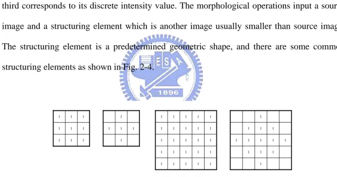
In general, morphological approach is based upon binary images. In binary images, each pixel can be viewed as an element in Z . Gray-scale digital images can be represented as 2 sets whose components are in Z , two components are the coordinates of a pixel, and the 3 third corresponds to its discrete intensity value. The morphological operations input a source image and a structuring element which is another image usually smaller than source image. The structuring element is a predetermined geometric shape, and there are some common structuring elements as shown in Fig. 2-4.

1 1 1 1 1 1 1 1 1 1 1 1 1 1 1 1 1 1 1 1 1 1 1 1 1 1 1 1 1 1 1 1 1 1 1 1 1 1 1 1 1 1 1 1 1 1 1 1 1 1 1 1

Fig. 2-4 Examples of structuring elements.

Here, we will discuss morphological operators in binary images [1, 7]. Given a source image A and a structuring element B inZ , with components a and b respectively. And 2 φ denotes the empty set.

The Translation of A by the point x inZ , denoted2 A_xv, is defined by

{

}

x

Av = av v+x ∀ ∈av A = +A xv ( 14 )

where the plus sign refers to vector addition.

And the Reflection of B, denoted Bˆ , is defined as

{

}

B= −b bv v∈B ( 15 )

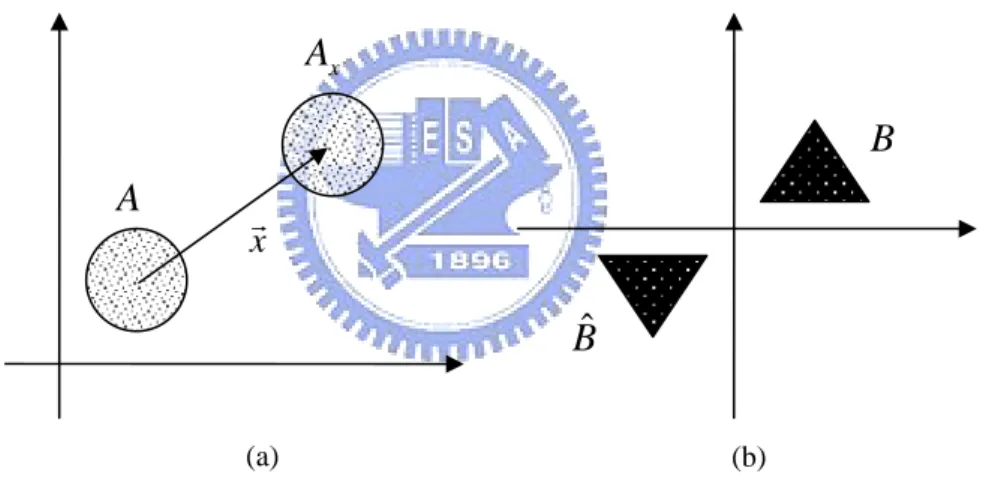
The examples of Translation and Reflection are shown in Fig. 2-5.

Fig. 2-5 Examples of (a) Translation and (b) Reflection.

2.3.2 Dilation, Erosion, Opening ,and Closing of Binary Images

We introduce two of the fundamental morphology operations：Dilation and Erosion used in binary images, and two operators：Closing and opening that extended from Dilation and Erosion.

The Dilation of A by B, denotedD

( )

xr x A A B Bˆ (a) (b)

( )

{

}

B

D A = ⊕ =A B x Bv + ∩ ≠xv A φ ( 16 )

where B is the structuring element.

And the Erosion of A by B, denotedEB

( )

( )

{

}

B

E A =A B0 = x Bv + ⊂xv A ( 17 )

Fig. 2-6(c) and (d) are examples of Dilation and Erosion. The dilation of A by B is the set of all xv displacements such that Bˆ and A overlap by at least one nonzero element. The erosion of A by B is the set of all points xv such that B translated by xv is contained in A. The Closing of set A by structuring element B, denotedC_B

( )

( )

(

( )

)

(

)

B B B

C A = • =A B E D A = A⊕ 0B B ( 18 )

And the Opening of set A by structuring element B, denoted O_B

( )

( )

(

( )

)

(

)

B B B

O A = A B_o =D E A = A B0 ⊕B ( 19 )

The examples of closing and opening are shown in Fig. 2-6(e) and (f). The closing of A by B is simply the dilation of A by B, followed by the erosion of the result by Bˆ . The opening of A by B is simply the erosion of A by B, followed by the dilation of the result by Bˆ .

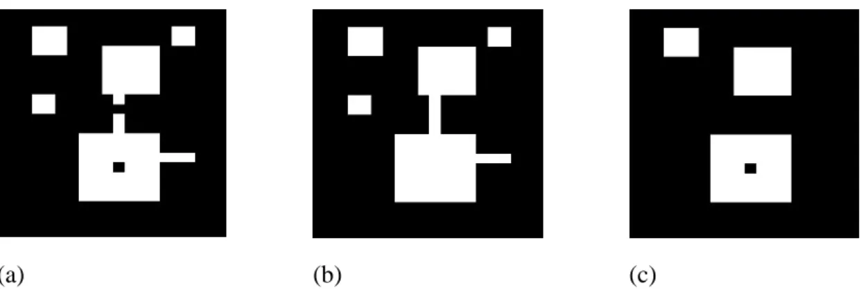
Another examples of closing and opening are shown in Fig. 2-7(b) and (c). From the figure, closing will connect thin lines and fill small holes and opening will leave objects larger than structuring element and subtract small thin lines.

(a). Set A (b). Structuring element B

(c). Dilation (d). Erosion

(e). Closing (f). Opening

Fig. 2-6 (a). Set A. (b) Structuring element B. (c). The Dilation of A by B. (d). The Erosion of A by B. (e). The Closing of A by B. (f). The Opening of A by B.

(a) (b) (c)

Fig. 2-7 (a) original image (b)(c) closing and opening with 3*3 structuring element, respectively.

In this section, we extend to gray-level images the basic operations of dilation, and erosion. Throughout the discussions that follow, we deal with digital image functions of the forms f x y and ( , )( , ) b x y , where ( , )f x y is the gray-scale image and ( , )b x y is a structuring element.

Gray-Scale dilation of f by b, denoted by f ⊕ , is define as： b

(f ⊕b s t)( , )=max{ (f s−x t, −y)+b x y( , ) (s−x), (t− ∈y) D_f; ( , )x y ∈D_b} ( 20 )

where D_f and D are the domain of _b f and b , respectively. As before, b is the structuring element of the morphological process but note that b is now a function rather than a set. Because dilation is based on choosing the maximum value of f + b in a neighborhood defined by the shape of the structuring element, the general effect of performing dilation on a gray-scale image is two-fold: (1) if all the values of the structuring element are positive, the output image tends to be brighter than the input; and (2) dark details either are reduced or eliminated, depending on how their values and shapes relate to the structuring element used for dilation. As illustrated in Fig 2-8 (b).

Gray-scale erosion of f by b, denoted by f0 , is define as： b

(f0b s t)( , )=min{ (f s+x t, +y)−b x y( , ) (s+x), (t+y)∈Df; ( , )x y ∈Db} ( 21 )

where D_f and D are the domain of _b f and b . Because erosion is based on choosing the minimum values of f − in a neighborhood defined by the shape of the structuring element, b the general effect of performing erosion on a gray-scale image is two-fold: (1) if all the values of the structuring element are positive, the output image tends to be darker than the input; and

(2) bright details are reduced or eliminated, depending on the used structuring element. As illustrated in Fig 2-8 (c).

(a) (b) (c)

Fig. 2-8 (a) The original of Lena image (b) Dilation of Lena image (c) Erosion of Lena image.

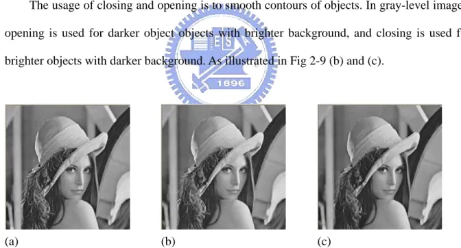
The usage of closing and opening is to smooth contours of objects. In gray-level images, opening is used for darker object objects with brighter background, and closing is used for brighter objects with darker background. As illustrated in Fig 2-9 (b) and (c).

(a) (b) (c)

Fig. 2-9 (a) The original of Lena image (b) Closing of Lena image (c) Opening of Lena image.

2.3.4 Morphological Gradient

( )

( ) (

) (

)

( )

(

)

( )

(

)

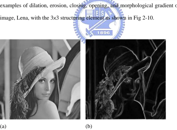
The morphological gradient highlights sharp gray-scale transitions in the source image. In other words, morphological can extract the boundary of an object. However, the morphological gradient is sensitive to the shape of the chosen structuring element. Here are examples of dilation, erosion, closing, opening, and morphological gradient of the gray-scale image, Lena, with the 3×3 structuring element as shown in Fig 2-10.

(a) (b)

Fig. 2-10 (a) The original of Lena image (b) Morphological gradient of Lena image

Granulometries were introduced first by G. Matheron [8], and have been proven to be very useful in image analysis, finding application in image tasks such as texture classification, pattern analysis, and image segmentation. A granulometry can simply be defined as series of morphological openings with structuring elements of increasing sizes. The granulometric function maps each structuring element size to the number of image pixels removed during the opening operation with the corresponding structuring element. It is easy to extend the binary granulometry into grayscale form by replacing the binary opening with a grayscale opening.

There are three kinds of granulometric function [9]:

1 Number of particles of ( ) k S f γ . 2 Surface area of ( ) k S f

γ , often called size distribution. This measure is typically chosen to be the area (number of ON pixels) in the binary case, and the volume (sum of all pixel values) in the grayscale case.

3 Loss of surface area between ( )

k S f γ and 1( ) k S f

γ ₋ , called the granulometric curve, or

pattern spectrum.

where γ is the binary morphological opening, f represents the original image, and

, 1, 2,...

k

S k= , is a sequence of opening structuring elements of increasing size.

2.3.6 Morphological Primitives

This feature is proposed by J-S Wu [10]. Before the morphological operation, first we transform RGB color model into YIQ model for the sack of human perception. Then we

value of the down-sampled image located at

( )

( )

[

]

where b is a structuring element, Db(Yx,y),Db(Ix,y),Db(Qx,y) are the dilation of Y, I, Q color channels respectively; Eb(Yx,y),Eb(Ix,y),Eb(Qx,y) are the erosion of Y, I, Q color channels respectively; Gb(Yx,y),Gb(Ix,y),Gb(Qx,y) are the morphological gradient of Y, I, Q color channels respectively.

From the definition above, we get both the color and shape information of a pixel within the filter. We use large morphological gradient value to identify an edge pixel, and a small one to a pixel on a flat region. Then we get the color information in the neighborhood of the edge pixels. Therefore, two pixels with the same color value might not have the same context.

After morphological context extraction, there will be many similar contexts. So we use the following algorithm to cluster these contexts to small number of contexts which are more representative.

1. Initially, we extract the first pixel’s context, and then this context is viewed as the center of the first cluster.

currently existing clusters. If the nearest distance is smaller than a threshold, T , then d

assign this context to the nearest cluster and update MP_nearest. Otherwise, construct a new cluster that the cluster center is Cx,y

3. Repeat .step2 until all pixels are processed.

In the above algorithm, MPnearest is defined by

[

]

∑

∑

∑

∑

where C_xk_,y, j=1,...,n_k, is the context located at (x,y) and belongs the k-th context cluster. Moreover, the Euclidean distance between C_x,y and MP is defined as follows: _k

(

)

∑

2.4 Distance Functions for Similarity Measure

For measuring perceptual similarity between images, many distance functions have been used. Here we will introduce Minkowski-like metrics [4] and Dynamic Partial Function [5].

Histogram intersection is the standard measure used for color histograms. First, a color histogram H is generated for each image i in the database. Next, each histogram is _i normalized, so that its sum equals unity. After this step, it effectively removes the size of image. The histogram is then stored in the database. For any selected model image, its histogram H is intersected with all database image histograms _m H , according to the _i equation 1 intersection min( , ) = =

∑

where j denotes histogram bin j , with each histogram having n bins. The closer

intersection value is to 1, the better the image match.

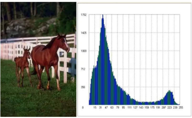
Although, it is fast to compute the histogram, the intersection value is sensitive to color quantization. And two different images may have similar color histograms as shown in Fig. 2-11. Therefore, only use the color histogram as color feature of image is not enough for image retrieval.

Fig. 2-11 Two different images with similar color histograms.

2.4.2 Primitive Similarity

First, we provide several definitions. The k -th primitive of a query image q is

represented as: .1 .2 . [ , ,..., ] , where 1, 2 ,..., , q q q q k k k k Z PC = pc pc pc k= m ( 29 )

and m is the number of primitives in the query image. Theλ -th primitive of a matching image s is denoted as .1 .2 . [ , ,..., ] s s s s Z PC_λ = pc_λ pc_λ pc_λ ( 30 )

The distance between PC and _kq PC_λs is defined as follows:

(

)

∑

(

)

, ,

.

_ kq s min _ kq s

D PC = λ D PC λ ( 32 )

The distance between the query image q and the matching image s is defined by

, , k=1 _ _ m q s q q s k k D PC =

∑

wheren is the size of the k-th cluster. The similarity measure between q and s is defined as _kq

, , 1 _ q s q s Sim D PC = ( 34 )

Note that the largerSimq s, a matching image has, the more similar it is to the query image.

2.4.3 Minkowski-Like Metrics

Each image can be represented by a p-dimensional feature vector ( ,x x_{1 2},...,x_p),

where each dimension represents an extracted feature. Δdi= xi−yi , i=1,2, . . .,p is defined

as the feature distance in feature channel i . Minkowski-like distance functions are commonly used to measure similarity. The distance between any two images, X and Y, is defined as

1/ p 1 ( , ) = ⎛ ⎞ =_⎜ Δ _⎟ ⎝

∑

When r=1, above distance is the City-block or L1 distance. When we set r =2, it is the Euclidean or L2 distance. And, when r is a fraction, it defines a fractional function.

To disagree with Minkowski-like metric, DPF does not consider all features for similarity measurement. If we define the similar data set

1 2

The smallest ' of ( , ,..., )

Δ =_m m d sΔ _i Δ Δd d Δd_p ( 36 )

then the dynamic partial distance between two image X and Y, is defined as

1/ ( , ) Δ ∈Δ ⎛ ⎞ =_⎜ Δ _⎟ ⎝

∑

where m and r are tunable parameters. When m= p , DPF degenerates to a Minkowski-like metric. When m< p , it counts the smallest m feature distances between two images.

Studies have shown [5] that the Minkowski approach does not model human perception. The performance of DPF has been shown [5] to be superior to that of widely-used distance functions, For instance, for a recall of 80 percent, the retrieval precision of DPF is shown to be 84 percent for the test data set used.

2.4.5 The DPF Enhancement 2.4.5.1 Thresholding Method

Here, we select the features that have a difference smaller than θ belong to the similar feature set A . The Thresholding distance of image pair (X,Y) is then defined as _θ

1/ 1 ( , ) θ θ Δ ∈ ⎛ ⎞ ⎜ ⎟ = Δ ⎜ ⎟ ⎝ _n

∑

The main idea of Sampling-DPF is to try different m settings simultaneously and to guess that some of the sampling points can be near the optimal m. Suppose we sample N

settings of m, denoted as m , 1,...,_n n= N . At each sampling m , a ranking list, denoted as _n ( ,Φ )

n

R X , is generated. Finally, the sampling method obtains N ranking lists and produces

the final ranking, denoted as R_r( ,Φ X . )

Two methods are suggested, one is using the smallest rank as the final rank (SR). The other is using the average distance (or rank) as the final distance (AR). The AR distance is defined as 1/ 1 1 ( , ) = Δ ∈Δ ⎛ ⎞ = _⎜ Δ _⎟ ⎝ ⎠

∑ ∑

For the Sampling-Thresholding method, its AR distance is defined as

1/ 1 1 1 ( , ) θ θ = Δ ∈ ⎛ ⎞ ⎜ ⎟ = Δ ⎜ ⎟ ⎝ ⎠

∑

∑

The Weighting method can be used with Sampling-DPF, Sampling-Thresholding, or other methods. It considers that different types of features can have different degrees of importance for measuring similarity. Let ω_i denote the weight of the i th similar feature. In the Weighted-Sampling-DPF method, the distance of image pair (X,Y) is defined as

1/ 1 1 ( , ) ω = Δ ∈Δ ⎛ ⎞ = _⎜ Δ _⎟ ⎝ ⎠

∑ ∑

and in the Weighted-Sampling-Thresholding method, it is defined as 1/ 1 1 1 ( , ) θ θ ω = Δ ∈ ⎛ ⎞ ⎜ ⎟ = Δ ⎜ ⎟ ⎝ ⎠

∑

∑

Chapter 3

The Proposed Method

Overview of our retrieval system is described in section 3.1. In section 3.2, we will introduce a new feature, granulometric histogram, which represents the size distribution of an image. Its similarity is described in section 3.3.1. We also introduce the smallest DPF to be the similarity of Morphological Primitive and describe it in section 3.3.2.

3.1 Overview

Fig-3.1 shows the architecture of our retrieval system. Within it, processing and similarity measure are the key components. There are many processing methods for the purpose of image retrieval. In this thesis, we employe morphological primitive extraction, color moment primitive extraction, morphological granulometric distribution, and morphological granulometric histogram. We plot them in Fig-3.2.

Images in image database Indexing Retrieval Feature Database processing Retrieval result Similarity measure Query image processing Images in image database

Indexing Retrieval Feature Database processing Retrieval result Similarity measure Query image processing

Fig. 3-1 Architecture of our retrieval system.

YIQ Color Transform Morphological Primitives extraction processing YIQ Color Transform Morphological Primitives extraction processing (a) YIQ Color Transform Color Moment Primitives extraction processing YIQ Color Transform Color Moment Primitives extraction processing (b) YIQ Color Transform Morphological Granulometric Distribution processing YIQ Color Transform Morphological Granulometric Distribution processing (c) RGB Color Transform Morphological Granulometric Histogram processing RGB Color Transform Morphological Granulometric Histogram processing (d) YIQ Color Transform Morphological Granulometric Histogram processing YIQ Color Transform Morphological Granulometric Histogram processing (e)

3.2 Morphological Granulometry

3.2.1 Distribution of Morphological Granulometry

Before applying morphological granulometry, we transform the down-sampled image

from RGB to YIQ color model. Assume Cx,y =

(

)

( )

{

}

with increasing sizes. According to section 2.3.5, we have chosen the pattern spectrum as the granulometry function.

First, we do a series of morphological openings, denoted O (Y),O (I),O (Q)

i i

i b b

b , to each

component of YIQ color space with structuring element bi,i=1,...,L. Therefore, we obtain

L

M =3* openings for a single image.

Second, we compute the distribution of morphological granulometry as follows:

} ) ( ) ( ) ( ) ( ) ( ) ( { ) ; ; 1 int for( 1 1 1 Q O Q O DQ I O I O DI Y O Y O DY i L i i i i i i i i b b i b b i b b i − = − = − = + + <= = − − − Here, )( 0 Y

} in pixles of number / in pixles of number / in pixles of number / } ; ) 0 ) , ( ( if ; ) 0 ) , ( ( if ; ) 0 ) , ( ( if { ) , ( all for ; 0 ; 0 ; 0 { ) ; ; 1 int for( Q GQ I GI Y GY GQ y x DQ GI y x DI GY y x DY y x GQ GI GY i L i i i i i i i i i i i i i i = = = + + > + + > + + > = = = + + <= =

Then, (GY1,GY2,...,GYL), (GI1,GI2,...,GIL), and (GQ1,GQ2,...,GQL) are size

distributions of Y , I , and Q , respectively.

3.2.2 Primitives of Granulometric Distribution

As morphological primitive mentioned in 2.3.6, we first transform RGB color model into

YIQ model, then we down-sample each image. Let f(x,y)=

(

)

value of the down-sampled image located at

( )

( )

[

]

) 1 ( *

3 L

Z = + . If Z =6 . Yx,y,Ix,y,Q are the pixel value of Y, I, Q color channels respectively; )Ob(Yx,y),Ob(Ix,y),Ob(Qx,y are the openings of Y, I, Q color channels

respectively. Consequently, 6, 5 , 4 ,y, xy, xy x c c

c represent the pattern spectrum.

3.2.3 Histogram of Morphological Granulometry

The granulometric histograms are obtained by the following four steps.

First, we down-sampled the target image to remove the noise and reduce the computation

time. Suppose Cx,y =

(

)

( )

down-sampled image.

Second, letB=

{

}

do a series of morphological openings, denoted O (R),O (G),O (B)

i i

i b b

b , to each component of

color space with structuring element b_i,i =1,...,L. Therefore, we obtain M =3*L openings for a single image.

Third, we count the histogram Hj, j=1,...,M of each opening, says the granulometric

histograms. H₁,H₂,...,H_L are histograms of O R j L

j b ( ), =1,..., , respectively, L L L H H H ₊₁, ₊₂,..., _2* are histograms of O G j L j b ( ), =1,..., , respectively, L L L H H H_{2* +1}, _{2* +2},..., _3* are histograms of O B j L j b ( ), =1,..., , respectively.

Fourth, we normalize the histogram. So Hj =Hj/num , 1,...,j= M where 255 0 i j i num H =

=

∑

Morphological opening or closing could enhance, suppress or smooth some areas. Opening operation of a particular size of structuring element has the most effect on regions of the input image that contain particles of that size.

In RGB color space, it is easy to treat similar colors as different colors and then similar objects become different objects. Opening of different image may be similar under RGB color space.

Take Fig.3-3 for example. The space between trunks of trees and space separated by legs of horses in Fig.3-3(a) are then becoming blocks of colors after opening. The chinks in the leaves, color changing in the trees, and the stripes of the bus are causing blockings after opening. We may see those blocks in Fig.3-4 and Fig.3-5. These phenomenon leads to false retrieval results.

(a) (b)

(a) R component (b) opening of (a) with b1 (c) opening of (a) with b2

(d) G component (e) opening of (d) with b₁ (f) opening of (d) with b₂

(g) B component (h) opening of (g) with b1 (i) opening of (h) with b2

Fig. 3-4 Openings of .Fig.3-3(a).

(a) R component (b) opening of (a) with b₁ (c) opening of (a) with b₂

(g) B component (h) opening of (g) with b1 (i) opening of (h) with b2

Fig. 3-5 Openings of Fig.3-3(b).

We improve this problem by changing RGB into YIQ color model for the sake of human perception and linear transform. In this color space, the false segmentation of one object with some similar colors can be avoided.

Use the same images mentioned above for example. The openings of Fig.3-3 under YIQ are listed in Fig-3.6 and Fig-3.7. Only Y component, the luminance part has similar blocking effect as which under RGB color model. We can see the blur shape of horse and bus with light gray in I and Q components.

Therefore, the granulometry histogram gives more information about size of objects than luminance information of objects. If the size of objects in query image and that of matching images are closed, they will be retrieved as similar images. Since the histogram has been normalized, it is independent of image size. It depends only if the ratio of object size and image size are very different. That is, this histogram says dissimilar when the same object in different images has large variations in ratio of object size and image size, or says similar when different objects in different images have the same ratio of object size and image size.

(a) Y component (b) opening of (a) with b1 _{(c) opening of (a) with} 2

b

(d) I component (e) opening of (d) with b₁ (f) opening of (d) with b₂

(g) Q component (h) opening of (g) with b1 (i) opening of (h) with b2

Fig. 3-6 Openings of .Fig.3-3(a) under YIQ.

(a) Y component (b) opening of (a) with b1 (c) opening of (a) with b2

(g) Q component (h) opening of (g) with b1 (i) opening of (h) with b2

Fig. 3-7 Openings of .Fig.3-3(b) under YIQ.

3.3 Similarity

3.3.1 Similarity for Morphological Granulometry

We use absolute difference as the similarity measure for granulometric distribution. Therefore, similarity of granulometric distribution equals the sum of M absolute difference between target and matching images.

Besides, we choose intersection as the similarity measure for granulometric histogram. Hence, similarity of granulometric histogram equals M minus the sum of M histogram intersection.

3.3.2 DPF for Primitives

Here, we propose a new similarity measure for primitives, the DPF. The distance between two N-tuple primitive vectors is the sum of the smallest βbins where β < . N This idea comes from some problem of thresholding method. It is difficult to set a fixed threshold that is suitable for every image. And once a threshold T has been set, it is possible that non of the distance within the bins of the feature vectors is less than T . To make sure at least one feature bin has been considered, we choose some smallest bin distance as the

Follow the definitions of primitive similarity in section 2.4.2. We only update the

distance between PC and _kq PC_λs into the following equation:

∑

where d is the smallest j th element of j

{

}

q s k i i

pc −pc_λ i= N . The rest are the same as

Chapter 4

Experimental Results

In this chapter, we will present some experimental results obtained by applying the proposed methods. We also compare the results with color histogram, morphological primitives [10] and color moment primitives [6].

4.1 Experimental environment

The 1000 test images are selected from Corel’s database, and classified to 10 types of models, beach, buildings, buses, dinosaurs, elephants, flowers, horses, underwater worlds, and foods. Each type contains 100 images. Fig. 4-1 show some examples of each type from the database. The image size is either 384*256 or 256*384 pixels.

Images have similar object size in each of type 1, 4, 5, 6, 7, 8, and 9, respectively. Only type 1, 5, 9 have clean background. We define that an image has a clean background for there isn’t too many variant colors or objects inside and with a large area of some similar colors. Objects in images of type 2, 3, 10 are very complicated. But every image has blue sky and ocean in type 2, has buildings in type 3, and has plates in type 10. Some images in type 3 also have blue sky.

(a) Type 1 (b) Type 2 (c) Type 3 (d) Type 4 (e) Type 5

(f) Type 6 (g) Type 7 (h) Type 8 (i) Type 9 (j) Type 10 Fig. 4-1 Examples of the image database.

The proposed methods are implemented on PC with Pentium4 2.8GHz, RAM 1G.. The operating system is Microsoft Windows XP SP2. The program was developed in the C++ language and compiled under Borland C++ Builder version 6.0. Our feature database is built in MySQL for the sake of its combination with PHP in the network.

The first experiment compares the results of morphological primitives (MP) using smallest DPF and original primitive similarity measure. The second experiment shows the results of morphological granulometric distribution (GD) and its primitives (GDP). The third experiment demonstrates the results of the granulometry histogram under RGB (GHrgb) and YIQ (GHyiq) color model. The fourth experiment compares granulometry histogram, granulometric distribution, primitives of granulometric distribution, morphological primitives

(MP), primitives of color moments (CMP), and color histogram (CH). And finally, we introduce the fifth experiment to verify the robustness of our image retrieval system.

4.2 Experimental results

We use precision and recall to measure our image retrieval system. The definitions of them are described in the following text. Assume that R is the number of retrieved relevant images, T is the total number of relevant images and K is the number of retrieved images. Then, K R = Precision ( 45 ) T R = Recall ( 46 ) 4.2.1 Morphological Primitives

Morphological Primitive using smallest-8 DPF has improved the precision of all types in image database except type5 dinosaur. In Fig.4-2, MP means MP using similarity in section 2.4.2, MP8 and MP7 means MP using the smallest-8 and smallest-7 DPF, respectively. We only show the results of three types (model, dinosaur, and horse) in Fig.4-2.

In type1 model, the curve of MP7 is slightly lower than the other two curves when recall is less than 75, but larger than the other two when recall is larger than 75. When retrieve for the top 97, precisions of MP, MP8, and MP7 are 38%, 50%, 70%, respectively. Precision of MP7 for top 97 increases 32% to compare with MP. In type5 dinosaur, the curve of MP8 and MP7 are both lower than that of MP.

The consistency of regular object size and clean background upgrades the precision-recall curve. Although type1 and type5 both have clean background, models have two object sizes while dinosaurs have only one. There is space for improvement in type1 not in type5. That’s why two types with similar options are not both upgraded when using DPF.

Type1: Model 20% 30% 40% 50% 60% 70% 80% 90% 100% 1 10 20 30 40 50 60 70 80 90 100 Recall P re cis ion _MP MP8 MP7 (a) Type8: Horse 10% 20% 30% 40% 50% 60% 70% 80% 90% 100% 1 10 20 30 40 50 60 70 80 90 100 Recall P re cis ion _MP MP8 MP7 (b)

Type5: Dinosaur 10% 20% 30% 40% 50% 60% 70% 80% 90% 100% 1 10 20 30 40 50 60 70 80 90 100 Recall P reci si on _MP MP8 MP7 (c)

Fig. 4-2 The Precision-Recall curves when using morphological primitives. (a) The results of Type1 (b) The results of Type7 (c) The results of Type5.

4.2.2 Granulometric Distribution and its Primitives

We use five different numbers of sets of structuring elements to experiment on granulometric distribution. The precision-recall curves are very close with each other. Consequently, we choose the set of seven structuring elements to attain the average precision and take less computation time. Then, we try on its primitives with Z =6,9. On average, precisions of GDPs are better than those of GDs, but all lower than those of GHs (see next section). Precision curves in Fig. 4-3 show that GH has the best performance.

20% 30% 40% 50% 60% 70% 80% 90% 100% 1 2 3 4 5 6 7 8 9 10 Type Number Pr ec is io n GH1rgb GH7rgb GH1yiq GD7 GDP6 GDP9

Fig. 4-3 The precision comparison for each type of image database among the proposed methods, granulometric histogram, granulometric distribution, and primitives of granulometric distribution (R=20).

4.2.3 Granulometric Histogram

We suppose M =1,2,...,7 for GH under RGB, and M =1,2,3 for GH under YIQ. In Fig. 4-4, GHk, k =1,2,...,7 means GH under RGB with M =k, and GHyiqk, k =1,2,3

means GH under YIQ with M =k.

From the results in Fig. 4-4, we may conclude that it is more suitable to take GH under YIQ as an object size feature than GH under RGB in most cases. Precision-recall curves of images with variant object size like type2 beach and type 9 under water will be degenerated. The sizes of two types, flowers and elephants, are very close. Therefore, the mismatching of these two type images is caused. The first type models is a little bit degenerated for the reason that images of models have not unique but two major sizes. The rest of types are all superior to those under RGB.

Type1: Model 20% 30% 40% 50% 60% 70% 80% 90% 100% 1 10 20 30 40 50 60 70 80 90 100 Recall P recis io n GH1 GH2 GH3 GH4 GH5 GH6 GH7 GHyiq1 GHyiq2 GHyiq3 (a) Type5: Dinosaur 20% 30% 40% 50% 60% 70% 80% 90% 100% 1 10 20 30 40 50 60 70 80 90 100 Recall Pr ec is io n GH1 GH2 GH3 GH4 GH5 GH6 GH7 GHyiq1 GHyiq2 GHyiq3 (b) Type6: Elephant 10% 20% 30% 40% 50% 60% 70% 80% 90% 100% 1 10 20 30 40 50 60 70 80 90 100 Recall Pre ci si on GH1 GH2 GH3 GH4 GH5 GH6 GH7 GHyiq1 GHyiq2 GHyiq3

Type8: Horse 10% 20% 30% 40% 50% 60% 70% 80% 90% 100% 1 10 20 30 40 50 60 70 80 90 100 Recall Pr ec is io n GH1 GH2 GH3 GH4 GH5 GH6 GH7 GHyiq1 GHyiq2 GHyiq3 (d)

Fig. 4-4 Comparison of GH under RGB and YIQ.

4.2.4 Comparisons

To show the performance of the proposed methods, the retrieval results are compared with those using morphological primitives, color moment primitives, and color histogram. Fig. 4-5 shows the precision-recall curves of each type in image database using different method. And Fig. 4-6 list the precisions of each method whenR=20. Due to the factor of object size, GH is a good feature for type1, 5, 6, 7, and 9. It is only below CH but above all other methods for type 3 and 8. And those are lower than other methods for type 2, 4 and 10.

We may see more clearly by compute the difference of precisions between the proposed method GH and other methods which are listed in Table 4-1. The best improvement of GH when compared with MP, CMP, and CH is 47%, 38%, and 37%, respectively, and the worst degradation is 5%, 14%, and 17%, respectively.

Type1: Model 20% 30% 40% 50% 60% 70% 80% 90% 100% 1 10 20 30 40 50 60 70 80 90 100 Recall Pre ci si on GHyiq1 GHrgb1 GHrgb7 MP MP8 CMP CH ClosingH (a) Type4: Bus 10% 20% 30% 40% 50% 60% 70% 80% 90% 100% 1 10 20 30 40 50 60 70 80 90 100 Recall Pre ci si on GHyiq1 GHrgb1 GHrgb7 MP MP8 CMP CH (b) Type5: Dinosaur 20% 30% 40% 50% 60% 70% 80% 90% 100% 1 10 20 30 40 50 60 70 80 90 100 Recall Pre ci si on GHyiq1 GHrgb1 GHrgb7 MP MP8 CMP CH

(c) Type8: Horse 10% 20% 30% 40% 50% 60% 70% 80% 90% 100% 1 10 20 30 40 50 60 70 80 90 100 Recall Pre ci si on GHyiq1 GHrgb1 GHrgb7 MP MP8 CMP CH (d)

Type9: Under water

10% 20% 30% 40% 50% 60% 70% 80% 90% 100% 1 10 20 30 40 50 60 70 80 90 100 Recall Pre ci si on GHyiq1 GHrgb1 GHrgb7 MP MP8 CMP CH (e)

20% 30% 40% 50% 60% 70% 80% 90% 100% 1 2 3 4 5 6 7 8 9 10 Type Number Pre ci si on GHyiq1 GHrgb1 GHrgb7 MP MP8 CMP CH

Fig. 4-6 The precision comparison for each type of image database among the proposed methods and other methods (R=20).

Table 4-1 Differences of precisions between proposed method GH and other methods (MP9, CMP, and CH).

MP9 CMP CH Type

max min max min max min

1 47% -2% 25% -3% 37% -2% 2 11% 0% 22% -1% 3% -2% 3 15% 0% 16% 0% 0% -11% 4 11% -5% 7% -11% 1% -3% 5 4% -3% 37% 0% 14% 0% 6 28% 0% 29% 0% 6% -6% 7 36% 0% 38% 0% 18% 0% 8 27% 0% 21% 0% 0% -6% 9 18% 0% 11% -13% 24% -2% 10 9% 0% 2% -14% 0% -17%

4.2.5 Example of Retrieval Results

We give an example of a flower image by retrieve the top relevant 20 images with methods mentioned above and show the results in Fig. 4-7. Precisions of CH, CMP, GH with YIQ, GH with RGB, MP7, MP8, and MP9 are 95%, 90%, 95%, 100%, 95%, 100%, and 90%,

(a) Color Histogram

(c) GH under YIQ with 1 structuring element

(e) Morphological Primitives with smallest-7 DPF

(g) Morphological Primitives

Fig. 4-7 Image retrieval using (a) Color Histogram (b) Color Moment Primitives (c) GH under YIQ with 1 structuring element (d) GH under RGB with 1 structuring element (e) Morphological Primitives with smallest-7 DPF (f) Morphological Primitives with smallest-8 DPF (g) Morphological Primitives for the top relevant 20 images.

4.2.6 Processsing Time

In Fig. 4-8, we show the average feature extraction time and average similarity measure time of methods discussed above. Our method takes less feature extraction time than MP and CMP, but almost three times of search time of CH since GH does intersection of three granulometric histogram.

Feature Extraction Time 0 0.01 0.02 0.03 0.04 0.05 0.06 0.07 0.08 CH CMP MP GH se conds (a) Search Time 0 1 2 3 4 5 CH CMP MP GH S eco nd s (b) Processing Time 0 1 2 3 4 5 CH CMP MP GH se co nds (c)