使用波茲曼模型方程式模擬自由分子流到近連續流的正方形空穴流場

國 立 交 通 大 學

機械工程學系 

碩士論文 

 

使用波茲曼模型方程式模擬自由分子流到近連續流的正方

形空穴流場 

 

 

Simulation of Square Driven Cavity Flows from 

Free‐Molecular to Near‐Continnum Regime Using Model 

Boltzmann Equation 

 

研究生：盧勁全 

指導教授：吳宗信  博士 

使用波茲曼模型方程式模擬自由分子流到近連續流的正方形空穴流場

Simulation of Square Driven Cavity Flows from Free-Molecular to

Near-Continnum Regime Using Model Boltzmann Equation

研 究 生：盧勁全 Student: Chin-Chuan Hung

指導教授：吳宗信 博士 Advisor: Dr. Jong-Shinn Wu

國立交通大學

機械工程學系

碩 士 論 文

A Thesis

Submitted to Institute of Mechanical Engineering

College of Engineering

National Chiao Tung University

in partial Fulfillment of the Requirements

for the Degree of

Master of Science

in

Mechanical Engineering

July 2007

Hsinchu, Taiwan

中華民國九十六年七月

致謝

誠蒙指導教授吳宗信老師的指導與督促，使得本文得以順利完成。在研究及做學問方 面，經老師的提攜與指點，讓我能順利的踏入研究的領域並且不斷地茁壯。此外老師對於台 灣本土精神及文化上的努力更是令我印象深刻。同時也感謝口試委員黃俊誠老師、郭添全博 士、陳明志老師在口試過程中所提供的珍貴意見，使得本文得以更加完善。另外特別感謝黃 俊誠老師長期發展關於此篇論文中所用到的程式之辛勞，且不吝於付出時間與心力來教導我 於研究中所遭遇的問題，以及粲哥、凱文在研究上的啟發教導與協助，在此一併致謝。 需要感謝的人實在太多了，邵雲龍、曾坤璋、許國賢、陳育進、梁偉豪、陳百彥等已 畢業的學長，還有 APPL 實驗室的成員，李允民、周欣芸、李富利、洪捷粲、許哲維、鄭凱 文、胡孟樺、邱沅明、江明鴻學長姊們指導受益良多，洪維呈、謝昇汎、林宗漢、陳又寧、 王柏勝、林武伸、邱文山、黃昌彥同學，與你們共同努力挑燈夜戰的每一天是我日後最甘苦 與美好的回憶，正勤、士傑、志良、玟琪、丞志、政霖、育宗等學弟妹們協助，還有來自紐 西蘭的學者 Hadley M. Cave 外語能力的訓練，使我兩年中過的非常充實且溫馨。 特別感謝爸爸、媽媽、兩位弟弟，在生活與精神上的支持，令我得以專心研究並且無 憂無慮。最後謝謝老婆思穎的關懷與體諒，給我無比的鼓勵，順利完成本文。僅將這份成果 獻給你們。歡樂的時光總是過的特別的快，又到時間講掰掰。畢業之後同學們各奔東西，盼 望大家都能闖出美好的將來。 盧勁全 謹誌 九六年七月于風城

使用波茲曼模型方程式模擬自由分子流到近連續流的正方

形空穴流場

學生:盧勁全 指導教授:吳宗信 博士

國立交通大學機械工程學系

摘 要

上板瞬間抽動的空穴流場在計算流體力學上是ㄧ個很基準的問題，因為 它具有簡單的幾何結構並且在其角落上有差異性很大的奇異點。在流場模擬 上,時常使用它來驗證不同的數值方法。然而,過去的學習都著重在連續流場 上的研究。關於稀薄流場與近連續流流場的研究則是相當的稀少。因此本文 的動機是模擬空穴流場在稀薄區域上的應用。 本文內容是利用建構在有限差分法(finite-difference scheme),速度空間上 應用分立座標法(discrete ordinate method)的波茲曼模型方程式(MBE)來模 擬二維的上板瞬間啟動之四方形穴流從自由分子流到近連續流的流場。本文 中使用BGK model與Shakov model兩種模型來近似碰撞積分項。為了驗證波茲 曼模型方程式(MBE)的正確性,我們比較直接蒙地卡羅模擬法(DSMC)與波茲曼 模型方程式(MBE)在模擬穴流Kn=0.0033 與 Ma=2.0的結果。本文中空穴流場 的模擬範圍包含了Kn=10~0.0033 與 Ma=0.5~2的流場。

象與溫度跳動現象會更加明顯。在各種的Mach number下 (M=0.5, 0.9, 1.1, 2), 隨 著 Kn 的 變 小 , 渦 流 中 心 會 朝 著 右 上 方 移 動 , 但 是 當 M=0.5,Kn=0.0033 與 M=2,Kn=0.0033時渦流中心會改變成朝左下方移動。此外當Kn小於0.01時,在 主要渦流的兩側角落都會產生出次渦流。當Kn大於0.01時,除了M=2,Kn=10這 個情況下會在右下角落產生一個次渦流以外,其他的情況則不會產生次渦流。

Simulation of Square Driven Cavity Flows from Free-Molecular to

Near-Continnum Regime Using Model Boltzmann Equation

Student: C. C. Lu Advisor: Dr. J. S. Wu

Department of Mechanical Engineering

National Chiao-Tung University

Abstract

The driven cavity flow is one of the benchmark problems often used in computational fluid dynamics due to its simple geometry but highly singular points at the corners. It is often used to verify different numerical methods for fluid-flow simulation. However, past studies in this regard focused on flows in thc continuum regime. Very few researches have been done systematically in the rarefied or near-contiuum regime. Several applications require consideration of rarefaction, which motivates the present thesis to focus on simulation of driven cavity flows in this region.

This thesis reports the simulation of a two-dimensional top driven square cavity flows from free-molecular to near-continuum regime using a model Boltzmann equation (MBE) solver. The MBE was discretized using finite-difference scheme and discrete ordinate method for the configuration and velocity space, respectively. The collision integral was approximated by either the BGK or Shakov model. The MBE

simulation Monte Carlo method for a driven cavity flow at Kn=0.0033 and Ma=2.0. Simulation conditions include Knudsen number and speed of the top driven plate in the range of Kn=10-0.0033 and Ma=0.5-2, respectively.

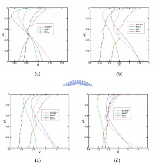
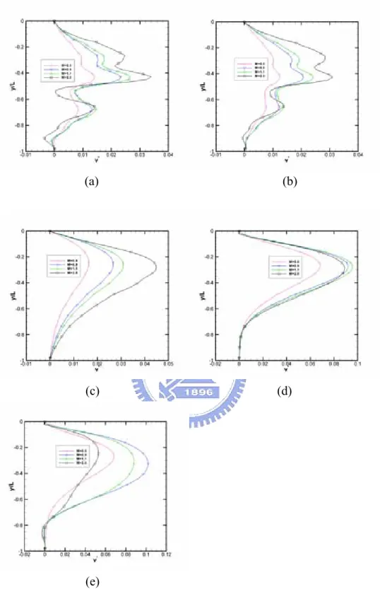
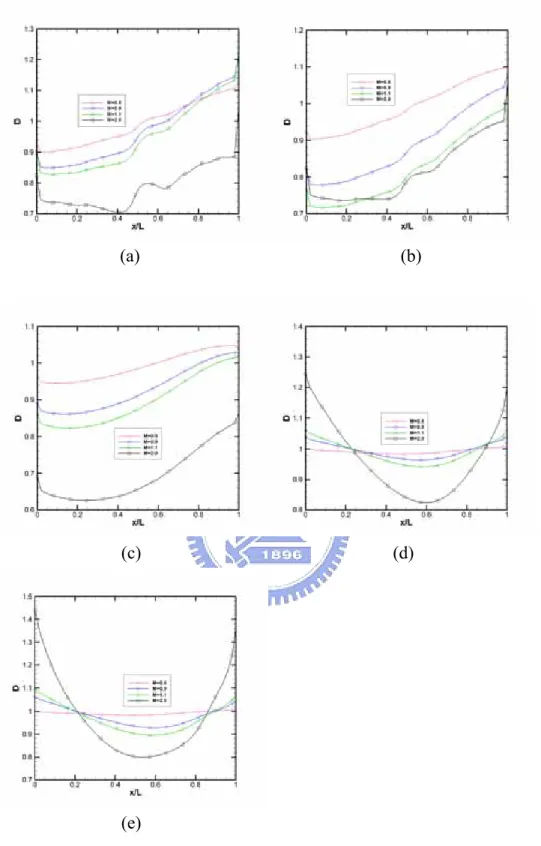
Results show that the velocity slips and temperature jumps increase at the solid walls with increasing rarefaction at the same Mach number. The vortex center move toward left and down as Knudsen number (Kn=10, 1, 0.1, 0.01) decreasing for M=0.5, 0.9, 1.1, and 2, when Kn=0.0033 is opposite. But the vortex center move toward the opposite way for M=0.5, Kn=0.0033 and M=2, Kn=0.0033. For Kn=0.01, and 0.0033, under the main vortex secondary eddies have been created at the two bottom corners. Only in this special example for M=2, Kn=10, unnder the main vortex secondary eddie have been created at the right bottom corners.

Table of Contents

Abstract ...IV Table of Contents ...VI List of Tables ... VIII List of Figures ...IX Nomenclature ... XVI

Chapter 1. Introduction ... 1

1.1 Motivation and Background ... 1

1.2 Literature Reviews in Driven Cavity Flows ... 4

1.3 Specific Objectives of the Thesis ... 6

Chapter 2. Numerical Method ... 7

2.1 Boltzmann equation ... 7

2.2 Model Boltzmann equation ... 9

2.2.1 BGK model ... 10

2.2.2 Ellipsoidal model ... 12

2.2.3 Shakov model ... 13

2.3 Discrete Ordinate Method ... 15

2.4 Finite-difference Discretization of the Two-Dimensional MBE ... 15

2.5 Numerical Algorithm in solving the MBE ... 24

Chapter 3. Preliminary Results and Discussion ... 32

3.1 Comparison of MBE Results with DSMC Numerical Method ... 32

The computed results using MBE are found to compare well with those using the DSMC(direct simulation Monte Carlo) in the Near-continuum regime flows . ... 32

3.2 Driven Cavity Flows ... 33

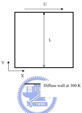
3.2.1 Problem Description and Test Conditions ... 33

3.2.2 Grid Convergence Tests ... 33

3.2.3 Effects of Knudsen Number ... 34

3.2.3.1 General Simulation Results ... 34

3.2.3.1.1 Subsonic Moving Plate (M=0.5, 0.9) ... 34

3.2.3.1.2 Supersonic Moving Plate (M=1.1, 2) ... 36

3.2.3.2 Property Distributions Across Cavity Centroid ... 38

3.2.3.3 Property Distributions Near Solid Walls ... 38

3.2.3.4 Recirculation Center Position ... 39

3.2.4 Effect of Mach Number of the Driven Plate ... 41

3.2.4.1.1 Free Molecular Regime (Kn=10) ... 41

3.2.4.1.2 Transitional Regime (Kn=1, 0.1, 0.01) ... 42

3.2.4.1.3 Near-continuum Regime (Kn=0.0033) ... 44

3.2.4.2 Property Distributions Across Cavity Centroid ... 46

3.2.4.3 Property Distributions Near Solid Walls ... 46

3.2.4.4 Recirculation Center Position ... 47

Chapter 4. Conclusions and Recommendation of Future Work ... 49

4.1 Conclusion ... 49

4.2 Recommendation of Future Work ... 50

List of Tables

Table. I All the Simulation cases. ... 53 Table. II Mesh information ... 54 Table. III Simulation condition ... 55 Table. IV Location of the center of the top vortex for various values of

List of Figures

Fig. 1.1 Flow Regime and solution method ... 57 Fig. 2.1 The Knudsen number limits on the mathematical models. ... 57 Fig. 3.1 The 2D square (L/H=1) driven cavity flow with moving top plate

58

Fig. 3.2 Grid. 1 is grid mesh of 101 by 101 and smallest grid size is

-3

10

5× . ... 59 Fig. 3.3 Grid. 2 is grid mesh of 101 by 101 and smallest grid size is

-3

10

1× _{... 60} Fig. 3.4 Grid. 3 is grid mesh of 201 by 201 and smallest grid size is

-3

10

5× _{... 61} Fig. 3.5 Grid. 4 is grid mesh of 101 by 101 and smallest grid size is

-2

10

1× _{... 62} Fig. 3.6 The residual functions for different grids (a) Grid. 1, (b) Grid. 2,

(c) Grid. 3, (d)Grid. 4. ... 63 Fig. 3.7 Contours of number Density for M=0.5, (a) Kn=10; (b) Kn=1; (c) Kn=0.1; (d) Kn=0.01; (e) Kn=0.0033 ... 64 Fig. 3.8 Contours of Temperature for M=0.5, (a) Kn=10; (b) Kn=1; (c)

Kn=0.1; (d) Kn=0.01; (e) Kn=0.0033 ... 65 Fig. 3.9 Contours of Mach number for M=0.5, (a) Kn=10; (b) Kn=1; (c)

Kn=0.1; (d) Kn=0.01; (e) Kn=0.0033 ... 66 Fig. 3.10 Contours of U-velocity for M=0.5, (a) Kn=10; (b) Kn=1; (c)

Kn=0.1; (d) Kn=0.01; (e) Kn=0.0033 ... 67 Fig. 3.11 Contours of V-velocity for M=0.5, (a) Kn=10; (b) Kn=1; (c)

Kn=0.1; (d) Kn=0.01; (e) Kn=0.0033 ... 68 Fig. 3.12 Contours of number Density for M=0.9, (a) Kn=10; (b) Kn=1; (c) Kn=0.1; (d) Kn=0.01; (e) Kn=0.0033 ... 69 Fig. 3.13 Contours of Temperature for M=0.9, (a) Kn=10; (b) Kn=1; (c)

Kn=0.1; (d) Kn=0.01; (e) Kn=0.0033 ... 70 Fig. 3.14 Contours of Mach number for M=0.9, (a) Kn=10; (b) Kn=1; (c)

Kn=0.1; (d) Kn=0.01; (e) Kn=0.0033 ... 71 Fig. 3.15 Contours of U-velocity for M=0.9, (a) Kn=10; (b) Kn=1; (c)

Kn=0.1; (d) Kn=0.01; (e) Kn=0.0033 ... 72 Fig. 3.16 Contours of V-velocity for M=0.9, (a) Kn=10; (b) Kn=1; (c)

Kn=0.1; (d) Kn=0.01; (e) Kn=0.0033 ... 73 Fig. 3.17 Contours of number Density for M=1.1, (a) Kn=10; (b) Kn=1; (c) Kn=0.1; (d) Kn=0.01; (e) Kn=0.0033 ... 74 Fig. 3.18 Contours of Temperature for M=1.1, (a) Kn=10; (b) Kn=1; (c)

Kn=0.1; (d) Kn=0.01; (e) Kn=0.0033 ... 75 Fig. 3.19 Contours of Mach number for M=1.1, (a) Kn=10; (b) Kn=1; (c)

Kn=0.1; (d) Kn=0.01; (e) Kn=0.0033 ... 76 Fig. 3.20 Contours of U-velocity for M=1.1, (a) Kn=10; (b) Kn=1; (c)

Kn=0.1; (d) Kn=0.01; (e) Kn=0.0033 ... 77 Fig. 3.21 Contours of V-velocity for M=1.1, (a) Kn=10; (b) Kn=1; (c)

Kn=0.1; (d) Kn=0.01; (e) Kn=0.0033 ... 78 Fig. 3.22 Contours of number Density for M=2.0, (a) Kn=10; (b) Kn=1; (c) Kn=0.1; (d) Kn=0.01; (e) Kn=0.0033 ... 79 Fig. 3.23 Contours of Temperature for M=2.0, (a) Kn=10; (b) Kn=1; (c)

Kn=0.1; (d) Kn=0.01; (e) Kn=0.0033 ... 80 Fig. 3.24 Contours of Mach number for M=2.0, (a) Kn=10; (b) Kn=1; (c)

Kn=0.1; (d) Kn=0.01; (e) Kn=0.0033 ... 81 Fig. 3.25 Contours of U-velocity for M=2.0, (a) Kn=10; (b) Kn=1; (c)

Kn=0.1; (d) Kn=0.01; (e) Kn=0.0033 ... 82 Fig. 3.26 Contours of V-velocity for M=2.0, (a) Kn=10; (b) Kn=1; (c)

Kn=0.1; (d) Kn=0.01; (e) Kn=0.0033 ... 83 Fig. 3.27 Profile of the number Density on a vertical plane x=0.5 for (a)

M=0.5; (b) M=0.9; (c) M=1.1; (d) M=2 ... 84 Fig. 3.28 Profile of the Temperature on a vertical plane x=0.5 for (a)

M=0.5; (b) M=0.9; (c) M=1.1; (d) M=2 ... 85 Fig. 3.29 Profile of the U-velocity on a vertical plane x=0.5 for (a) M=0.5; (b) M=0.9; (c) M=1.1; (d) M=2 ... 86 Fig. 3.30 Profile of the V-velocity on a vertical plane x=0.5 for (a) M=0.5; (b) M=0.9; (c) M=1.1; (d) M=2 ... 87 Fig. 3.31 Profile of the number Density on a horizontal plane y=-0.5 for (a) M=0.5; (b) M=0.9; (c) M=1.1; (d) M=2 ... 88 Fig. 3.32 Profile of the Temperature on a horizontal plane y=-0.5 for (a)

M=0.5; (b) M=0.9; (c) M=1.1; (d) M=2 ... 89 Fig. 3.33 Profile of the U-velocity on a horizontal plane y=-0.5 for (a)

M=0.5; (b) M=0.9; (c) M=1.1; (d) M=2 ... 90 Fig. 3.34 Profile of the V-velocity on a horizontal plane y=-0.5 for (a)

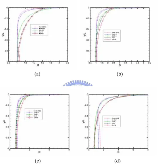
M=0.5; (b) M=0.9; (c) M=1.1; (d) M=2 ... 91 Fig. 3.35 Profile of the number Density on a vertical plane x=0 for (a)

M=0.5; (b) M=0.9; (c) M=1.1; (d) M=2 ... 92 Fig. 3.36 Profile of the Temperature on a vertical plane x=0 for (a) M=0.5; (b) M=0.9; (c) M=1.1; (d) M=2 ... 93 Fig. 3.37 Profile of the U-velocity on a vertical plane x=0 for (a) M=0.5;

(b) M=0.9; (c) M=1.1; (d) M=2 ... 94 Fig. 3.38 Profile of the V-velocity on a vertical plane x=0 for (a) M=0.5;

(b) M=0.9; (c) M=1.1; (d) M=2 ... 95 Fig. 3.39 Profile of the number Density on a vertical plane x=1 for (a)

M=0.5; (b) M=0.9; (c) M=1.1; (d) M=2 ... 96 Fig. 3.40 Profile of the Temperature on a vertical plane x=1 for (a) M=0.5; (b) M=0.9; (c) M=1.1; (d) M=2 ... 97 Fig. 3.41 Profile of the U-velocity on a vertical plane x=1 for (a) M=0.5;

(b) M=0.9; (c) M=1.1; (d) M=2 ... 98 Fig. 3.42 Profile of the V-velocity on a vertical plane x=1 for (a) M=0.5;

(b) M=0.9; (c) M=1.1; (d) M=2 ... 99 Fig. 3.43 Profile of the number Density on a horizontal plane y=-1 for (a)

M=0.5; (b) M=0.9; (c) M=1.1; (d) M=2 ... 100 Fig. 3.44 Profile of the Temperature on a horizontal plane y=-1 for (a)

M=0.5; (b) M=0.9; (c) M=1.1; (d) M=2 ... 101 Fig. 3.45 Profile of the U-velocity on a horizontal plane y=-1 for (a)

M=0.5; (b) M=0.9; (c) M=1.1; (d) M=2 ... 102 Fig. 3.46 Profile of the V-velocity on a horizontal plane y=-1 for (a)

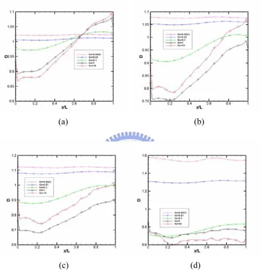
M=0.5; (b) M=0.9; (c) M=1.1; (d) M=2 ... 103 Fig. 3.47 Profile of the number Density on a horizontal plane y=0 for (a)

M=0.5; (b) M=0.9; (c) M=1.1; (d) M=2 ... 104 Fig. 3.48 Profile of the Temperature on a horizontal plane y=0 for (a)

M=0.5; (b) M=0.9; (c) M=1.1; (d) M=2 ... 105 Fig. 3.49 Profile of the U-velocity on a horizontal plane y=0 for (a)

M=0.5; (b) M=0.9; (c) M=1.1; (d) M=2 ... 106 Fig. 3.50 Profile of the V-velocity on a horizontal plane y=0 for (a)

M=0.5; (b) M=0.9; (c) M=1.1; (d) M=2 ... 107 Fig. 3.51 Velocity streamlines for M=0.5, and (a) Kn=10; (b) Kn=1; (c)

Kn=0.1; (d) Kn=0.01; (e) Kn=0.0033 ... 108 Fig. 3.52 Velocity streamlines for M=0.9, and (a) Kn=10; (b) Kn=1; (c)

Kn=0.1; (d) Kn=0.01; (e) Kn=0.0033 ... 109 Fig. 3.53 Velocity streamlines for M=1.1, and (a) Kn=10; (b) Kn=1; (c)

Kn=0.1; (d) Kn=0.01; (e) Kn=0.0033 ... 110 Fig. 3.54 Velocity streamlines for M=2, and (a) Kn=10; (b) Kn=1; (c)

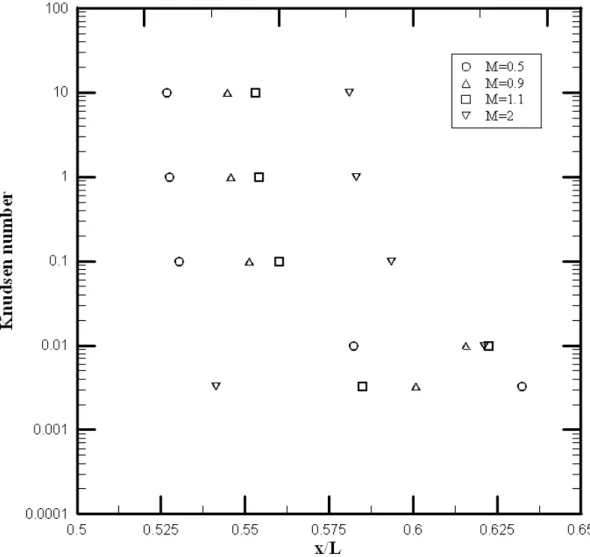
Kn=0.1; (d) Kn=0.01; (e) Kn=0.0033 ... 111 Fig. 3.55 Location of the center for x/L of the top vortex for various

values of Mach number and Knudsen number. ... 112 Fig. 3.56 Location of the center for y/L of the top vortex for various

values of Mach number and Knudsen number. ... 113 Fig. 3.57 Contours of number Density for Kn=10, (a) M=0.5; (b) M=0.9;

(c) M=1.1; (d) M=2.0 ... 114 Fig. 3.58 Contours of Temperature for Kn=10, (a) M=0.5; (b) M=0.9; (c)

M=1.1; (d) M=2.0 ... 115 Fig. 3.59 Contours of Mach number for Kn=10, (a) M=0.5; (b) M=0.9; (c) M=1.1; (d) M=2.0 ... 116 Fig. 3.60 Contours of U-velocity for Kn=10, (a) M=0.5; (b) M=0.9; (c)

M=1.1; (d) M=2.0 ... 117 Fig. 3.61 Contours of V-velocity for Kn=10, (a) M=0.5; (b) M=0.9; (c)

M=1.1; (d) M=2.0 ... 118 Fig. 3.62 Contours of number Density for Kn=1, (a) M=0.5; (b) M=0.9; (c) M=1.1; (d) M=2.0 ... 119 Fig. 3.63 Contours of Temperature for Kn=1, (a) M=0.5; (b) M=0.9; (c)

M=1.1; (d) M=2.0 ... 120 Fig. 3.64 Contours of Mach number for Kn=1, (a) M=0.5; (b) M=0.9; (c)

M=1.1; (d) M=2.0 ... 121 Fig. 3.65 Contours of U-velocity for Kn=1, (a) M=0.5; (b) M=0.9; (c)

M=1.1; (d) M=2.0 ... 122 Fig. 3.66 Contours of V-velocity for Kn=1, (a) M=0.5; (b) M=0.9; (c)

M=1.1; (d) M=2.0 ... 123 Fig. 3.67 Contours of number Density for Kn=0.1, (a) M=0.5; (b) M=0.9;

(c) M=1.1; (d) M=2.0 ... 124 Fig. 3.68 Contours of Temperature for Kn=0.1, (a) M=0.5; (b) M=0.9; (c)

M=1.1; (d) M=2.0 ... 125 Fig. 3.69 Contours of Mach number for Kn=0.1, (a) M=0.5; (b) M=0.9; (c) M=1.1; (d) M=2.0 ... 126 Fig. 3.70 Contours of U-velocity for Kn=0.1, (a) M=0.5; (b) M=0.9; (c)

M=1.1; (d) M=2.0 ... 127 Fig. 3.71 Contours of V-velocity for Kn=0.1, (a) M=0.5; (b) M=0.9; (c)

M=1.1; (d) M=2.0 ... 128 Fig. 3.72 Contours of number Density for Kn=0.01, (a) M=0.5; (b) M=0.9; (c) M=1.1; (d) M=2.0 ... 129 Fig. 3.73 Contours of Temperature for Kn=0.01, (a) M=0.5; (b) M=0.9; (c)

M=1.1; (d) M=2.0 ... 130 Fig. 3.74 Contours of Mach number for Kn=0.01, (a) M=0.5; (b) M=0.9;

(c) M=1.1; (d) M=2.0 ... 131 Fig. 3.75 Contours of U-velocity for Kn=0.01, (a) M=0.5; (b) M=0.9; (c)

M=1.1; (d) M=2.0 ... 132 Fig. 3.76 Contours of V-velocity for Kn=0.01, (a) M=0.5; (b) M=0.9; (c)

M=1.1; (d) M=2.0 ... 133 Fig. 3.77 Contours of number Density for Kn=0.0033, (a) M=0.5; (b)

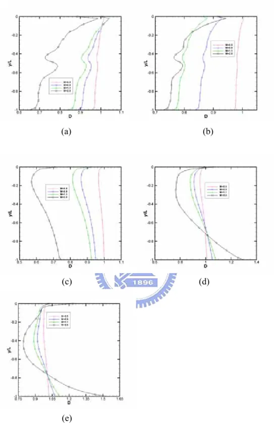
M=0.9; (c) M=1.1; (d) M=2.0 ... 134 Fig. 3.78 Contours of Temperature for Kn=0.0033, (a) M=0.5; (b) M=0.9; (c) M=1.1; (d) M=2.0 ... 135 Fig. 3.79 Contours of Mach number for Kn=0.0033, (a) M=0.5; (b) M=0.9; (c) M=1.1; (d) M=2.0 ... 136 Fig. 3.80 Contours of U-velocity for Kn=0.0033, (a) M=0.5; (b) M=0.9; (c) M=1.1; (d) M=2.0 ... 137 Fig. 3.81 Contours of V-velocity for Kn=0.0033, (a) M=0.5; (b) M=0.9; (c) M=1.1; (d) M=2.0 ... 138 Fig. 3.82 Profile of the number Density on a vertical plane x=0.5 for (a)

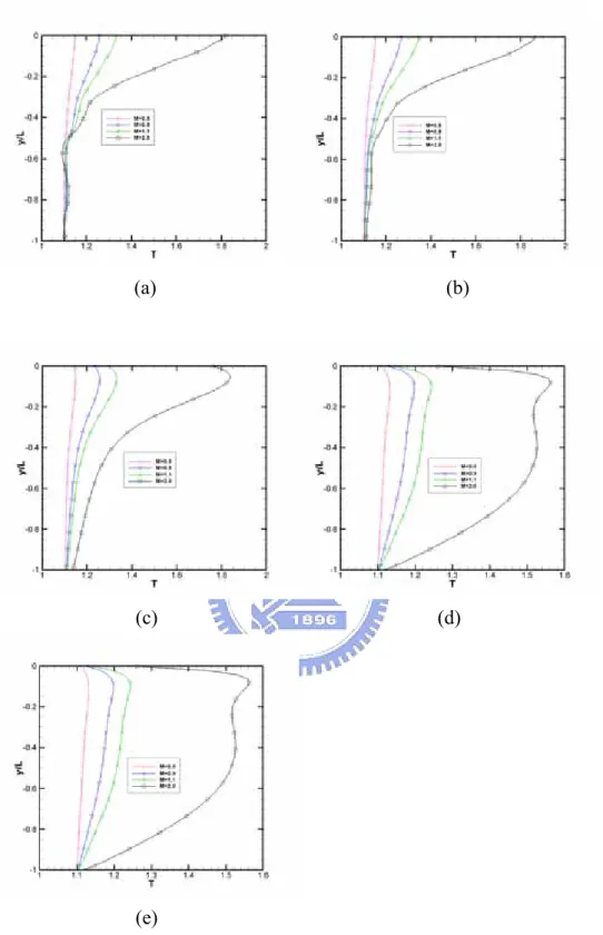
Kn=10; (b) Kn=1; (c) Kn=0.1; (d) Kn=0.01; (e) Kn=0.0033 ... 139 Fig. 3.83 Profile of the Temperature on a vertical plane x=0.5 for (a)

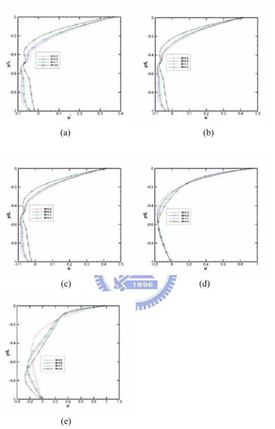
Kn=10; (b) Kn=1; (c) Kn=0.1; (d) Kn=0.01; (e) Kn=0.0033 ... 140 Fig. 3.84 Profile of the U-velocity on a vertical plane x=0.5 for (a) Kn=10; (b) Kn=1; (c) Kn=0.1; (d) Kn=0.01; (e) Kn=0.0033 ... 141 Fig. 3.85 Profile of the V-velocity on a vertical plane x=0.5 for (a) Kn=10; (b) Kn=1; (c) Kn=0.1; (d) Kn=0.01; (e) Kn=0.0033 ... 142 Fig. 3.86 Profile of the number Density on a horizontal plane y=-0.5 for (a) Kn=10; (b) Kn=1; (c) Kn=0.1; (d) Kn=0.01; (e) Kn=0.0033 ... 143 Fig. 3.87 Profile of the Temperature on a horizontal plane y=-0.5 for (a)

Kn=10; (b) Kn=1; (c) Kn=0.1; (d) Kn=0.01; (e) Kn=0.0033 ... 144 Fig. 3.88 Profile of the U-velocity on a horizontal plane y=-0.5 for (a)

Kn=10; (b) Kn=1; (c) Kn=0.1; (d) Kn=0.01; (e) Kn=0.0033 ... 145 Fig. 3.89 Profile of the V-velocity on a horizontal plane y=-0.5 for (a)

Kn=10; (b) Kn=1; (c) Kn=0.1; (d) Kn=0.01; (e) Kn=0.0033 ... 146 Fig. 3.90 Profile of the number Density on a vertical plane x=0 for (a)

Kn=10; (b) Kn=1; (c) Kn=0.1; (d) Kn=0.01; (e) Kn=0.0033 ... 147 Fig. 3.91 Profile of the Temperature on a vertical plane x=0 for (a) Kn=10; (b) Kn=1; (c) Kn=0.1; (d) Kn=0.01; (e) Kn=0.0033 ... 148 Fig. 3.92 Profile of the U-velocity on a vertical plane x=0 for (a) Kn=10;

(b) Kn=1; (c) Kn=0.1; (d) Kn=0.01; (e) Kn=0.0033 ... 149 Fig. 3.93 Profile of the V-velocity on a vertical plane x=0 for (a) Kn=10;

(b) Kn=1; (c) Kn=0.1; (d) Kn=0.01; (e) Kn=0.0033 ... 150 Fig. 3.94 Profile of the number Density on a vertical plane x=1 for (a)

Kn=10; (b) Kn=1; (c) Kn=0.1; (d) Kn=0.01; (e) Kn=0.0033 ... 151 Fig. 3.95 Profile of the Temperature on a vertical plane x=1 for (a) Kn=10; (b) Kn=1; (c) Kn=0.1; (d) Kn=0.01; (e) Kn=0.0033 ... 152 Fig. 3.96 Profile of the U-velocity on a vertical plane x=1 for (a) Kn=10;

(b) Kn=1; (c) Kn=0.1; (d) Kn=0.01; (e) Kn=0.0033 ... 153 Fig. 3.97 Profile of the V-velocity on a vertical plane x=1 for (a) Kn=10;

(b) Kn=1; (c) Kn=0.1; (d) Kn=0.01; (e) Kn=0.0033 ... 154 Fig. 3.98 Profile of the number Density on a horizontal plane y=-1 for (a)

Kn=10; (b) Kn=1; (c) Kn=0.1; (d) Kn=0.01; (e) Kn=0.0033 ... 155 Fig. 3.99 Profile of the Temperature on a horizontal plane y=-1 for (a)

Kn=10; (b) Kn=1; (c) Kn=0.1; (d) Kn=0.01; (e) Kn=0.0033 ... 156 Fig. 3.100 Profile of the U-velocity on a horizontal plane y=-1 for (a)

Kn=10; (b) Kn=1; (c) Kn=0.1; (d) Kn=0.01; (e) Kn=0.0033 ... 157 Fig. 3.101 Profile of the V-velocity on a horizontal plane y=-1 for (a)

Kn=10; (b) Kn=1; (c) Kn=0.1; (d) Kn=0.01; (e) Kn=0.0033 ... 158 Fig. 3.102 Profile of the number Density on a horizontal plane y=0 for (a)

Kn=10; (b) Kn=1; (c) Kn=0.1; (d) Kn=0.01; (e) Kn=0.0033 ... 159 Fig. 3.103 Profile of the Temperature on a horizontal plane y=0 for (a)

Kn=10; (b) Kn=1; (c) Kn=0.1; (d) Kn=0.01; (e) Kn=0.0033 ... 160 Fig. 3.104 Profile of the U-velocity on a horizontal plane y=0 for (a)

Kn=10; (b) Kn=1; (c) Kn=0.1; (d) Kn=0.01; (e) Kn=0.0033 ... 161 Fig. 3.105 Profile of the V-velocity on a horizontal plane y=0 for (a)

Kn=10; (b) Kn=1; (c) Kn=0.1; (d) Kn=0.01; (e) Kn=0.0033 ... 162 Fig. 3.106 Velocity streamlines for Kn=10, and (a) M=0.5; (b) M=0.9; (c)

M=1.1; (d) M=2.0 ... 163 Fig. 3.107 Velocity streamlines for Kn=1, and (a) M=0.5; (b) M=0.9; (c)

M=1.1; (d) M=2.0 ... 164 Fig. 3.108 Velocity streamlines for Kn=0.1, and (a) M=0.5; (b) M=0.9; (c) M=1.1; (d) M=2.0 ... 165 Fig. 3.109 Velocity streamlines for Kn=0.01, and (a) M=0.5; (b) M=0.9;

(c) M=1.1; (d) M=2.0 ... 166 Fig. 3.110 Velocity streamlines for Kn=0.0033, and (a) M=0.5; (b) M=0.9; (c) M=1.1; (d) M=2.0 ... 167 Fig. 3.111 Location of the center for x/L of the top vortex for various

values of Mach number and Knudsen number. ... 168 Fig. 3.112 Location of the center for y/L of the top vortex for various

values of Mach number and Knudsen number. ... 169 Fig. 3.113 Properties of M=0.9, Kn=0.0033 using UNIC for (a) number

density, (b) temperature, (c) Mach number, (d) u-velocity, (e)

v-velocity, (f) velocity streamlines. ... 170 Fig. 3.114 Properties of M=2, Kn=0.0033 using DSMC for (a) number

density, (b) temperature, (c) Mach number, (d) u-velocity, (e)

Nomenclature

λ ：mean free path ρ ：density

δ ：Kronecker delta

δ ：the Dirac delta function

σ ：the differential cross section

μ ：coefficient of viscosity

χ ：deflection angle

ν ：collision rate

ξ ：transformed xˆ coordinate

η ：transformed yˆ coordinate

τ ：viscous stress, relaxation time Ω : space domain

Ut ：time-step

σT ：the total cross section

c ：random velocity e ：specific energy

f ：normalized velocity distribution function in velocity soace

M

f ：Maxwellian velocity distribution

g,h,j,k ：reduced distribution function k ：the Boltzmann constant

Kn : Knudsen number L ：characteristic length; m ：molecule mass M ：mach number n ：number density r P : Prandtl number R ：gas constant Re ：Reynolds number u ：mean velocity

Chapter 1. Introduction

1.1 Motivation and Background

The driven cavity flow is one of the benchmark problems often used in computational fluid dynamics due to its simple geometry but highly singular points at the corners. It is often used to verify different numerical methods for fluid-flow simulation. However, past studies in this regard focused on flows in thc continuum regime. Very few researches have been done systematically in the rarefied or near-contiuum regime. Several applications require consideration of rarefaction on the flow fields, which motivates the present thesis to focus on the simulations of driven cavity flows in this region.

It is well known that continuum Navier-Stokes equations fails in treating these non-equilibrium effects in the transitional regime and beyond, as shown in Fig. 1.1. Even Navier-Stokes equation was often used with slip boundary conditions at walls for slightly rarefied flows, it is still uncertain how accurate they are and how far into the rarfied regime they can be applied. Thus, the Boltzmann equation based on the kinetic theory of gases needs to be used in these regimes. Due to the complexity of the nonlinear integral-differential nature of the equation, analytical solutions of the Boltzmann equation are rarely seen, hence numerical solutions is necessary.

exist two classes of methods. The first one is a probabilistic approach, such as the direct simulation Monte Carlo method (DSMC) [Bird’s book, 1994], which has been proved mathematically that it solves Boltzmann equation as the number simulated particles becomes large [Wagner, 1992; Nanbu, 1986]. It is the most commonly used numerical method for solving the Boltzmann equation. DSMC was found to be very efficient and accurate in high-speed gas flows.. However, high statistical uncertainties arise for low-speed gas flows, near-continuum flows, and unsteady flow, to name a few. To obtain acceptable solution with low noise, tremendous computing power is required for the DSMC simulation, which is unpractical. The second approach is a deterministic approach, such as numerically solving Boltzmann equation. This class includes the model Boltzmann equation, which is the main theme of the present thesis or the direct Boltzmann equation solver, which is still in its infant stage and beyond the scope of the present thesis.

The difficulties encountered in the solution of the Boltzmann equation are largely associated with the nonlinear integral nature of the collision term. To circumvent this difficulty, statistical or relaxation models were often proposed as substitutions. The kinetic model equation proposed by Krook et al. (BGK) [1954] and Welander [1954] provides a more tractable way to solve comparatively complex rarefied gas problems routinely. Several model equations for the nonlinear Boltzmann equation

have been proposed such as the ellipsoidal model by Holway [1963], by Cercignani and Tironi [1967] and high order generalization of the BGK model by Shakhov [1968]. A hierarchy kinetic model equation similar to that of Shakhov was also proposed by Abe and Oguchi [1976]. Among the main features of these high order generalizations of BGK model are that they give the correct Prandtl number and it is generally believed that they should give a solution much closer to the solution with the Boltzmann equation than the BGK model does. All these model equations bear a resemblance to the original Boltzmann equation concerning the various order of moments. Thus, instead of solving the full Boltzmann equation one solves the kinetic model equation and hopes to produce a more economic and efficient way of computing rarefied gasdynamic flows. Recent numerical studies of rarefied gas flow problems based on the BGK type model Boltzmann equations can be found in Sugimoto and Sone [1992] and Prendergast and Xu [1993]. We consider an accurate numerical method for solving the kinetic model Boltzmann equation. The approach taken here is to apply the discrete ordinate method Huang and Giddens [1967]; Shizgal [1981] to the distribution function to replace its continuous dependency on the velocity space by a set of distribution functions which are continuous function in physical space and time but point function in velocity space. The resulting set of partial differential equations are of hyperbolic type and can be cast into hyperbolic

conservation laws from with nonlinear source terms. Once this is done, modern upwind high resolution shock capturing methods can be applied to solve them. Here, we extend our previous high-order nonoscillatory method [Yang, 1991; Yang and Hsu, 1992] for hyperbolic conservation laws to include the nonlinear source term. [Yang and Huang, 1995] was to present a high resolution numerical method for the computation of rarefied gas flow over obstacles of arbitrary shapes covering the full spectrum of flow regimes using kinetic model Boltzmann equation. They method provided an efficient tool for accurate simulations of steady and unsteady rarefied gas flows covering the full spectrum of flow regimes and can contribute to the database by providing the results of simulations based upon the kinetic model Boltzmann equations.

1.2 Literature Reviews in Driven Cavity Flows

Ghia [1982] used Navier-Stokes equations to simulate the driven cavity flow with high Reynolds number. Solutions are obtained for configurations with Reynolds number as high as 10000 and meshes consisting of as many as 257×257 point. Detailed accurate results have been presented for this problem and the results agree well with published fine-grid solutions but are about four times as efficient.

Erturk et al. [2005] used Navier-Stokes equations to simulate the 2-D steady incompressible driven cavity flow. Solution are obtained for configurations with

Reynolds number ≤ 21,000 and using a fine uniform grid mesh of 601×601 cells. A new quaternary vortex at the bottom left corner and a new tertiary vortex at the top corner of the cavity are observed in the flow field as the Reynolds number increases. Naris and Valougeorgis [2005] used the two–dimensional linearized Bhatnagar-Gross-Krook (BGK) kinetic equation with Maxwell diffuse-specular boundary conditions to simulate the flow of a rarefied gas in a rectangular enclosure due to the motion of the upper wall is solved over the whole range of the Knudsen number. The integro-differential equations are solved numerically implementing the discrete velocity method. The discontinuity at the boundaries between stationary and moving walls is treated accordingly. A detailed investigation of the rarefaction effects on the flow pattern and quantities is presented over the whole range of the Knudsen number and various aspect (height/width) ratios. As the depth of the cavity is increased, these eddies grow and merge into additional vortices under the top one. As Knudsen number decreased, the center of the top vortex is move slightly toward the moving wall.

1.3 Specific Objectives of the Thesis

Based on previous reviews, the current objectives of the thesis are summarized as

follows:

1. To benchmark the solution obtained by the previously developed 2D MBE solver with that obtained by the DMSC method;

2. To utilize the above validated 2D MBE solver to study the driven cavity flows in detail with Mach number and Knudsen number in the range of 0.5-2 and 10-0.0033, respectively.

3. To discuss the results considering the effects of rarefaction and compressibility.

The organization of the thesis would be stated as follows. First is this introduction, and next is the numerical method. Then simulation results of Model Boltzmann equation are presented. Finally, conclusion and recommendation of future work are presented.

Chapter 2. Numerical Method

The degree of rarefaction of a gas is generally expressed through the Knudsen number (Kn) which is the ratio of the mean free path λ to the characteristic dimension L ; i.e.

( )

Kn =λ_L (2.1) Traditionally, flows are divided into four regimes as follows: Kn<0.01 (continuum), 0.01<Kn<0.1 (slip flow), 0.1<Kn<3 (transitional flow) and Kn>3 (free molecular flow). As the Kn increases, the rarefaction becomes important and even dominates the flow behavior. Hence, the traditional requirement for the Navier-Stokes equations to be valid is that Knudsen number should be less than 0.1. (Figure 2.1)

2.1 Boltzmann equation

The Boltzmann equation is one of the most important transport equations in non-equilibrium statistical mechanics, which deals with systems far from thermodynamics equilibrium. There are some assumptions made in the derivation of the Boltzmann equation which defines limits of applicability. They are summarized as follows:

1. Molecular chaos is assumed which is valid when the intermolecular forces are short range. It allows the representation of the two particles distribution function as a product of the two single particle distribution functions.

2. Distribution functions do not change before particle collision. This implies that the encounter is of short time duration in comparison to the mean free collision time.

3. All collisions are binary collisions.

4. Particles are uninfluenced by intermolecular potentials external to an interaction.

According to these assumptions, the Boltzmann equation is derived and shown as Eq. (2.1) 4 2 ' ' 1 1 0 ( ) ( ) ( ) ( ) i i c i i i nf nf nf f u F n f f ff g d dU t x u x π σ ∞ −∞ ∂ ₊ ∂ ₊ ∂ ₌ ∂ _{= − Ω} ∂ ∂ ∂ ∂

∫ ∫

(2.1)

Meaning of particle phase-space distribution function f is the number of particles with center of mass located within a small volume 3

d r near the point r , and

velocity within a range 3

d u , at time t . F is an external force per unit mass and t _i

is the time and u is the molecular velocity. _i σ is the differential cross section and

dΩ is an element of solid angle. The prime denotes the post-collision quantities

and the subscript 1 denotes the collision partner. Meaning of each term in Eq. (2.1) is described in the following;

1. The first term on the left hand side of the equation represents the time variation of the distribution function of the particles (unsteady term).

term).

3. The third term describes the effect of a force on the particles (force term). 4. The term at right hand side of the equation is called the collision integral

(collision term). It is the source of most of the difficulties in obtaining solutions of the Boltzmann equation.

In general, it is very hard to solve the Boltzmann equation directly using numerical method because the difficulties of correctly modeling the integral collision term. Instead, the DSMC method was used to simulated problems involving rarefied gas dynamics, which is the simulation tool used in the current thesis.

2.2 Model Boltzmann equation

Because of the complex nonlinear structure of the collision integral, the Boltzmann equation is very difficult to solve and to analyze, which is a nonlinear integral-differential equation. Since the Boltzmann equation is difficult to handle, and its numerical solution is time expensive, some alternative, simpler expressions have been proposed to replace the Boltzmann collision term. These are known as collision models, and any Boltzmann-like equation where the Boltzmann collision integral is replaced by a collision model is called a model equation or a kinetic model.

2.2.1 BGK model

The most widely known collision model is usually called the Bhatnagar, Gross and Krook (BGK) model. We approximate the collision term in the Boltzmann equation become: f) -(f ] t f [ M coll. =ν ∂ ∂ (2.2) Where _{f is the Maxwellian distribution function,}M _{and ν is the proportion}

coefficient of the BGK equation, which is also named as the collision frequency. The power law temperature dependence of the coefficient of viscosity can be obtained [,] from the Chapman–Enskog theory, which is appropriate for the inverse power law intermolecular force model and the VHS (Variable Hard Sphere) molecular model,

χ µ µ ) T T ( ref ref = (2.3) Where χ is the temperature exponent of the coefficient of viscosity that can also be denoted as

₍

₎

1 -2 3 ζ ζ

χ= + for the Chapman–Enskog gas of inverse power law, f is the inverse power coefficient related to the power force and the distance between centers of molecules, RT 2 mn 5 16 π µ λ= (2.4) Where m is the molecular mass, R is the gas constant, λ is the mean free path. The nominal collision frequency (inverse relaxation time) can be taken in the form

µ

ν =nkT (2.5) Where n is the number density, k is Boltzmann’s constant (k =R⋅m), and µ is the coefficient of the viscosity.

The BGK collision model equation [] was proposed by replacing the collision integral term of the Boltzmann equation with simple collision model:

(

f -f

)

v f a r f v t f ₌

_ν

M ∂ ∂ ⋅ + ∂ ∂ ⋅ + ∂ ∂ v v v v _(2.6)

wheref( vvr ,v, t)is the velocity distribution function which depends on space, rv , molecular velocity, vv , and time, t; ν is the collision frequency and _{f is the local} M

Maxwellian equilibrium distribution function given by ] t) , r 2RT( t)) , r u( -v ( t)) , r RT( (2 t) , r n( t) , v , r ( f 2 2 3 M v v v v v v v π = (2.7)

The idea behind this replacement is that a large amount of detail of the two-body interaction (which is contained in the collision term) is not likely to influence significantly the values of many experimentally measured quantities. That is, unless very refined experiments are devised, it is expected that the fine structure of the collision operator can be replace by a blurred image, based upon a simpler operator which retains only the qualitative and average properties of the true collision operator. The numerical method uses the BGK equation as the starting point for the computation, the molecular velocity distribution function is chosen as the dependent variable, the single velocity distribution function equation can be transformed into the

hyperbolic conservation equations to be numerically solved with the finite difference method in computational fluid dynamics by the aid of the discrete velocity ordinate method in gas kinetic theory, and then the macroscopic flow variables at each point in the physical space can be evaluated from the moments of the distribution function over the velocity space.

2.2.2 Ellipsoidal model

Although that, the most widely known collision model is usually called the BGK model. But the BGK model gives the value P_r =1 for the Prandtl number, a value which is not in agreement with both the true Boltzmann equation and the experimental data for a monatomic gas (which agree in giving P_r ≈ 2₃). Therefore, Holway (1966) and Cercignani (1967) had created a new model about model Boltzmann equation is called ellipsoidal statistical (ES) model equation.

P_r is the Prandtl number with

k c

P_r = p µ , C is the specific heat at constant _p pressure, µ is the coefficient of the viscosity, k is the heat conduction coefficient. In order to have a correct value for the Prandtl number, the Maxwellian distribution function _{f in the BGK equation can be replaced by Three-dimensional} M

Anisotropic Gaussian Distribution in the Ellipsoidal model.

(

f

-

f

)

v

f

a

r

f

v

t

f

₌

_ν

E

∂

∂

⋅

+

∂

∂

⋅

+

∂

∂

v

v

v

v

(2.8)

(

)

(

)

_⎥ ⎦ ⎤ ⎢ ⎣ ⎡ =

∑

= 3 1 j i, j i ij 2 1 2 3 -E _{v,r,t det A exp - A cc} f v v

ρπ

_(2.9a)

(

)

( )

-1 r ij r ij r ij P P P -1 2 -P 2RT A A ρ δ ⎟⎟ ⎠ ⎞ ⎜⎜ ⎝ ⎛ = = (2.9b)

Where δ_ij is the Kronecker delta such that

j i , 1 j i , 0 ij

{

= ≠

=

δ

_(2.9c)

Ellipsoidal model had be proof better than BGK model in solve some shock structure problems. However, A disadvantage of this model is that it has not been possible to prove (or disprove) the H theory.

2.2.3 Shakov model

In order to have a correct value for the Prandtl number, higher-order equation, namely, the Shakhov equation, as well as the complete Boltzmann equation, is usually used in the numerical solution. Neglect external force after the function, the Boltzmann equation become;

(

f -f

)

] t f [ r f v t f coll. + = ∂ ∂ = ∂ ∂ ⋅ + ∂ ∂

_ν

v v _(2.10)

∫

= f₁v_rσdvv₁ ν (2.10a) ν + + ₌J f (2.10b) dv d v f f f * _{r 1} 1 * _Ω =

∫

+ _(2.10c)

proportion to relative velocity among the molecules v_r, namely collide frequency is not the function of the molecule velocity, the model Shakhov equation can be write this type;

(

f -f

)

r f v t f ₌

_ν

S ∂ ∂ ⋅ + ∂ ∂ v v _(2.11)

Where _{f is the local Maxwellian equilibrium distribution function given by} S

5)/(5pRT)] -RT c q( Pr)c -(1 t)[1 , v , r ( f t) , v , r ( f 2 M S v v ₌ v v _{+ ⋅ (2.12)}

If moment equation for Eq. (2.11) is same as moment equation for Eq. (2.10), which model equation (2.11) is similar equation for Boltzmann equation (2.10).

∫

∫

= ∂_∂ ] dv t f [ v d f) -(fs _ψ v _coll.ψ v ν (2.13) Where ψ =ψ(vv )=1, v_i, v_iv_j, v_iv_jv_k,... (2.14a) Alternatively one can use ψ =ψ(vv )=1,c_i ,c_ic_j ,c_ic_jc_k,... (2.14b) We assume that ...} c a c a c a {a f f (3) _ijk ijk ij (2) ij i (1) i (0) M S _{= + + + + (2.15)}

We consider Eq. (2.15) reduced

The Shakhov model kinetic equation is a generalization of the Krook model equation in that the approximation condition is satisfied not only for 2 _{i j}

i, v ,vv

v 1,

but also for 2 iv

v . This ensures the correct relaxation of both the heat flux and stresses, leading thus to the correct continuum limit in the case of small Knudsen numbers. In particular, the model gives the correct Prandtle number. Comparisons of different monatomic model equations with experimental data and the finite-difference solution

to be more accurate than the BGK model and Ellipsoidal models.

2.3 Discrete Ordinate Method

We consider accurate numerical methods for solving the kinetic model Boltzmann equations. The approach taken here is to apply the discrete ordinate method to the distribution function to replace its continuous dependency on the velocity space by a set of distribution functions which are continuous function in physical space and time but point function in velocity space. The resulting set of partial differential equations are of hyperbolic type and can be cast into hyperbolic conservation laws from with nonlinear source terms.

Its main idea is to replace the exact integration with respect to molecular velocity v over all velocity space by an approximate numerical integration over a finite domain using a discrete set of points. Let β be an index of the three-

dimensional molecular velocity mesh, v be a node in this mesh,_β f_β =f(t,rv,v_β). Then the model kinetic equation is replaced by a system of equations for f . _β

2.4 Finite-difference Discretization of the Two-Dimensional MBE We consider a class of model Boltzmann equations of the form

(

f -f

)

r f v t f ₌

_ν

N ∂ ∂ ⋅ + ∂ ∂ v v _(2.16)

wheref( vrv ,v, t)is the velocity distribution function which depends on space, rv , molecular velocity, vv , and time, t; ν is the collision frequency and _{f is an} N

appropriate distribution function depending on the model selected. The number density, macroscopic flow velocity, and temperature of the gas are the first three moments of the distribution function

∫

= f(r ,v, t)d v t) , r n(v v v 3 _(2.17) 3 2, 1, i , v d t) , v , r f( v t) , r ( nu 3 i i v =

∫

v v = (2.18)

∫

= f(r ,v, t)d v 2 c 2 t) , r 3nRT(v 2 v v 3 _(2.19)

Here, R is the gas constant, c=vv -u(vr, t)is the peculiar velocity of the molecule. The gas pressure p and the stress tensor τ_ij are defined by

t) , r t)kT( , r n( t) , r p(v = v v (2.20)

∫

= ij 3 j i ij(r, t) c c f(r ,v, t) d v-pδ τ v v v (2.21)

where k is the Boltzmann constant and δ_ij is the Kronecker delta. The heat flux vector q is

∫

= cf(r ,v, t)d v 2 c t) , r ( q 3 i 2 i v v v (2.22)

The elastic collision frequency is of the form µ

ν =nkT (2.23)

where µ is the viscosity and is assumed to have a temperature dependence

χ

µ

Here χ is a constant for a given gas. If we assume the dependence of the viscosity on the temperature as for the Chapmann-Enskog gas of inverse ζ power law, we have

₍

₎

1 -2 3 ζ ζ

χ= + . For Maxwell molecules, ζ =5 then χ =1.; thus the collision frequency is independent of temperature. The viscosity coefficient µ is related to _∞ the freestream mean free path λ by the relation _∞

∞ ∞ ∞ ∞ = RT 2 mn 5 16 π λ µ (2.25)

In this study we consider two kinetic models for _{f ; one is the BGK model and the} N

other is the Shakov model. For the BGK model, we have _{f equal to the Maxwellian} N

distribution _{f :} M ] t) , r 2RT( t)) , r u( -v ( t)) , r RT( (2 t) , r n( t) , v , r ( f f 2 2 3 M N v v v v v v v π = = (2.26)

For the Shakov model, we have

5)/(5pRT)] -RT c q( Pr)c -(1 t)[1 , v , r ( f t) , v , r ( f f 2 M S N ₌ v v ₌ v v _{+ ⋅ (2.27)}

Here, Pr is the prandtl number and is equal to 3 2

for a monatomic gas.

We note that the derivation of the continuum Navier-Stokes equations from the BGK model or the Shakov model can be obtained using a Chapmann-Enskog procedure.

To illustrate the numerical approach, we describe in detail the relevant equations for two-dimensional problem, for the purpose of reduction in computer storage requirements, the following reduced distribution functions (Chu 1965) are introduced:

z -y x,v ,x,y,t) f(v,x,y,t)dv g(v

∫

∞ ∞ = v (2.28a) z -2 z y x,v ,x,y,t) v f(v,x,y,t)dv h(v

∫

∞ ∞ = v (2.28b)

Define the reference velocity and time as C_∞ = 2RT_∞ t_∞ =L C_∞

Where L is the reference length, T_∞ is the reference temperature. Then, the non-dimensional variables can be defined as follows:

L y yˆ , L x xˆ , ) C (mn ˆ , ) C mn 2 1 ( q qˆ , ) C mn 2 1 ( P Pˆ , T T Tˆ n n nˆ , C v vˆ , C u uˆ , C u uˆ , t t t ˆ 2 ij ij 3 x 2 i i y y x x = = = = = = = = = = = ∞ ∞ ∞ ∞ ∞ ∞ ∞ ∞ ∞ ∞ ∞ ∞ τ τ ∞ ∞ ∞ ∞ ∞ ∞ _{= = =} = ), Hˆ H n C n ( G Gˆ , n h hˆ , ) C n ( g gˆ _{2 2} (2.29)

After the process of non-dimensionalization and integrating out the v_z

dependence in Eq. (2.16) using Eq. (2.28), the single model Boltzmann equation in three space dimensions reduces to the following two simultaneous equations in two space dimensions and then we neglect the signal "∧ . "

(

G -g

)

y g v x g v t g y x _∂ =ν ∂ ⋅ + ∂ ∂ ⋅ + ∂ ∂ (2.30a)

(

H -h

)

y h v x h v t h y x _∂ =ν ∂ ⋅ + ∂ ∂ ⋅ + ∂ ∂ (2.30b) If _G=GM _,H=HM_{, we can get the BGK model reduced fuctions}

]} ) u -(v ) u - [(v T 1 {-exp ) T 1 n( G 2 y y 2 x x M _{= +} π (2.31a) M M _TG 2 1 H = (2.31b)

pT)] 2 5 4)/( -T 2c ( q Pr)c -(1 [1 G G 2 i i M S _{= + (2.32a)} pT)] 2 5 2)/( -T 2c ( q Pr)c -(1 [1 H H 2 i i M S _{= + (2.32b)}

Without causing any confusion we shall drop the hat in the equations in the following. The macroscopic moments are found as follows:

y -x dv dv g n

∫ ∫

∞ ∞ ∞ ∞ = (2.33a) , dv dv g v nu _y -x x x

∫ ∫

∞ ∞ ∞ ∞ = (2.33b) , dv dv g v nu _y -x y y

∫ ∫

∞ ∞ ∞ ∞ = (2.33c)

∫ ∫

∫ ∫

∞ ∞ ∞ ∞ ∞ ∞ ∞ ∞ + + = -y x 2 y y 2 x x -y x dv [(v -u ) (v -u ) ]gdv dv dv h nT 2 3 (2.33d) nT p = (2.33e)

∫ ∫

∫ ∫

∫ ∫

∞ ∞ ∞ ∞ ∞ ∞ ∞ ∞ ∞ ∞ ∞ ∞ + + + + = -x 2 y 2 x x -y x y x y -y x 2 x -x -y x 2 y 2 x x x nTu 2 3 - ) u (u nu dv dv g v v 2u dv dv g v 2u -dv dv g] ) v (v [h v q (2.33f)

∫ ∫

∫ ∫

∫ ∫

∞ ∞ ∞ ∞ ∞ ∞ ∞ ∞ ∞ ∞ ∞ ∞ + + + + = -x 2 y 2 x y -y x 2 y y -y x y x -x -y x 2 y 2 x y y nTu 2 3 - ) u (u nu dv dv g v 2u dv dv g v v 2u -dv dv g] ) v (v [h v q (2.33g) , p 2 1 -u nu -dv dv g v v _{y x y x y} - - x xx = ∫ ∫ ∞ ∞ ∞ ∞ τ (2.33h) y x y x y - - x xy ∫ ∫= v v gdv dv -nu u ∞ ∞ ∞ ∞ τ (2.33i) p 2 1 -nu -dv dv g v v 2 y y x y - - x yy = ∫ ∫ ∞ ∞ ∞ ∞ τ (2.33j)

strong conservation law from with stiff source terms as follows: S y F x F t Q x y = ∂ ∂ + ∂ ∂ + ∂ ∂ (2.34) Where ⎟⎟ ⎠ ⎞ ⎜⎜ ⎝ ⎛ = ⎟⎟ ⎠ ⎞ ⎜⎜ ⎝ ⎛ = ⎟⎟ ⎠ ⎞ ⎜⎜ ⎝ ⎛ = ⎟⎟ ⎠ ⎞ ⎜⎜ ⎝ ⎛ = h) -(H g) -(G S , h v g v F , h v g v F , ) .v v t, y, h(x, ) .v v t, y, g(x, Q _M M y y y x x x y x y x ν ν (2.35)

To treat general geometry we consider the conservation equation of the two-dimensional rarefied gasdynamics in general coordinates (ξ,η)

S F F t Q ₌ ∂ ∂ + ∂ ∂ + ∂ ∂ η ξ η ξ (2.36) Where ) Vh Vg ( J F , ) Uh Ug ( J F , ) h g ( J Q₌ -1 ξ ₌ -1 η ₌ -1 _(2.37) With U=ξ_xv_x -ξ_yv_y, V=η_xv_x -η_yv_y The metric Jacobian and the metric terms are given by

ξ η ξ η η ξ η ξ η ξ η ξ Jx , Jx - Jy - , Jy -J y y x x x y y x = = = = = (2.38)

The Jacobian coefficient matrices Aξ =∂Fξ_∂QandBη =∂Fη_{∂Qof the transformed} equations have real eigenvalues

V. , U _{1 2} 2 1ξ =λξ = λη =λη = λ (2.39) It is noted that both Aξ andBη are diagonal matrices

} diag{ B , } diag{ Aξ =Λξ = λ₁ξ η =Λη = λ₁η (2.40)

variables (for two-dimensional case). To remove the functional dependency on the velocity space of the equations, the discrete ordinate method [10] is applied. This method, which consists of replacing the integration over velocity space of the distribution function by an appropriate quadrature, requires the values of the distribution function only at certain discrete velocities. The choice of the discrete values of velocity point is dictated by the consideration that our final interest is not in the distribution functions themselves but in the moments. Hence, the macroscopic moments given by integrals over molecular velocity space can be evaluated by the same quadrature. The discrete ordinate method is then applied the set of Eq. (2.36) for the )(v_x,v_y velocity space. That is the value of g(ξ,η,t,v_x,v_y) become

) v , v t, , , g( t) , , (

g_σ,δ ξ η = ξ η _{σ δ} and Eq. (2.36) in phase space is reduced to a set of hyperbolic partial differential equations with source terms in the physical space

, , , , Q F F S t ξ η σ δ σ δ σ δ σ δ ξ η ∂ ∂ ∂ + + = ∂ ∂ ∂ (2.41) 1,..., 1,1,..., 1, 2,..., 1,1,..., 2 N N N N σ = − − δ = − − where

(

)

(

)

, , , , , , , , , , 1 1 , F , , g t U g Q U h J h t J σ δ _ξ σ δ σ δ σ δ σ δ σ δ σ δ σ δ ξ η ξ η ⎛ ⎞ ⎛ ⎞ = ⎜_⎜ ⎟_⎟ = ⎜_⎜ ⎟_⎟ ⎝ ⎠ ⎝ ⎠ , , , , , , , , , , ( ) 1 F ; S ( ) V g G g V h J H g σ δ σ δ σ δ σ δ η σ δ σ δ σ δ σ δ _{σ δ σ δ} υ υ + + ⎛ − ⎞ ⎛ ⎞ = ⎜_⎜ ⎟_⎟ = ⎜_⎜ ⎟_⎟ − ⎝ ⎠ ⎝ ⎠ (2.42)

discrete velocity point (v_σ,v_δ) respectively, where σ =- N1,...,-1,1, ..., N1 , and 2 2,...,-1,1,...,N N - =

δ . Also to apply the discrete ordinate method, the integrals appeared in Eq. (2.33) are expressed as finite sums according to the quadrature define as 2 1 0 exp( v ) ( )f v dv N W f v_σ ( )_σ σ β ∞ = − =

∑

∫

(2.43)

Where N)v_σ(σ =1,..., are the positive roots of Hermite polynomial of degree N and s

W_σ are the corresponding weights of the Gauss-Hermite quadrature. Both full-range and half-range Gauss-Hermite quadrature are needed. It can be shown that above quadrature formula is equivalent to approximate the Maxwellian distribution by the discrete distribution 2 1 ( ) N u i e W_σ u u σ δ − = ≅

∑

− (2.44) Where δ is the Dirac delta function. This can be considered as the optimum discrete approximation in the sense that the first 2N moments of the Maxwellian can be exactly duplicated 2 0 0 1 ( ) , 0,1, 2,..., 2 1. N u l l i i i e u du Wδ u u u du l N ∞ ₋ ∞ = =

∑

− = −

∫

∫

(2.45) Performing the integrations gives

1 1 1 ( ) 2 2 N l i i i l W v = + = Γ

∑

(2.46) Where Γ represents the usual Gamma function. The discrete velocity points and the

Giddens (1968) and by Shizgal (1981).

Once the discrete distribution functions g_σ,δ and h_σ,δ are solved, one can obtain all the moment integrals as

) e e (g W W dv dv e e ] e t)e y, x, , v , [g(v n 1 2 2 1 2 2 2 y 2 x 2 y 2 x v v , N -N N -N y x v -v -v v y x σδ σ δ σ

∑ ∑

δ σ δ

∫ ∫

= = ∞ ∞ ∞ ∞ = = (2.47a) ) e e g (v W W n 1 u 1 2 2 1 2 2 v v , N -N N -N x σ σδ σ δ σ

∑ ∑

= δ= σ δ = (2.47b) ) e e g (v W W n 1 u 1 2 2 1 2 2 v v , N -N N -N y δ σ δ σ δ σ

∑ ∑

= δ= σ δ = (2.47c) ) v n(v -e ]e )g v (v [h W W nT 2 3 2 y 2 x v v , 2 2 , N -N N -N 2 2 1 1 2 2 + + + =

∑ ∑

= = δ σ δ σ σ σ δ σ σ δ σ δ (2.47d) nT p= (2.47e) ) e e g (v W W 2u -e ]e )g v (v [h v W W q 1 2 2 1 2 2 2 2 1 1 2 2 v v , 2 N -N N -N x v v , 2 2 , N -N N -N x σ δ σ σδ σ δ σ δ σ δ δ σ σ σ δ σ σ

∑ ∑

= δ= σ δ σ

∑ ∑

= = + + = , nTu 2 3 - ) v (v nu ) e e g (v W W 2u - x 2 y 2 x x v v , 2 N -N N -N y 2 2 1 1 2 2 + +

∑ ∑

= = δ σ δ σ δ σ δ σ δ (2.47f) p 2 1 -nu -) e e g (v W W 2 x v v , 2 N -N N -N xx 2 2 1 1 2 2 δ σ δ σ σ σ δ σ δ τ

∑ ∑

= = = (2.47g) y x v v , N -N N -N xy W W (v v g e e )-nu u 2 2 1 1 2 2 δ σ δ σ δ σ σ δ σ δ τ

∑ ∑

= = = (2.47h) p 2 1 -nu -) e e g (v W W 2 y v v , 2 N -N N -N yy 2 2 1 1 2 2 δ σ δ σ δ σ δ σ δ τ

∑ ∑

= = = (2.47i)

inviscid Euler equations. In this work, we not only need to solve the discrete distribution functions (not in equilibrium) but also to use them to evaluate the

macroscopic moment by numerical quadratures. The selection of the discrete velocity point and the range of velocity space in the Newton-Cotes formulas are somewhat

2.5 Numerical Algorithm in solving the MBE

In this section we describe the numerical algorithm for solving the set of Eq. (2.41). Both the time-accurate explicit method using operator splitting for unsteady flow problems and implicit method using lower-upper (LU) factorization for steady-state calculations are considered. We follow and extend our previous high resolution non-oscillatory scheme for hyperbolic system of conservation laws to include a source term. Some general remarks can be given here. When explicit methods are used to integrate the equations for g_σ,δ and h_σ,δ, one can decouple the equations and solve them separately. When implicit methods are employed, the equations in general are coupled through the jacobian of the source terms since the source terms are functionals of g_σ,δ and h_σ,δ. In the following we still keep the equations in vector-matrix form and with the understanding that they can be coupled into scalar form and solved in scalar manner.

Define a uniform computational mesh system (ξ_j,η_k) with mesh sizes 1 ,∆ = ∆ξ η and let n , k, j,

Q _σδ denote the value of Q at time level n ∆t , position )

k ,

(j ∆ξ ∆η and discrete velocity point (v_σ,v_δ). Define the difference of the characteristic variables in the local ξ-direction and η-direction respectively as

k , 2 1 j , k, j, , k, 1, j , k, , 2 1 j+ =(Q+ σδ -Q σδ )J+ ξ δ σ α (2.48a) 2 1 k j, , k, j, , 1, k j, , , 2 1 k j, + =(Q + σδ -Q σδ )J + ξ δ σ α (2.48b)

where J (J_j,k J_j1,k) / 2 k , 2 1 j+ = + + Explicit Method

To integrate the set of Eq. (2.41), we use time splitting as follow:

, , ₀ Q F t ξ σ δ σ δ ξ ∂ ∂ + = ∂ ∂ (2.49a) , , ₀ Q F t η σ δ σ δ η ∂ ∂ + = ∂ ∂ (2.49b) δ σ δ σ , , _S t Q = ∂ ∂ (2.49c) The time-splitting method described above closely patterns the procedure first proposed by Bird and used in particles schemes, in which free molecular motion and the intermolecular collisions are two independent stages of the algorithm that update the particle position and velocity.

In terms of operator form we have the time integration schemes as (t) t)Q ( t)L ( t)L ( t)L ( t)L ( t)L ( L t) 2 (t Q_σ,δ + ∆ = _s ∆ _ξ ∆ _η ∆ _η ∆ _ξ ∆ _s ∆ _σ,δ (2.50) Where the time step ∆t is chosen to be less than the local mean collision time, τ. The time integration of the governing equations is carried out on each pair of discrete velocity point(v_σ,v_δ)with finite difference approximations. Without causing any ambiguity, we omit the subscripts (σ ,δ) in the time integration operators

η ξ ,andL

L ,

L_s described below.

method tS Q t)Q ( L Q n k j, n k j, n k j, S * k j, = ∆ = +∆ (2.51a) ) Q L Q t(L 2 1 Q Q * k j, S n k j, S k j, 1 n k j,+ = + ∆ + (2.51b)

The one-dimensional space operator is defined by

) F -(F t -Q t)Q ( L Q N k , 2 1 -j N k , 2 1 j n k j, n k j, 1 n k j, ₊ + _{= ∆ = ∆} ξ (2.52) with ] /J F [F 2 1 F k , 2 1 j N k , 2 1 j k 1, j k j, N k , 2 1 j+ = + + +Φ+ + (2.53)

Where all the metric terms such as ,k 2 1 j and ) ( ) ( k , 2 1 j y k , 2 1 j x ₊ ξ ₊ + ξ are evaluated

using simple averages. The components of N k , 2 1 j+ Φ are given by ) d )(d ( ~ ) e )(e ( l k 1, j l k j, l k , 2 1 j l k 1, j l k j, l k , 2 1 j l k , 2 1 j+ =σ λ+ + + +ωσ λ+ + + φ k , 2 1 j l k , 2 1 j l k , 2 1 j l k , 2 1 j ) ~ ( + + + + +β +ωβ α λ ψ (2.54) ), , ( m -m[ e l k , 2 1 j l k , 2 1 j _ l k , 2 1 j l k j, = α ₊ ϑ ∆ α ₊ ∆+α ₊ )] , ( m l k , 2 1 -j l k , 2 1 -j _ l k , 2 1 -j ϑ α α α + ∆ ∆₊ (2.55) ⎪ ⎪ ⎩ ⎪ ⎪ ⎨ ⎧ > ∆ ∆ ≤ ∆ ∆ = + + + + + + l k , 2 1 j l k , 2 1 -j l k , 2 1 j l k , 2 1 j _ l k , 2 1 j l k , 2 1 -j l k , 2 1 -j l k , 2 1 -j _ l k j, if ), , ( m if ), , ( m d α α α α α α α α (2.56) ⎪⎩ ⎪ ⎨ ⎧ ≠ = + + + + + _{0, , otherwise} 0 if , )/ e -)(e ( l k , 2 1 j l k , 2 1 j l k j, l k 1, j l k , 2 1 j l k , 2 1 j α α λ σ β (2.57) ⎪⎩ ⎪ ⎨ ⎧ ≠ = + + + + + _{0, , otherwise} 0 if , )/ d -)(d ( ~ ~ l _,k 2 1 j l k , 2 1 j l k j, l k 1, j l k , 2 1 j l k , 2 1 j α α λ σ β (2.58)

] tz -(z) [ 2 1 (z)_{= ψ ∆} 2 σ (2.59) ⎪ ⎪ ⎩ ⎪ ⎪ ⎨ ⎧ > ∆ ≤ ∆ + ∆ = + + l k , 2 1 j l k , 2 1 -j 3 2 l k , 2 1 j l k , 2 1 -j 3 2 2 if ), z -z t ( 6 1 if ), z t z t 3 -z (2 6 1 (z) ~ α α α α σ (2.60) ⎩ ⎨ ⎧ < + ≥ = ε ε ε ε ψ z if , )/2 (z z if , z (z) _{2 2} (2.61)

Here ε is a small value and is taken to be 0.01 in all the calculations reported later. The m and m functions are given by

⎩ ⎨ ⎧ > = = = z y if z, s z sgn y sgn if ), z , y min( s z) m(y, (2.62) ⎩ ⎨ ⎧ > ≤ = z y if z, z y if y, z) (y, m (2.63)

Similar expressions for the L_η(∆t) operator can be defined.

The class of schemes covered by Eq. (2.54) includes the total variation diminishing (TVD) and essentially nonoscillatory (ENO) scheme. For ω =0 and

0 =

ϑ one has a second-order TVD scheme and is denoted as TVD2; for ω=0 and

2 1 =

ϑ , one has a second-order ENO scheme, denoted as ENO2; for ω =1 and

0 =

ϑ , one has a third-order ENO scheme, denoted as ENO3. a first-order upwind scheme, denoted as UW1, can be deduced from Eq. (2.54) by setting all the elements

l k j, e and l k j,

d equal to zero. The accuracy and Fourier stability of schemes defined by Eq. (2.54) can be analyzed by looking at different possible combinations of the

arguments in the m and m limiter functions.

Implicit Method

Using the Euler implicit time-differencing formula, Eq. (2.41) can be written as

n k j, 1 n k j, RHS Q ] C) t( I [ +∆ ∂ Λ +∂ Λη + ∆ + = η ξ ξ (2.64) where n k j, n k j,

-

S

)

F

F

t(

-

RHS

η

ξ

η ξ

∂

∂

+

∂

∂

∆

=

(2.65)

Equation () can be approximately factored in several different ways. Here we adopt the lower-upper method and Eq. () become

n k j, 1 n k j, RHS Q ] C) U t(L I [ +∆ + + ∆ + = _(2.66a) where , U , L b b f - f η -η ξ ξ η η ξ ξ δ δ δ δ Λ + Λ = Λ + Λ = + + n k j, N 2 1 -k j, N 2 1 k j, N k , 2 1 -j N k , 2 1 j n k j, - t [(F -F ) (F -F )] t S RHS = ∆ + +∆ + + (2.66b)

In Eq. (2.66) denote the backward and forward difference operators, respectively. The split jacobian matrices are Λ± =diag{λl±}, where _λl± ₌( _λl _{± λ}l )/2 _{. The} numerical fluxes N k , 2 1 j F + and N 2 1 k j, F

± are defined analogously by Eq. (2.53). for

steady-state calculation, the use of Eq. (2.58) and (2.59) can lead to the undesirable results that the steady state depends on the time step ∆t and causes slow convergence. We use the following approximation which still maintains the spatial accuracy: (z) 2 1 (z) ψ σ =

⎪ ⎪ ⎩ ⎪ ⎪ ⎨ ⎧ > ≤ = + + l k , 2 1 j l k , 2 1 -j l k , 2 1 j l k , 2 1 -j if /6, z if /3, z (z) ~ α α α α σ (2.67)

An approximate L factorization for Eq. (2.66) can be given as

n k j, 1 n k j, -1_{[D tU] Q RHS} tL]D [D+∆ +∆ ∆ + = _(2.68a) tC I D= +∆ (2.68b)

and it is implemented in the sequence:

n k j, * k j, RHS Q tL] [D+∆ ∆ = (2.69a) * k j, 1 n k j, D Q Q tU] [D+∆ ∆ + = ∆ _(2.69b) 1 n k j, n k j, 1 n k j, Q Q Q + = +∆ + (2.69c)

The approximation factorization error of Eq. (2.68) is

1 n -1 2 LU t LD U Q E _{=∆ ∆} + _(2.70)

which can be show to produce the least amount of error among several possible factorizations, particularly when the norms of the source terms are large. The collision source term, S, of the model equation in general is a functional of the reduced distribution functions g_σ,δ and h_σ,δ. The excat evaluation of the jacobian matrix of the source term, C, is difficult. In this work, we approximate the jacobian of the source term by S 1 -0 0 1 -C _⎟⎟=Λ ⎠ ⎞ ⎜⎜ ⎝ ⎛ ≈ν (2.71)

With this simplified approximation the equations become diagonal and completely decoupled and the solution procedure becomes rather simple and can be solved scalarly. The numerical experience indicates that such an approximation works well.

Boundary Conditions

To specify the interaction of the molecules with the solid surface, it is assumed that molecules which strike the surface are subsequently emitted with a Maxwellian velocity distribution characterized by the surface temperature T and zero net _w tanfential velocity. The two-stream concept is also applied here by defining the half-range distribution functions

0 for v 0, ) v , v ; , ( g+ _{ξ η x y} = _n < 0 for v 0, ) v , v ; , ( g- _{ξ η x y = n >}

where v_n =v⋅n, and n is the outward unit normal to the solid surface. On the solid wall, the wall distribution function is given by

0 n v if ], ) u -(v T 1 [-exp T n g 2 w w w w w = ⋅ > + π , . g T 2 1 h+_w= _w +_w (2.72)

The density of the molecules diffusing from the surface, n , is not known a _w priori and may be found by applying the condition of zero mass flux normal to the surface at the wall. One has

y x - - x y -n 2 1 w w ) v g (x,y, t, v , v )dv dv T 2( - n

∫ ∫

∞ ∞ ∞ ∞ = π (2.73) where v- (v_n -v_n )/2 n =

The farfield boundary condition at the freestream is given by the Maxwellian distribution ]} ) sin U -(v ) cos U -[(v T 1 {-exp T n g 2 y 2 x α α π ∞ ∞ ∞ ∞ ∞ ∞ = + (2.74)

where U_∞ is the freestream velocity and α is the angle of attack.

based boundary conditions which are in accord with the upwind nature of the interior point scheme. For problems with symmetry, only half plane is computed and the symmetry condition is assigned to the distribution function for

) v - , v t, , , g( ) v , v t, , - , g(ξ η _{x y} = ξ η _{x y} (2.75)