行政院國家科學委員會專題研究計畫 成果報告
死亡壓縮及死亡模型在延壽風險的應用(第 2 年)
研究成果報告(完整版)
計 畫 類 別 : 個別型 計 畫 編 號 : NSC 99-2410-H-004-064-MY2 執 行 期 間 : 100 年 08 月 01 日至 101 年 07 月 31 日 執 行 單 位 : 國立政治大學統計學系 計 畫 主 持 人 : 余清祥 報 告 附 件 : 出席國際會議研究心得報告及發表論文 公 開 資 訊 : 本計畫涉及專利或其他智慧財產權,1 年後可公開查詢中 華 民 國 101 年 09 月 29 日
中 文 摘 要 : 自二戰結束以來,死亡率的改善是世界各國普遍的現象,其 中又以老年人的死亡率改善更為明顯。因為死亡率下降迅 速,許多國家低估了壽命延長的規模和速度,以致長壽風險 (Longevity Risk)成為許多國家在 21 世紀的主要問題。本文 將以不同角度探討長壽風險,以壽命提高與生存曲線關係研 究死亡率的未來趨勢,具體來說,我們將評估死亡壓縮(即 生存曲線的矩型化;Rectangularization)是否為真,並且 評估這些現象與保險商品間的關係,例如對設計年金產品的 影響。有鑑於生命表中的死亡率大多經過修勻的資料修整, 可能會影響分析結果,本文使用死亡率的原始資料,並根據 原始資料提出測量方法以驗證是否有死亡壓縮。我們將本文 方法應用於日本、瑞典和美國(資料來源:Human Mortality Database)的死亡率,不同於以往使用修勻死亡率的結果, 我們發現沒有明顯跡象顯示死亡率的改善有減緩趨勢(亦即 無法驗證死亡壓縮),保險業必須審慎評估年金產品的定 價。 中文關鍵詞: 死亡改善、長壽風險、死亡壓縮、修勻、死亡模型
英 文 摘 要 : Mortality improvements, especially of the elderly, have been a common phenomenon since the end of World War II. The longevity risk becomes a major concern in many countries because of underestimating the scale and speed of prolonged life. In this study, we explore the increasing life expectancy by examining the basic properties of survival curves.
Specifically, we check if there are signs of
mortality compression (i.e., rectangularization of the survival curve) and evaluate what it means to designing annuity products. Based on the raw
mortality rates, we propose an approach to verify if there is mortality compression. We then apply the proposed method to the mortality rates of Japan, Sweden and the United States (data source: Human Mortality Database). Unlike the previous results using the graduated mortality rates, we found there are no obvious signs that mortality improvements are slowing down. This indicates that human longevity is likely to increase and longevity risk should be seriously considered in pricing annuity products. 英文關鍵詞: Mortality Improvement; Longevity Risk; Mortality
行政院國家科學委員會補助專題研究計畫期末報告
(計畫名稱)
死亡壓縮及死亡模型在延壽風險的應用
計畫類別:
□個別型計畫
計畫編號:NSC 99-2410-H-004 -064 -MY2
執行期間: 99 年 8 月 1 日至 101 年 7 月 31 日
執行機構及系所:國立政治大學統計系
計畫主持人:余清祥
本計畫除繳交成果報告外,另含下列出國報告,共 1 份:
□出席國際學術會議心得報告
處理方式:除列管計畫及下列情形者外,得立即公開查詢
中 華 民 國 101 年 9 月 30 日
死亡壓縮及死亡模型在延壽風險的應用
Applying Mortality Compression and Models to Longevity Risk
ABSTRACT
Mortality improvements, especially of the elderly, have been a common phenomenon since the end of World War II. The longevity risk becomes a major concern in many countries because of underestimating the scale and speed of prolonged life. In this study, we explore the increasing life expectancy by examining the basic properties of survival curves. Specifically, we check if there are signs of mortality compression (i.e., rectangularization of the survival curve) and evaluate what it means to designing annuity products. Based on the raw mortality rates, we propose an approach to verify if there is mortality compression. We then apply the proposed method to the mortality rates of Japan, Sweden and the United States (data source: Human Mortality Database). Unlike the previous results using the graduated mortality rates, we found there are no obvious signs that mortality improvements are slowing down. This indicates that human longevity is likely to increase and longevity risk should be seriously considered in pricing annuity products.
Key Words: Mortality Improvement; Longevity Risk; Mortality Compression; Graduation,
1. Introduction
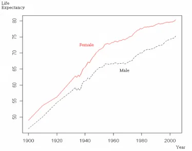
Human life expectancy has been experiencing a steady and probably the longest increase in history since the turn of the 20th century. It is believed many factors contribute to the prolonging of life, such as medical and environmental improvements. For example, the life expectancies of both U.S. males and females were less than 50 years at the beginning of the 1900s and have increased rapidly to be higher than 70 at the end of 20th century (Figure 1). The increments are about 30 years in 100 years, which is about 0.3 years annually. The trend is likely to continue, at least for a while, and the life expectancies of males and females at the end of 2008 are 75 and 81, respectively (CIA World Factbook).1 The phenomenon of prolonging of life also appears in other countries. According to the United Nations, on average, life expectancy had an increment of 0.25 years annually during the 20th century.
Figure 1. Life Expectancy in the U.S. in the 20th Century
The prolonging of life has dramatically changed individual’s life planning, especially for retirement, in the 21st century. Many believed that the life limit is 85, and some social welfare related systems and annuity products were designed according to this conjecture.
1
Recently, many countries started to feel the pressures of underestimating the scale and speed of prolonged life. Japan, known as the longest living country now, had a much shorter lifespan and did not anticipate the rapidly decreasing mortality. As a result, some insurance companies face financial insolvency. The social security system in the U.S. faces a similar problem, partly due to the elderly experiencing lower mortality than expected. According to the 2012 annual report from the Social Security Board of Trustees, the combined Trust Funds are expected to be exhausted in 2033 – three years sooner than projected in 2011. If the trend of reducing mortality continues its pace, there will be more countries facing similar problems.
Figure 2. Survival Curves of Taiwanese Females
However, because of the rapid increase in life expectancy over such a short period, there is not enough data to model the mortality rates of the elderly. There are even less data available for the oldest-old (people 85 and older) for exploring if life expectancy has a limit. Therefore, there is still no consensus about the life limit. Nonetheless, researchers believe many countries do share some common features in mortality. Rectangularization of the survival curve, or mortality compression, is one of them. According to Fries (1980), this is a state in which mortality from exogenous causes is eliminated and the remaining variability
in the age at death is caused by genetic factors. Take the survival curves in Taiwanese females as an example (Figure 2)2
In addition to describing the significant mortality reduction in premature ages, some researchers use rectangularization to measure if human life has a limit. Kannisto (2000) proposed some statistics to check if human life has a limit. He found that, although life expectancies of the U.S. and European Union countries continue to increase, more deaths occur in a shorter age interval (i.e., mortality compression). Cheung et al. (2005) proposed three-dimensional measures for the survival curve, including horizontalization, verticalization and longevity extension. They applied the data from Hong Kong and also confirmed mortality compression. However, the number of survivors
. It is obvious the mortality rates for infants and children have lessened significantly from years 1920 to 2000 (lines 1 to 9, with an increment of 10 years from numbers 1 to 9), and the survival probability for an infant to age 50 is more than 90 percent in 2000. The majority of deaths occur between ages 65 and 85, accounting for about 50 percent of deaths in 2000.
x
l and number of
deaths d used in the past studies are all from life tables, not the raw data. The numbers x
found in life tables are all graduated values and may vary a lot if choosing different graduation methods.
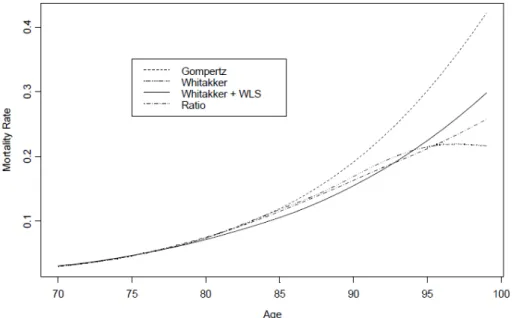
The graduation would have a larger impact on the mortality of the elderly, since there are fewer observations available. The graduated mortality rates may differ greatly, if different graduation methods or criteria are used. We shall use the 1999-2001 Complete Life Table for Taiwanese males as a demonstration. Figure 3 shows the mortality rates of ages 70 to 99, using different graduation methods. The mortality rates show obvious differences starting at age 80 and can differ almost up to 100 percent around age 99. As a result, the numbers of survivors and deaths converted from the mortality rates also have many
2
The Taiwanese complete life tables, including the survival curves and related statistics in this study, are from the Ministry of Interior, Taiwanese Government. (http://sowf.moi.gov.tw/stat/Life/List.html; data retrieved on June 15, 2012.)
differences and thus influence the measures of rectangularization. Note that, in addition to the graduation methods, the assumption of ultimate age in constructing the life tables can also affect the numbers of survivors and deaths.
Figure 3. Mortality Rates of Taiwanese Males (1999-2001 Complete Life Table)
In this paper, to avoid the influence of graduation methods, we propose using the raw data from several countries to measure rectangularization. For the rest of this manuscript, we shall first introduce the past work related to mortality compression and potential limitations of the methods used. We will describe the proposed measurements for evaluating rectangularization and show the results of empirical analysis in Section 3. We then discuss the implications of our findings on insurance in Section 4, followed by discussions and limitations of the study in Section 5.
2. Review of Mortality Compression Studies
The rectangularization of the survival curve indicates death ages are more concentrated and are with less variability (or variance). This idea was first proposed by Fries (1980). He believed that by eliminating exogenous causes of death, everyone should have about the
same life expectancy, excluding the variability from genetic factors. He also thought life expectancies were close to a limit, based on data from the U.S. and Europe. In addition, he hypothesized lifetime illness will be compressed into a shorter period before death (morbidity compression). Although some studies claimed they have proved Fries' hypotheses (Vita et al., 1998), the issues of mortality and morbidity compressions remain controversial and there are no concrete evidences.
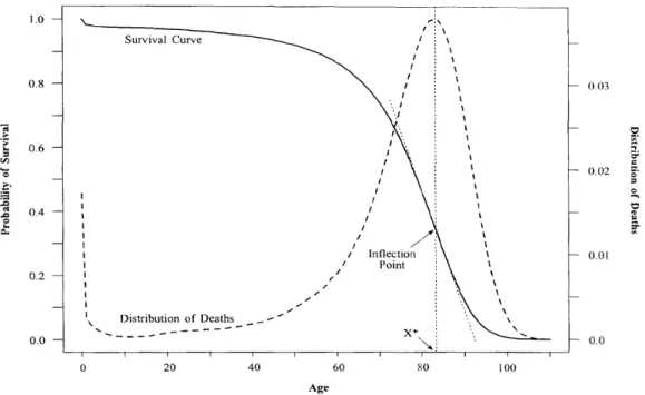
To study the compressions of mortality and morbidity, Wilmoth and Horiuchi (1999) proposed 10 measurements on the survival curves to evaluate whether the variability of deaths and illness is less. The measurements include six in quantifying rectangularity and four in computing variability. Wilmoth and Horiuchi suggested using the interquartile (IQR), or the difference of first and third quartiles, to measure if there are compressions.
Figure 4. Survival and Mortality Curves (Source: Wilmoth and Horiuchi, 1999)
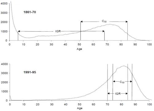
Kannisto (2000, 2001) applied the numbers of deaths from life tables and calculated the IQR and varies percentiles. He confirmed the mortality compression, using the data from 22 countries. For example, Figure 5 shows the numbers of deaths for Swedish males, from the
1861-70 and 1991-95 life tables. It is obvious that both the IQR and the smaller number of ages covering 50 percent of deaths, denoted as C50, are smaller in years 1991-95. This
indicates that the ages of deaths are becoming more condensed. Kannisto also concluded that the numbers of deaths on the right side of mode (age with highest values) do resemble the shape of a normal curve.
Figure 5. Numbers of Deaths of Swedish Males (Source: Kannisto, 2000)
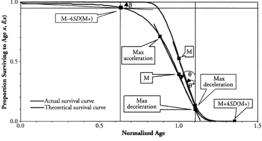
Cheung et al. (2005) modified the ideas from the previous work and proposed three-dimensional measurements for the change in survival curves: horizontalization, verticalization and longevity extension (Figure 6). The horizontalization is to measure the proportion of premature deaths, such as the percentage of deaths before age 50. It can be defined as the angle between the horizontal line and survival curve ( in Figure 6), and a smaller β indicates fewer premature deaths. The verticalization is the age with the maximum number of deaths, i.e., mode, or is to measure the descending speed at the mode ( and θ in * Figure 6). A smaller value of and θ indicates there are more deaths occurring around the * modal age (i.e., the mortality compression).
Cheung et al. used the complete life tables from 1976-2001 in Hong Kong and found the verticalization is more obvious than the horizontalization, indicating the longevity extension seems to slow down. Note that, since there is insufficient data, the mortality rates of ages 85 to 120 in Hong Kong are graduated using the logistic curve. Note that M+ in Figure 6 corresponds to changes in the right-hand tail of the survival curve and describes how far the highest normal life durations can exceed the modal age at death.
Figure 6. Three-dimensions of Mortality Compression (Source: Cheung et al., 2005)
From the brief review of the past work, we can see that the current studies of mortality compression all rely on the values of life tables. However, usually life tables are developed through a graduation process. The graduation methods and assumption (e.g., the ultimate age or the highest age attained) have noticeable influences on life table values, but the methods and assumptions are quite different depending on the users. Ideally, studying mortality compression should not depend on the choices of methods and assumptions. In the next section, we propose using the raw data, instead of the graduated values, to evaluate the mortality compression.
3. Proposed Measurements and Empirical Studies
In this section, adapting the idea from Cheung et al. (2005), we shall first introduce the modified measurements based on the raw data, instead of the graduated values. Then, the modified approach will be applied to the data from Japan, Sweden and the U.S. We shall first define the notation before introducing the proposed approach.
The number of deaths between age x and x+1 is denoted by d in life tables, which x
can be expressed as dx =lx⋅qx, where l is the number of survivors aged x, x q is the x
(conditional) probability of an individual age x who will die before age x+1. If we use the survival probability p , orx px = 1−qx, then the (unconditional) probability of an individual
age 0 who will die at ages between x and x+1 is:
∏
− = − ⋅ = ⋅ 1 0 0 (1 ) x y y x x xp q q q (1)We can also derive the number of deaths via dx =l0⋅xp0⋅qx, where l is the number of 0
survivors at age 0 (i.e., radix, usually set to be 100,000). Because l is a fixed value, the 0
new expression of d does not depend on the assumption ultimate age and the mortality x
rates of age greater than x. Then, we can still use the values of d to evaluate mortality x
compression without being influenced by graduation methods and assumptions. Note that these life table functions, i.e.,qx, px,dx,lx, are all defined in a period (not cohort) basis.
As expected, using the raw data, the age specific mortality rates q in (1) would not x
be smooth and are likely to have fluctuations, and so do the numbers of deaths d derived x
fromq . Therefore, the survival and mortality curves will not be smooth as shown in Figure x
4, and the measurements to evaluate mortality compression are not easy to define. For example, it is difficult to compute the angles of horizontalization β and verticalization θ in Cheung et al. (2005). Thus, we need to modify measurements for evaluating the mortality compression.
The mode age (denoted by M), which has the largest values of d , should be highly x
correlated with life expectancy.
The probability of premature death is defined as P(0 ≤ X ≤ m), m = 10, 20, 30, 40, 50, where X is the random variable of age-at-death. The meaning of this measurement is similar to the horizontalization.
The smallest number of ages covers the probability α of deaths, or Cα = P(x ≤ X ≤ x+δ) = α, where δ > 0. This is the same measurement used in Kannisto (2000) and it is closely linked to the verticalization.
The variance of age distribution for deaths σ . 2
The probability of survival beyond a high age, or P(X > M + kσ), where k > 0.
The first three measurements can be treated as the three-dimension measurements in Cheung et al. The last two can be used to evaluate the life limit and check if the age distribution for deaths satisfies normal distribution assumption.
It should be noted that, in addition to the usual formula for computing sample variance, there are other ways for computing the variance of age distribution for deaths. As mentioned by Kannisto (2000), the numbers of deaths on the right side of the mode do resemble the shape of the probability density function of a normal distribution. Plugging the probability density function of a normal distribution, we have
) 1 e x ) ( ) ( ) ( ) ( 1 1 2 2 2 2 2 1 2 σ − = ⋅ ⋅ × ⋅ = ⋅ + + + + + + x x x x x x x x x q p q p q p d d d . (2)
In other words, if the ratios of numbers of deaths in (2) are not constant of age, then the assertion by Kannisto is not true. If the ratios are fixed, then the weighted least squares can be used to compute the variance, after taking the logarithm on both sides of (2).
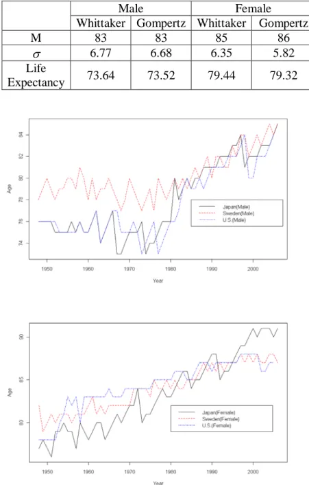
Before showing the empirical results of data from Japan, Sweden and the U.S., we first compute the proposed measurements under two graduation methods. Table 1 shows the results based on 1999-2001 Taiwan data. We can see that using different graduation methods
of the standard deviation σ estimate has a larger difference for the female data, and the difference in σ estimate is about 9 percent. Suppose the same data set is used. We would still observe differences if different graduation methods are used, which indicates the potential problems for using the graduated values.
Table 1. Two Graduation Methods in Taiwan 1999-2001
Male Female
Whittaker Gompertz Whittaker Gompertz
M 83 83 85 86
σ 6.77 6.68 6.35 5.82
Life
Expectancy 73.64 73.52 79.44 79.32
The mortality data of Japan, Sweden and the U.S. are all from the Human Mortality Database (HMD). The data periods of these three countries are different, according to the data availability, where Japan is 1947-2006, Sweden is 1901-2007, and the U.S. is 1933-2005. To compare these three countries, only the time period 1947-2006 is used. We will first discuss the mode ages with the largest values of d for these three countries x
(Figure 7). The modes of males are near constant before the 1980s and increase linearly after that. Also, the modes of Sweden are obviously larger before 1980 and now the three countries have about the same mode ages. The modes for females show a similar pattern but their increments are more stable. Japanese females appear to have larger modes than those in Sweden and the U.S. Heuristically speaking, the mode can be treated as life expectancy and the trend of the mode indicates that the human life continues to extend.
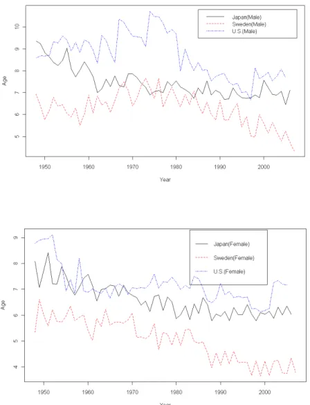
Figure 9. The Shortest Age Intervals of 25 Percent, 50 Percent and 75 Percent
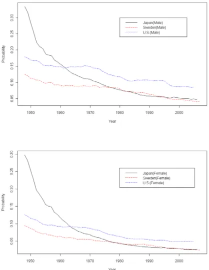
The ideas similar to the horizontalization and verticalization in Chueng et al. (2005), i.e., the probability of premature death and the smallest number of ages covers the probability of deaths, are shown in Figures 8 and 9. Figure 8 shows the probabilities of dying before age 50. The probabilities of death of Japanese males and females are more than 0.30 in the 1950, the highest among three countries, and have the largest decreasing rates. The probabilities of death in Sweden and the U.S. seem to decrease constantly, and the differences between these two countries are about 5 percent. The probabilities of death of Japan and Sweden are about the same since 1980. Also, the probability of death in the U.S. is the largest after 1970,
and this is highly correlated to the shortest life expectancy. Figure 9 is the smallest number of ages covering certain probabilities of deaths, and this is similar to the idea of verticalization. No matter if the probability is 25 percent, 50 percent or 75 percent, the age ranges tend to decrease gradually. This indicates that the distribution of deaths is more concentrated, which seems to support the mortality compression. Also, the age ranges of the U.S. are the widest among the three countries.
Figure 10. The Standard Deviations of Death Age
Based on the preceding measurements, life expectancy seems to extend gradually and the mortality compression tends to hold. The standard deviation of age distribution for
deaths will be used as a double check for the mortality compression. However, instead of following the method of Cheung et al. (2005), we use raw data and apply the weighted least squares on (2) to compute the variance. Note that, the differences are less than 10 percent if applying the method of Cheung et al. Figure 10 shows the standard deviations and there exist noticeably large fluctuations since the raw data are used. But unlike the result of Hong Kong in Cheung et al., the standard deviations do not always decrease. Those of Japan and the U.S. seem to level off, while those of Sweden do decrease annually. We do not have concrete evidence for supporting the mortality compression.
The probabilities of surviving beyond very high age do not support the mortality compression either. Figure 11 shows the survival probabilities beyond the mode plus one standard deviation and two deviations of age distribution. The ages of these two bounds are approximately 95 and 100, and thus can be treated as “very high age” survival probability. (It is like the elderly of age beyond 85 defined as “oldest-old.”) We can use these two survival probabilities as proof of whether life extension reaches a limit. Because of the insufficient sample of the elderly, the survival probabilities have larger fluctuations (about 40 percent more). Interestingly, the survival probabilities of the three countries are very close to each other. In general, the survival probabilities beyond M+ of males and females are about 10~12 percent and 11~13 percent, respectively, and those beyond M+2 of both males and females are about 1~2 percent.
Although the measurements of horizontalization and verticalization support mortality compression, the standard deviation and the survival probability beyond very high age provide another possibility for future life expectancy. In particular, the survival probabilities beyond very high age and the standard deviations of age distribution for Japan and the U.S. all look constant. Together with if the mode age (or life expectancy) continues to increase, it seems that life expectancy having a limit is still an open question. We tend to believe life is without a limit, where the survival curve is likely to move to the right, as shown in Figure 12.
Figure 11. The Probability of Survival Beyond a High Age
4. Implications to Annuity Products
The continuing reduction in mortality rates has been creating difficulties in designing annuity products. In the past, people tended to believe that life expectancy would stay constant or reach a limit. For example, in the 1960s, the consensus was that human beings would likely not live beyond age 85. However, just after 40 years, the life expectancies of some countries have already surpassed 85 years, such as happened in Japan and Hong Kong in 2007. The assertion that life expectancy is a constant or has a limit now is questioned by many researchers.
Instead, it seems life expectancy is more likely to continue increasing, at least for the near future. To address the increasing life expectancy, stochastic mortality models have become a popular tool in calculating the value of annuity products. The Lee-Carter model (Lee and Carter, 1992) and the reduction factor model (Continuous Mortality Investigation, 1999) are two of the famous mortality models. Life expectancy under these models also will continue to increase. Unlike the previous studies, we used the raw data to verify mortality compression and found there are no obvious signs of converging life expectancy. On the contrary, the results support that life expectancy is going to extend, like in the stochastic models.
Although it is assumed that life expectancy would extend in the stochastic models, there are still doubts for using them to model annuity products. For example, in the Lee-Carter model, where the age-specific mortality rates are assumed to reduce exponentially annually, the reduction rate plays an important role in pricing. If the reduction rate is underestimated, the annuity products will be underpriced. However, there are insufficient data of the elderly, and this raises doubts in estimating reduction rates for the elderly, especially for the oldest-old. Because there are insufficient samples for people 90 and older, modeling
mortality rates of the elderly usually relies on extrapolation methods, such as the Gompertz law. This means we are not sure about the right tail of the survival distribution and depend solely on assumptions to price annuity products. Thus, it is difficult to evaluate the risk of using stochastic mortality models to price the annuity products.
If the mortality compression is true, we can use it to modify mortality models and evaluate the risk. Unfortunately, we found that mortality compression is not always true. If the variance (i.e., risk) of the death age distribution is decreasing, we have more confidence in designing annuity products. But, from the historical data from Japan and the U.S., the standard deviations seem to be constants. Besides, the survival probabilities beyond ages 95 and 100 (approximately, M+σ and M+2σ) also behave like constants. This indicates there is a non-negligible probability for the right tail of the survival distribution that is still unknown or without enough observations.
In other words, the study of mortality compression does not help to relieve doubts in using the mortality models. Instead, the results in this study might lead to another possibility in designing annuity products. For example, since the survival probability beyond M+2σ is about 2 percent, this suggests that the death age distribution is well studied on the left hand side of M+σ (or even M+2σ). But, for the age distribution beyond M+2σ, fewer data are available and it is difficult to evaluate the survival probability, especially to predict the future survival probability.
One of the possible approaches for dealing with longevity risk is to concentrate on the part with more confidence. For example, we can focus more on products like annuity-certain, and design the annuity payable up to the age of M+2σ and consider other tools to cope with ages beyond M+2σ. Note that the age of M+2σ is about 100 years old and there is about 2 percent of probability of surviving beyond this age. It would be plenty for most people.
There are several ways to tackle the coverage of survival beyond the age M+2σ, but first we need to decide the role of annuity products in planning one’s retirement life. If the
annuity products are not the primary source of income, then the coverage up to the age
M+2σ probably is enough. If the insured relies solely on annuity products, then we need to
deal with estimating the probability of surviving beyond age M+2σ. However, up to today, there is not enough data to estimate this probability.
5. Discussions
Since the idea of mortality compression and rectangularization was proposed in 1980, many studies have tried to verify the idea and check if it can be linked to exploring the theory of life limit. Although it is believed that life expectancy will increase in the future, the theory that there is a limiting age to life is preferred. However, in verifying the mortality compression, most studies use graduated mortality rates from life tables instead of the raw data. Of course, the graduated values usually are very smooth, and it is easy to capture properties of survival curves by visualization. But the graduation might distort the nature of mortality rates. Since the numbers of observations for the elderly are seldom sufficient, their graduated mortality rates are likely to be very different from the true values and cause false decisions. The data problem of the elderly possibly is the most challenging for the study of human longevity.
The problem is even more obvious if the focus is on areas with few populations. For example, Cheung et al. (2005) studied mortality compression in Hong Kong, based on the whole life tables, where three-year death records are used. However, as shown in our study, techniques of constructing life tables may have significant influences on mortality rates and possibly on the conclusion of mortality compression. Thus, we propose measurements to evaluate mortality compression based on raw data to reduce the influence of graduation. Still, insufficient samples of the elderly cause fluctuations in the measurements, which are especially observable in the case of Sweden since it has the smallest population.
as in Cheung et al. We found the age with the largest number of deaths (mode M) increases annually, and the probability of premature death (horizontalization) and the smallest number of ages covers the probability of deaths (verticalization) decrease annually. But for the issue of whether life expectancy has a limit or mortality compression, our findings are not the same as that in Cheung et al. The standard deviations of the death age distribution show different patterns. Like in Hong Kong, the standard deviations in Sweden seem to decrease gradually but those in Japan and the U.S. look like constants, which means there are inconclusive evidences for supporting the mortality compression and the theory of life with a limit.
In addition, we found the probabilities for surviving beyond the age of M+σ or M+2σ (i.e., very high age) remain constants in the three countries and both sexes. This can be used to act against the theory that life expectancy is reaching a limit. Note that, although the standard deviations show different patterns, the sum of the mode age and standard deviation also increases (like the mode M). Together with the result that the probability of survival beyond a very high age is constant, it seems life expectancy will continue to increase. Li et al. (2008) also had a similar conclusion. They proposed a model using the idea from extreme value theory and found that the human lifespan is not approaching a limit, based on the raw data from the HMD.
The prolonging of life has increased the complexity of designing annuity products and the insufficient data of the elderly even makes the situation more complicated. The lack of data escalates the risk in designing annuity products, due to the variances of mortality estimates. The findings in this study might provide some possible alternatives for the problem. For example, we can use the result that the probability of survival beyond very high age is close to a constant, to reduce the risk to annuity products. A possible approach is to design annuity-certain products and let the annuity be payable up to a very high age (e.g.,
very high age (about 2 percent of probability).
Our study wants to show that the data quality is crucial in exploring the mortality compression. Most of the previous work used graduated data (e.g., mortality rates and death numbers) from life tables. These numbers follow the assumption of stationary population, with same radixl0 =100,000,meaning that 100,000 newborns every year. The proposed method intends to avoid the stationary population assumption and to use the population size to adjust the estimation (weighted least squares). Note that all countries involved in this study, official population counts are available at least up to age 90 (Jdanov et al, 2008). The HMD makes adjustment for the mortality rates over age 90 by the survivor ratio method (Thatcher et al, 2002). Since the population over age 90 is not much, the adjustment has a small impact on the estimation of modal age and standard deviation σ (Yue, 2002).
The results we found are for Japan, Sweden and the U.S., and it does not mean they will apply to other countries. There are reasons for choosing these three countries as a pilot study. These countries have larger populations, longer life expectancies, and especially good data quality and longer data periods. We applied the proposed measurements to Taiwan data and found some funny results that are not easy to interpret. For example, the standard deviations of the death age distribution are decreasing but the probabilities for surviving beyond the age of M+σ or M+2σ are increasing. We will continue exploring the mortality compression on other countries.
In this paper, we proposed measurements based on the raw data to evaluate the mortality compression, to reduce the influence of graduation in life tables. However, since the values are not graduated, the results generally are not very smooth and fluctuate a lot. The fluctuations are particularly obvious for the case of Sweden and would also be for areas with small populations. We can combine the single-year results to smooth the measurements (such as a three-year or a five-year moving average). But for areas with populations less than in Sweden (e.g., Hong Kong), measurements from the single-year data still will be not
good enough and multi-year data might be needed. If this is the case, then the proposed measurements need to be modified.
References
Cheung, S.L.K., Robine, J., Tu, E.J., and Caselli, G. (2005) “Three Dimensions of the Survival Curve: Horizontalization, Verticalization, and Longevity Extension Source.” Demography, Vol. 42(2), 243-258.
Continuous Mortality Investigation Report No. 17(1999), Institute of Actuaries and Faculty of Actuaries.
Fries, J.F. (1980) “Aging, Natural Death, and the Compression of Morbidity.” New England Journal of Medicine, Vol. 303(3), 130-135.
Jdanov, D.A., Jasilionis, D., Soroko, E.L., Rau, R., Vaupel, J.W. (2008). “Beyond the Kannisto-Thatcher Database on Old Age Mortality: An Assessment of Data Quality at Advanced Ages.” MPIDR Working Paper WP-2008-15. Rostock: Max Planck Institute for Demographic Research.
Kannisto, V. (2000) “Measuring the Compression of Mortality.” Demographic Research, Vol. 3, Article 6. (www.demographic-research.org/Volumes/Vol3/6)
Kannisto, V. (2001) “Mode and Dispersion of the Length of Life.” Population: An English Selection, Vol. 13, 159-171.
Lee, R.D., Carter, L. R. (1992). “Modeling and forecasting U.S. mortality.” Journal of the American Statistical Association, Vol. 87 (419), 659-675.
Li, J.S.H., Hardy, M.R., and Tan, K.S. (2008). “Threshold life tables and their applications.” North American Actuarial Journal, Vol. 12, 99-115.
Thatcher, A.R., Kannisto, V. and Andreev, K. (2002). “The survivor ratio method for estimating numbers at high ages.” Demographic Research, Vol. 6(1):2-15.
Vita, A.J.; Terry, R.B.; Hubert, H.B.; Fries, J.F. (1998), “Aging, health risks, and cumulative disability.” New England Journal of Medicine, Vol. 338, 1035–1041.
Wilmoth, J.R. and Horiuchi, S. (1999) “Rectangularization Revisited: Variability of Ageat Death within Human Populations.” Demography, Vol. 36(4), 475-495.
Yue, C. J. (2002). “Oldest-Old Mortality Rates and the Gompertz Law: A Theoretical andEmpirical Study Based on Four Countries.” Journal of Population Studies, Vol. 24, 33-57.出席國際學術會議心得報告
計畫編號 99-2410-H-004 -064 -MY2 計畫名稱 死亡壓縮及死亡模型在延壽風險的應用 出國人員姓名 服務機關及職稱 余清祥(國立政治大學統計系教授) 會議時間地點 2011 年 9 月 8 日~9 日會議名稱 Longevity 7: Sixth International Longevity Risk and Capital Markets Solutions Conference
發表論文題目 Modeling Mortality for Countries with Small Populations
一、參加會議經過
國際 長壽 風險研 討會(International Longevity Risk and Capital Markets Solutions Conference)已經是第七屆,主旨在於探討壽命延長對保險業造成的影響,參加研討會的 成員範圍愈來愈廣,不再以學校及研究機構的學者為主,與會來賓許多來自各大保險公 司及政府機關,顯示長壽議題愈受重視。以本次會議所在的歐洲為例,近幾年因為壽命 延長的影響增大,歐盟 30 個國家中已有 13 個國家,將原有的固定給付(Defined Benefit) 全部、或部份修改為固定提撥(Defined Contribution),政府不再全部承擔壽命延長而增加 的費用。臺灣自從 1993 年 65 歲以上人口比例突破 7%,達到聯合國定義高齡化社會的標 準,這個比例急遽上升,在 2010 年底超過 10%,甚至在 2030 年超越 20%(2010 年行政 院經建會人口推估),這個人口老化速度堪稱世界之最,國人即將面對長壽風險(Longevity Risk)帶來的衝擊。長壽風險和本人研究的死亡率理論、生態平衡有關,近年來除了延續 在這些領域的理論研究,為了增加統計應用及影響,也與保險實務結合,和保險、財務 領域學者合作,共同為解決因為人口老化(Population Aging)引起的問題而努力。 二、與會心得 本次(第七屆)國際長壽風險研討會在德國法蘭克福市舉辦(歌德大學財務學院, 如照片),法蘭克福的九月有點微寒,穿著長袖衣物剛好,可惜會議期間陰天微雨,無法 享受德國多樹的街道,搭配藍天、白雲、秋風的那份舒適。今年研討會中發表的論文較 去年更為多樣化,包括以往的世代生命表(Cohort Life Table)、動態死亡率模型(Dynamic Mortality Models)等主題,也有不少文章探討長壽風險的影響及應對措施,希冀對政府及
特性的國家,提高死亡率估計及預測的準確性。 除了和各國學者交換研究心得外,本次有較多機會和各國保險業者、政府官員聊天, 瞭解各國面對長壽風險的態度。其中從德國保險公司的與會者得知,德國二十年前年金 險商品的總保費,比例不到所有人壽保險商品的 20%,但今日已達到 80%,顯示生存型 商品因為壽命延長而角色日漸吃重,這個現象和美國、日本類似。年金險在今天的臺灣 壽險商品市佔率和德國二十年前類似,大約不足 10%,未來少子化、人口老化將改變國 人退休後的經濟來源,預計年金商品將大幅增加,但國內保險業者的準備明顯不足,對 壽險業經營形成潛在危機,政府及保險業者需要積極面對。
Modeling Mortality for Countries with Small Populations
Hong-Chih Huang1, Jack C. Yue2, and Hui-Ting Wang3
Abstract
The prolonging longevity is a common phenomenon in the 21st century and it becomes important and necessary to forecast the mortality rates for the elderly. However, the data available for the elderly usually are very limited, with respect to the sample size and period. The small sample size, especially for a country with few populations, incurs high volatility in mortality and finding a good mortality model would be more challenging. In this study, we propose a method for reducing the volatility in small countries, by taking advantage of other countries’ mortality data with similar mortality experience. First of all, we adopt cluster analysis to select countries with similar mortality profiles as the target country. Next, we apply the principle component analysis for the selected countries and use the data reduction skills to reduce the mortality volatility for the small country. We use the mortality data from the human mortality database (data period: 1970–2008) to evaluate the proposed method, and the proposed PCA model produces significant smaller prediction errors than the Lee-Carter model for almost all illustrated countries. We also use the proposed mortality model in pricing and valuation for Taiwan data.
Keywords: Cluster Analysis; Longevity Risk; Small Area Estimation; Principle Component Analysis; Data Reduction
1
1.
Introduction
Human life expectancy has been increasing significantly since the start of the 20th century, though increments of life expectancy vary with countries and genders. For example, in most Western countries, life expectancies at birth were approximately 66 and 70 years for men and women in 1950, and then surpassed 75 and 80 years by 2005 respectively. In Asia, life expectancies were much lower at the turn of 20th century, but the mortality improvement has been much faster and greater and the life expectancies of many Asian countries are about the same as those of Western countries. For example, the life expectancies in 2005 are 79 and 86 years for Japan male and female, and they are approximately 75 and 81 years for Taiwan male and female.
In the past two decades, a wide range of mortality models have been proposed to model the unprecedented life longevity in history. Among them, the Lee-Carter (1992) or LC model is probably the most popular choice, because it is easy to implement and outperforms many models with respect to its prediction errors (e.g., Koissi et al., 2006; Melnikov and Romaniuk, 2006). Various modifications of the LC model offer broader interpretations (Brouhns et al., 2002; Renshaw and Haberman, 2003), and many countries continue to use the LC model as the base mortality model for their population projections. For example, the Continuous Mortality Investigation Bureau (CMIB, 2006) in Britain suggested the LC model as a means to compute stochastic mortality rather than the reduction factor model that it previously proposed.
Because many empirical studies showed that the LC model has room for improvement, a lot of modifications have been proposed. For example, it is found that the age parameters (α andx β ) x
are not time-invariant, especially for older age groups (Carter and Prskawetz, 2001; Huang et al., 2008). Among all modifications, adding a cohort effect (Renshaw and Haberman, 2006; Cairns et al., 2007) or another period effect (Yang et al., 2010) is one of the popular choice.
The original estimation of the LC parameters does not involve weight adjustment, and this would create fluctuations in estimates if the populations are small. Recently, there is a growing need to model the mortality rates of small populations and many suggest using information from larger populations to improve the estimation of smaller populations. For example, Li and Lee (2005)
proposed a coherent approach, by fitting the joint trend of LC model with a larger population (i.e., a group of smaller populations) and still keeping some specificity of smaller populations. Njenga and Sherris (2009) co-integrate various countries’ mortality data and apply the vector error-correction model (VECM) and principal component analysis to build a model for larger population. Cairns et al. (2010) applied Bayesian method to connect the mortality data of both a large and small areas.
In this study, we are also interested in mortality models for small populations. In particular, our goal is to improve the mortality estimation and prediction of a small population, provided that there are mortality data from other populations. We want to know the way for choosing populations which have similar mortality properties as the target population. We shall use the techniques of cluster analysis to select similar populations and the principal component analysis for data reduction.
For the rest of this paper, we shall introduce the proposed approach in Section 2, including the idea of applying cluster analysis and principal component analysis. In Section 3, we evaluate the approached method using the mortality data from Human Mortality Database and then compare the fitting results with the LC model. In addition, we apply the method to Taiwan experience data in Section 4, and then conclude with discussions and limitations of our approach.
2. The Proposed Approach
Since the variance (or volatility) is in inverse proportion to the sample size, the parameter estimation in smaller populations usually has a larger fluctuation. To increase the sample size is a natural choice for lower the fluctuation, and it is assumed that there is a larger reference population in the previous work. In this study, however, suppose there are a target (small) population and a lot of populations available. The goal is to find populations which have similar mortality experience as the target population, and combine these populations in order to acquire more reliable estimation.
For example, suppose we want to model Taiwan’s mortality rates, using the mortality data from the HMD4
“similar mortality experience” and a possible choice is to check whether two populations have similar mortality improvements at all ages (more general than identical mortality rates at all ages). In other words, we first compute the mortality improvement at all ages, or rx(t)=qx(t+1)/qx(t), whereqx(t)is the age-specific mortality rate of age x at time t. Next, we shall check if two populations share similar behavior inrx(t) for all ages, and we adopt the cluster analysis to select countries that have similar mortality experience as Taiwan. Finally, we combine the data of these countries, together with Taiwan data, and apply the principal component analysis to model mortality rates.
In the following discussions, we shall briefly describe the processes of cluster analysis and principal component analysis used in this study.
Choosing Countries using Cluster Analysis
The cluster analysis (CA) is to classify a set of observations/variables into one, two, or more mutually exclusive groups, and the observations/variables within a group share properties in common (i.e., homogeneity). It is cognitively easier to model and predict a homogeneous group, rather than a heterogeneous group. Heuristically speaking, if two countries have similar mortality improvement at all ages, the differences of rx(t) at all ages shall be very close. In other words, applying the CA to the differences of rx(t), there shall be only one cluster. If there are two or more than two clusters, this indicates that not all ages have similar mortality improvement rates and these two populations do not have similar mortality experience.
The distance measure plays an important role in deciding the number of clusters in the CA. Among possible choices of distance measure, we choose the Euclidean distance, due to its popularity. In the beginning, each individual (observation or variable) is treated as a cluster (or group) and then individuals are merged into a cluster according to their distances, until meeting certain criteria. Basically, the final grouping is a balance of two criteria: minimizing the average distance within clusters and maximizing the distance between clusters. Usually, we can apply the AIC (Akaike Information Criterion) or BIC (Bayesian Information Criterion, or Schwarz’s Criterion) to decide the optimal number of clusters. The AIC & BIC are designed to avoid the possibility of
over-parameterization, which takes the fitting errors and the number of parameters into account. The AIC & BIC are defined as
( )
(ˆ) log 2 2ν l φ AIC= − (2.1) and( )
l nBIC=−2log (φˆ) +νlog , (2.2)
where ( )l φ
∧
is the maximum estimate of likelihood function, v is the number of parameters being estimated, and n is the number of observations. The smaller the AIC/BIC is, the better the model fit is.
Note that there are several ways to define distance within a cluster and distance between clusters. Usually, the average distance (or Average Linkage) and the Ward’s minimum variance criterion are the most popular choice of distance. The average distance within a cluster is to measure the average distance of all individuals to cluster center, and the distance between clusters are the Euclidean distance between two cluster centers. The Ward’s criterion is defined similarly, except the calculation of distance is replaced by the variance. In this study, we choose the Ward’s minimum variance criterion.
We will use the mortality data (age-specific mortality improvement of single age, 1970-2000) from Taiwan and U.S. to demonstrate the optimal number of clusters. The variables used are the mortality improvement of each age (ages 0-99) in Taiwan and U.S. and Table 3-1 shows the information of AIC and BIC for all possible numbers of clusters. In principle, the smaller the AIC & BIC is, the better the choice is. For example, the optimal number of clusters is 6 judging via the AIC, and 2 via the BIC. Because the AIC and BIC usually have different choices, sometimes we calculate the ratio of distance for the current number of clusters to one less number of clusters (Ratio of distance measure on Table 2-1). A larger value of the ratio of distance indicates a larger distance between clusters, a preferred result. In this study, we will use the AIC as the primary criterion, and fewer clusters are preferred. Thus, it seems 3 clusters is a feasible choice and this suggests that the mortality experiences of Taiwan and U.S. are not very similar.
Table 2-1. Optimal Number of Clusters for Mortality Similarity between Taiwan & U.S. # of Cluster AIC BIC Ratio of distance
measure 1 2131.692 2283.369 --- 2 1925.121 2228.475 1.580 3 1822.094 2277.125 1.750 4 1774.748 2381.456 1.070 5 1873.571 2631.956 1.303 6 1529.755 2439.817 1.089 7 1627.571 2689.310 1.229 8 1722.177 2935.593 1.082 9 1790.095 3155.188 1.073 10 1895.513 3412.282 .939
Using the Principal Component Analysis for Mortality Estimation
After deciding the countries that share similar mortality experience as the target population, we will use all the data from these countries to model mortality rates. Since there are a lot of variables, we need to apply techniques of data reduction before modeling the mortality. Similar to Yang et al. (2010), we choose the principal component analysis (PCA) since the PCA is easy to use. Singular value decomposition (SVD), used in estimating the parameters of the LC model, is another possible choice for data reduction. Since the SVD and PCA usually give very similar results, we will consider the PCA only in this study. The functional PCA approach by Hyndman and Ullah (2005) is also a possible choice.
The PCA is a popular analysis method for dealing with multivariate data, and it can be used for data reduction and interpretation. As the dimension (i.e., number of variables) of data increases, summarizing the data would become more difficult. The PCA is to find uncorrelated components (as fewer components as possible) but still preserves the data properties. Note that the components extracted are linear combinations of original variables. The PCA is derived based on the covariance or correlation matrix (Johnson and Wichern, 2002) and its eigen-decomposition.
Similar to most of the mortality studies, the logarithms of mortality rates, instead of the mortality rates, will be used. We shall apply the PCA to the logarithms of age-specific mortality rates from countries which have similar mortality experience as the target population. Also, the
number of PC’s chosen can provide possible interpretations for the mortality rates, and the number is usually 1, 2, or 3 (Bell, 1997). For example, the LC model can be treated as an 1-PC model and the logarithms of central death rates of all age groups decrease linearly. The model proposed by Yang et al. (2010) is an example of 2-PC model, and the decreasing trends of logarithm of central death rates vary at two different time periods. The model by Heligman and Pollard (1980) can be treated as a 3-PC model, where they separate the human life into 3 different periods: infant & childhood, younger adult, and adult.
3. Empirical Study
In this section, we use the empirical data to evaluate the proposed method of obtaining more reliable mortality estimates for small populations. We shall evaluate the performance of the proposed method via cross-validation, i.e., computing in-sample and out-sample errors, using the LC model as the reference. The target population is Taiwan and the reference populations are countries (30 countries) in HMD. The data in the period 1970~1999 are used as training data, and the period after year 2000 are the testing data.
Before showing the details of empirical study, we shall first introduce the evaluation criterion. We use two criteria for evaluation and the first criterion is the mean absolute percentage error (MAPE), defined as 1 ˆ 1 100% n i i i i Y Y MAPE n = Y − =
∑
× , (3.1)where Y and i Yˆi are the actual values and estimated (or predicted) values of mortality
5
Note that we can also use the AIC/BIC to evaluate the model fit. However, the proposed , and n is the number of observations. MAPE can be used to evaluate the performances of training and testing data, and the smaller MAPE is preferred.
5
approach is to combine different countries of data, but the goal is to improve mortality estimation of a small population. In other words, the likelihood function in (2.1) and (2.2) is for multiple countries of data but the MAPE is calculated for certain population. It would be misleading if we compare the values of MAPE with AIC/BIC. Still, we will use the AIC/BIC as a reference.
Next, we will show the CA results for the 30 countries (Table I-1 in the Appendix) from the HMD, and we will first give a brief description of Taiwan population. The population in Taiwan is about twenty-three million in 2011 and Taiwan is experiencing rapid population aging. The population of age 85 and beyond was around 20,000 in 1980, surpassed 200,000 in 2010, and is expected to be more than 500,000 before 2025. Still, there are not enough of data to model the mortality rates for the elderly, and it seems that Taiwan is a good example of small population to practice the proposed approach.
Similar to the process in Table 2-1, we apply the CA to the 30 countries from the HMD (1970-1999). Table 3-1 shows the numbers of clusters if the mortality rates of single age (ages 0-99) are used. There are five countries which have similar mortality improvement as Taiwan, and they are Austria, France, Ireland, Norway, and Spain. The populations of these five countries are between four to sixty-five million, and the total 156 million, about 7 times of the population in Taiwan. Note that the CA can also be used on the mortality rates of five-age groups. However, since there are only 20 groups of 5-age mortality rates (e.g., 0-4, 5-9, …, etc), the number of clusters are almost 1 for every country. Therefore, we shall use the mortality rates of single age for CA.
Table 3-1. Cluster analysis of mortality improvement for single age (1970-1999)
Country Cluster # Country Cluster # Country Cluster #
Australia 2 France 1 Poland 1
Austria 1 Hungary 2 Portugal 2
Belarus 3 Ireland 1 Russia 2
Belgium 2 Italy 2 Slovakia 2
Bulgaria 2 Japan 2 Spain 1
Canada 2 Latvia 2 Sweden 3
Czech Republic 2 Lithuania 3 Switzerland 3
Denmark 2 Netherlands 2 UK 2
Estonia 2 New Zealand 2 USA 3
We will use the mortality data of Taiwan and 5 countries, sharing similar mortality experience with Taiwan, to model mortality rates and compare the results with those using the LC model. The comparison can be separated into two parts (Table 3-2): in-sample (or fitting period, 1970-1999) and out-sample (or testing data, 2000-2008). The mortality data appear in the format of 5-age groups, ranging from 0 to 99 year-old, for both the male and female.
Table 3-2. Data Periods for six selected countries Countries Fitting period Prediction period
Austria 1970~1999 2000~2008 France 1970~1999 2000~2007 Ireland 1970~1999 2000~2006 Norway 1970~1999 2000~2007 Spain 1970~1999 2000~2006 Taiwan 1970~1999 2000~2008
Since there are mortality rates of 5-age groups from multiple countries, we will use the PCA to reduce data dimension. Also, similar to the past studies, the mortality rates shall be taken into the form of logarithm. The key parameter in the PCA is to choose the number of principal components (PC) and there are some suggestions. One of the popular choices is to choose the PC’s with eigen-value larger than 1. Or, similarly, we can use the scree plot to see if there is obvious drop in the eigen-values. Another possibility is to look at the cumulative variation, or cumulative eigen-values to the sum of all eigen-values.
Table 3-3 shows the summary of PCA according to the eigen-value and the cumulative variation. Adapting the criterion of eigen-value larger than 1, the numbers of PC’s are 3 and 2 for the male and female, respectively. This result coincides with Bell (1997) and he suggested using 2 or 3 PC’s if applying the PCA for mortality rates. On the other hands, if we set up the cumulative variation to be 95%, then we need 7 PC’s for the male and six PC’s for the female. In the following discussion, we shall compare the performance of mortality estimation of PCA to that of the LC model, and we shall first show the result of fitting errors.
Table 3-3. Results of PCA for Taiwan male and female Male Female PC# Eigen-value Cumulative Variation (%) Eigen-value Cumulative Variation (%) 1 11.399 56.996 14.324 71.619 2 4.681 80.402 2.730 85.271 3 1.323 87.016 .889 89.714 4 .632 90.177 .628 92.855 5 .477 92.564 .341 94.559 6 .417 94.651 .224 95.679 7 .287 96.085 .199 96.673 8 .184 97.004 .155 97.445 9 .118 97.597 .112 98.003 10 .108 98.137 .097 98.489
Although the proposed method is designed to increase the fitting accuracy of Taiwan mortality rates, we can also use the PCA for the combined data to evaluate the fitting accuracy of Austria, France, Ireland, Norway, and Spain. Tables 3.4 (male) and 3.5 (female) are the fitting errors (MAPE) of the proposed method for six countries, using the MAPE’s of LC model as the reference group. The proposed model has smaller fitting errors than the LC model when five or more PC’s are used. These results are similar to those in Njenga and Sherris (2009), where as many as eight components are used to model multi-countries mortality.
Table 3-4. Fitting MAPE of the male for six countries (unit:%) # of Principal Component LC Country 1 2 3 4 5 6 7 Austria 8.91 8.95 5.73 5.38 4.43 4.00 3.56 4.38 France 9.71 6.89 4.61 4.23 3.72 2.76 2.66 3.81 Ireland 17.20 8.39 8.23 6.27 6.00 5.10 4.48 6.51 Norway 9.62 7.25 6.65 5.83 5.34 4.56 4.43 5.52 Spain 9.62 7.60 6.51 5.82 4.57 4.07 3.117 6.41 Taiwan 14.11 8.25 7.51 6.77 5.89 4.30 3.41 5.75 Total 11.53 7.89 6.54 5.72 4.99 4.13 3.62 5.40
Table 3-5. Fitting MAPE of the female for six countries (unit:%) # of Principal Component LC Country 1 2 3 4 5 6 7 Austria 8.76 7.95 5.95 4.88 4.53 4.36 3.71 4.75 France 11.68 5.75 5.07 3.65 2.88 2.15 2.03 2.85 Ireland 16.05 9.12 7.50 7.20 6.12 5.43 4.85 7.06
Spain 9.19 7.93 7.02 4.12 3.59 2.81 2.54 4.75 Taiwan 9.47 7.52 5.78 5.34 4.14 3.74 3.33 4.46 Total 10.90 7.73 6.46 5.27 4.54 4.00 3.58 5.11
We also calculate the AIC and BIC of the proposed method and compare with those of the LC model. However, since the proposed approach is for the combined data, it would be difficult to count the number of parameters in the calculation of AIC/BIC. Therefore, we plug into all parameters of the PCA to compute the AIC/BIC in Taiwan. Similarly, we also plug all parameters of the LC model used in six countries for the AIC/BIC. Table 3-5 lists the values of AIC and BIC, and it seems that fewer PC is better. Because the calculation of AIC/BIC is questionable, we will not use the results in Table 3-6 to choose PC’s.
Table 3-6. AIC and BIC of fitting results for Taiwan # of Principal Component LC 1 2 3 4 5 6 7 Parameter 66 92 118 144 170 196 222 246 Male AIC 30,107 32,572 35,565 36,103 37,755 37,828 43,098 33,394 BIC 29,698 32,003 34,835 35,212 36,703 36,615 41,724 31,872 Female AIC 33,842 35,818 38,918 40,897 41,089 42,053 46,407 36,634 BIC 33,433 35,249 38,188 40,006 40,037 40,840 45,033 35,112
Next, via the prediction MAPE, we compare the proposed method with the LC model. Time series methods (i.e., ARIMA model) are used to model the trend of future mortality. For the MAPE of predicting Taiwan mortality rates, the proposed method outperforms the LC model if the number of PC’s is two or more (Tables 3-7 & 3-8), with a reduction around 3% in MAPE. Similarly, on average, the proposed method also has smaller prediction MAPE if there are 3 or more PC’s. The proposed method has the larger reduction than the LC model for the Spain data (for both the male and female).
Table 3-7. MAPE values of forecasting results for males of six countries (unit:%) # of Principal Component LC Country 1 2 3 4 5 6 7 Austria 10.48 9.99 9.58 8.94 7.62 7.81 8.85 9.55 France 14.27 13.58 12.76 10.31 9.29 8.15 8.29 11.61 Ireland 23.25 21.82 21.12 19.02 20.09 21.22 21.29 22.72
Spain 10.57 9.79 9.77 8.62 8.75 8.66 9.13 14.04 Taiwan 22.26 15.10 15.70 15.13 14.75 14.90 14.86 18.13 Total 15.73 13.93 13.71 12.54 12.23 12.22 12.40 14.72
Table 3-8. MAPE values of forecasting results for females of six countries (unit:%) # of Principal Component LC Country 1 2 3 4 5 6 7 Austria 13.03 11.77 11.88 10.33 10.12 9.74 9.67 10.88 France 13.67 14.34 13.34 10.63 8.26 7.54 7.64 10.03 Ireland 16.06 14.34 14.35 14.74 13.93 14.00 13.70 15.50 Norway 14.95 14.97 15.59 13.86 12.96 12.93 13.70 14.58 Spain 7.07 6.58 5.48 5.38 5.68 5.90 5.91 9.62 Taiwan 12.59 14.52 12.48 14.90 14.78 14.76 15.36 15.37 Total 12.95 12.86 12.28 11.74 11.07 10.91 11.11 12.69
Based on the fitting and prediction errors, we found that the proposed method has smaller fitting and prediction errors than the LC model, if there are 5 or more PC’s. This result is true for Taiwan and for six countries combined (Austria, France, Ireland, Norway, Spain, and Taiwan). Although the result might vary with different countries and periods of data, it seems that the proposed method provides a possible way for improving the mortality estimates of small populations.
4. Conclusions and Discussion
High volatility is always the most challenging problem in modeling mortality. For the countries with fewer populations, the mortality rates usually are more volatile due to small sample size. One way to reduce the volatility of mortality is to increase population size. The coherent model by Li and Lee (2005) can be treated as an example of increasing the population size, by adopting the information from a larger reference population which has similar mortality profile as the countries with fewer populations. In this study, we proposed another alternative for increasing population size by combining mortality data from other countries which have similar mortality experience as the country with small population.
The proposed method can be separated into two steps. The first step is using the cluster analysis method to select the countries sharing similar mortality experience. Next, apply the
acquire more reliable mortality estimates for the small population. The Taiwan data are used as a demonstration of the proposed method, and the countries from the Human Mortality Database are the reference groups. We found that the countries having similar mortality improvement as Taiwan are Austria, France, Ireland, Norway, and Spain. The data used are between 1970 and 2008, and they are separated into two periods: in-sample (or fitting period, 1970-1999) and out-sample (or testing data, 2000-2008). The proposed multi-PCA model produces significant smaller estimation and prediction errors than Lee-Carter model for the selected countries, provide that the number of principal components is 5 or more.
We shall continue evaluating whether the proposed method can also produce better mortality estimates and predictions for other countries with small population. In specific, we will try to check if the proposed method can work for the experienced data from Taiwan life insurance companies. The experienced data of Taiwan life insurance have very few samples for the elderly group, and there is no guarantee that they share similar mortality experience as the whole population in Taiwan. Reliable mortality estimates are crucial to pricing the annuity products, since Taiwan has been experiencing rapid population aging and there are no enough data to model mortality rates for the elderly.
Although the proposed approach has smaller estimation and prediction errors in the Taiwan case (comparing to the LC model), the process of applying the cluster analysis and principal component analysis still has room for improvement. For example, the current setting is to combine data from countries with similar mortality improvement as the target population at all ages. It is more likely to see that some set of countries share similar mortality experience at younger age groups, and another set of countries share similar mortality experience at older age groups. The intersection of two sets of countries might be empty or only contains very few countries, and this would not have significant increase in the population size.
On the other hand, the principal component analysis (PCA) is applied to the combined data, due to its ease of usage. However, there are a lot of data reduction methods, in addition to the PCA and singular value decomposition used in the LC model. For example, the function PCA receives
more attention in the recent years (Hyndman and Ullah, 2005; Hyndman et al., 2011). Also, like the coherent model by Li and Lee (2005), we can modify the mortality estimates of the small population from a larger reference population. In this study, we use the estimates from the larger reference population to replace the original estimates from the small population. Maybe we can adapt the idea similar to weighted average for modifying the small population estimates.
References
Akaike, H. (1973) “Information theory and an extension of the maximum likelihood principle.”
Proc. 2nd International Symposium on Information Theory (Eds. B.N. Petrov and F. Csaki),
267-281, Akademiai Kiado, Budapest.
Akaike, H. (1978) “A Bayesian analysis of the minimum AIC procedure.” Ann. Inst. Statist. Math., 30A, 9-14.
Bell, W.R. (1997) “Comparing and Assessing Time Series Methods for Forecasting Age-Specific Fertility and Mortality Rates.” Journal of Official Statistics, 13(3): 279-303.
Continuous Mortality Investigation Report No.17 (1999) Institute of Actuaries and Faculty of Actuaries.
Continuous Mortality Investigation Bureau. (2006) Working Paper 25, Institute and Faculty of Actuaries.
Heligman, L. and Pollard, J. H. (1980) The Age Pattern of Mortality, Journal of the Institute of
Actuaries 107, 49-75.
Human Mortality Database (2008) http://www.mortality.org.
Huang, J., Yue, C.J., and Yang, S.S. (2008) An Empirical Study of Stochastic Mortality Models.
Asia-Pacific Journal of Risk and Insurance, 3(1): 150-164.
Hyndman, R.J., and Ullah, M.S. (2005) Robust Forecasting of Mortality and Fertility Rates: A Functional Data Approach, Working Paper, Department of Economics and Business Statistics, Monash University. http://www.robhyndman.info/papers/funcfor.htm.
Hyndman, R.J., Ullah, M.S., and Yasmeen, F. (2011) Coherent mortality forecasting: the product-ratio method with functional time series models, Working Paper, Department of Economics and Business Statistics, Monash University.
http://www.robhyndman.info/papers/funcfor.htm.