三維積體電路上減少直通矽穿孔之平行化層級感知分割演算法

國立交通大學

電子工程學系 電子研究所

碩 士 論 文

三維積體電路上減少直通矽穿孔之

平行化層級感知分割演算法

A Parallel Layer-Aware Partitioning Algorithm for

TSV Minimization in 3D ICs

研 究 生：陳怡廷

指導教授：黃俊達 博士

三維積體電路上減少直通矽穿孔之

平行化層級感知分割演算法

A Parallel Layer-Aware Partitioning Algorithm for

TSV Minimization in 3D ICs

研究生：陳怡廷 Student: Yi-Ting Chen

指導教授：黃俊達 博士 Advisor: Dr. Juinn-Dar Huang

國立交通大學

電子工程學系 電子研究所

碩士論文

A Thesis

Submitted to Department of Electronics Engineering & Institute of Electronics College of Electrical & Computer Engineering

National Chiao Tung University in Partial Fulfillment of the Requirements

for the Degree of Master

in

Electronics Engineering & Institute of Electronics

July 2013

Hsinchu, Taiwan, Republic of China

中華民國一０二年七月

i

三維積體電路上減少直通矽穿孔之

平行化層級感知分割演算法

研究生：陳怡廷 指導教授：黃俊達 博士

國立交通大學

電子工程學系 電子研究所碩士班

摘 要

相較於傳統的二維積體電路，三維整合被視為一個具有突破性並且能夠大量 提升效能的一個技術，這個新興科技的做法是垂直堆疊多層的晶片並利用直通矽 穿孔來做為垂直信號的連結。雖然使用直通矽穿孔提供很多好處，但是直通矽穿 孔佔用相當大的面積並且會導致可靠性的問題。基於以上所提到的挑戰，減少直 通矽穿孔的使用量是一個很重要的問題。因此，在這篇論文中，我們提出一個兩 階段的平行化層級感知的分割演算法。在第一個階段，我們使用二路最小切割演 算法來得到最初的解，並且在這個階段中，我們可以藉助多核心架構來達到平行 化的目的，進而減少執行時間。而在第二個階段，我們利用通用圖形處理器大量 的探索模擬退火法的解空間，希望能再進一步減少直通矽穿孔數量。實驗結果顯 示，相較於一些前人所提出的演算法，我們的演算法在可以減少36%的直通矽穿 孔數量。

ii

A Parallel Layer-Aware Partitioning Algorithm for

TSV Minimization in 3D ICs

Student: Yi-Ting Chen Advisor: Dr. Juinn-Dar Huang

Department of Electronics Engineering & Institute of Electronics National Chiao Tung University

Abstract

As compared to the traditional two-dimensional (2D) ICs, 3D integration is

considered as a breakthrough technology which has the potential to provide

significant performance and functional benefits. This emerging technology enables

stacking multiple layers of dies and resolves vertical connection issue by

Through-silicon vias (TSVs). However, though a lot of advantages come with using

TSV, it occupies significant silicon estate and incurs reliability issue. Based on the

challenges mentioned above, minimizing the number of TSVs becomes an important

issue. Therefore, in this thesis, we propose a two-phase parallel layer-aware

partitioning algorithm. In the first phase, 2-way min-cut partitioning is applied to get

the initial solution, and the procedure can be further parallelized by multi-core. In the

second phase, we improve the result using parallel simulated annealing approach on

GPGPU. Experimental results show that our proposed algorithm achieves a 36%

iii

誌 謝

首先要謝謝我的指導教授─黃俊達副教授，細心與耐心的教導我，並且不厭 其煩的指導我面對研究該有的態度。老師的指導讓我受益匪淺，對老師滿滿的感 謝，非三言兩語能形容。還有謝謝我的口試委員陳宏明教授以及黃婷婷特聘教授 熱心的給我許多指導和建議。 再來我要感謝我的父母以及家人，能讓未來的你們過更好的生活一直是支持 著我的最大動力，沒有你們就沒有今天的我。 謝謝詣航學長，在討論想法時總是不吝給我意見，並且總是細心的檢查我的 投影片以及論文；謝謝雅詩學姐有空的時候會陪我們這群碩班的聊聊天；謝謝家 宏學長對實驗室的維護。 謝謝實驗室的每一個同學─最帥的包子、最嘴砲的阿副、最強的鵬先以及最 會整理的阿廣，跟你們一起修課、一起去健身房、一起吃大餐還有偶爾的早起一 起吃個早餐都會是我日後最美好的回憶，因為有你們，使得原本應該是苦悶的研 究生活變得多采多姿。謝謝實驗室的學弟們─最愛打赤膊的偉豪、胸肌最大塊還 有最愛姐姐的阿建、最愛吃幼齒的國政還有最愛吃潮肉的灝翰，在口試時幫忙我 打理一切，也很開心能在學生最後一個階段認識你們這群可以一起喝酒聊天的朋 友，真心希望以後還有機會一起出來吃個飯或聊聊天。 最後，再一次謝謝所有幫助過我的人，即使只是一句小小的加油都或多或少 帶給了我一些勇氣，希望未來的日子裡，大家都能順利的找到自己的人生目標。

iv

Content

摘 要 i Abstract ii 誌 謝 iii Content iv List of Tables vi

List of Figures vii

Chapter 1 Introduction 1

1.1 Previous Works 3

1.1.1 Multilevel Multilayer Partitioning Algorithm for 3D ICs (MKLP) 5 1.1.2 Layer-Aware Design Partitioning for Vertical Interconnect

Minimization (iLap) 6

1.1.3 A Force-Directed Based Parallel Partitioning Algorithm for Three Dimensional Integrated Circuits on GPGPU (FDPrior) 8

1.2 Introduction to GPGPU 9

1.2.1 Difference between GPU and CPU 10

1.2.2 Compute Unified Device Architecture (CUDA) 10

1.2.3 CUDA Device Memory 12

1.3 Thesis Organization 12

Chapter 2 Problem Formulation 13

2.1Motivations 13

2.2 Problem Descriptions 14

2.2.1 Definitions 14

2.2.2 Problem Formulation 15

Chapter 3 Proposed Algorithm 16

3.1 Deterministic Phase 16

3.1.1 Divergent Step 16

3.1.2 Convergent Step 24

3.1.3 Parallel Scheme 26

3.2 Stochastic Phase 27

3.2.1 Simulated Annealing Process 27

3.2.2 Cost Function and Parameter 28

3.2.3 Parameter Settings 30

Chapter 4 Experiments 32

v

4.2 Experimental Results 33

4.2.1 Number of TSVs of First Phase 33

4.2.2 Result of Runtimes of First Phase 35

4.2.3 Speedup Result of First Phase and Discussion 37 4.2.4 Speedup Result of Second Phase and Discussion 40

Chapter 5 Conclusion 42

vi

List of Tables

Table 1. The characteristic of 14 cases. 32

Table 2. TSV result comparison of first phase when k = 4. 34 Table 3. TSV result comparison of first phase when k = 8. 35 Table 4. Runtime result comparison of first phase when k = 4. 36 Table 5. Runtime result comparison of first phase when k = 8. 37

Table 6. Speedup result of first phase when k = 4. 38

Table 7. Speedup result of first phase when k = 8. 39

vii

List of Figures

Figure 1. Relative delay versus feature size [1]. ... 1

Figure 2. Shorter global wire length due to 3D integration. ... 2

Figure 3. Wire bonding technology [10]... 3

Figure 4. TSV-based 3D structure. ... 3

Figure 5. A 4-way min-cut partitioning mapping example... 5

Figure 6. The overall flow of multilevel multilayer partitioning algorithm. ... 6

Figure 7. Pseudo code of iLap. ... 7

Figure 8. An iLap example when k = 4. ... 8

Figure 9. The overall flow of FDPrior. ... 9

Figure 10. CPU vs. GPU. ... 10

Figure 11. Architecture of Tesla M2050... 11

Figure 12. CUDA memory overview. ... 12

Figure 13. The execution time of iLap compared to other algorithms [27]. ... 14

Figure 14. The initial TSV count caused by I/O pads... 17

Figure 15. An example describing our tree node variable. ... 17

Figure 16. The initial design and our initial tree. ... 18

Figure 17. Compact cells into a supervertex vb. ... 19

Figure 18. The first partition of our algorithm and its tree structure. ... 20

Figure 19. The second partition of our algorithm. ... 21

Figure 20. The tree structure after the second partition in our algorithm. ... 21

Figure 21. The third partition of algorithm. ... 22

Figure 22. The tree structure after the third partition in our algorithm... 22

Figure 23. The flow of divergent step when k = 7. ... 23

Figure 24. Pseudo code of divergent step. ... 24

Figure 25. The first partition shown in tree structure when k = 8. ... 24

Figure 26. Tree nodes that can be merged and partitioned. ... 25

Figure 27. An example of convergent step when k = 8. ... 26

Figure 28. The parallel scheme of first phase. ... 27

Figure 29. The flow of stochastic phase. ... 28

Figure 30. Plot of exponential function. ... 30

Figure 31. SA process with different T0... 31

Figure 32. SA process with different T0... 31

1

Chapter 1

Introduction

With the rapid advancement of manufacture processing, more devices can be

fabricated on the same chip area through process scaling down. However, as the

process scales down, numerous serious problems and challenges raised, such as signal

integrity, power dissipation and yield issues [1]. Furthermore, wire delay gradually

dominates the global delay [2][3], this is also shown in Figure 1. To solve problems

mentioned above, three-dimensional integrated circuits (3D ICs) technology was

invented, and has been emerging in recent years [3]-[9]. A number of advantages

accompanies with the promising technology, such as shorter global wire length, as

shown in Figure 2, increasing performance of a chip and higher system integration.

2

Figure 2. Shorter global wire length due to 3D integration.

Among all the different integrating technologies, there are two major

technologies worth mentioning: system-in-package (SiP) [6] and Through-silicon via

(TSV) [7]. Wire bonding technology is applied in SiP to form the interconnections

between different layers. The wire bonding structure is shown in Figure 3. The

advantage of this technology is cost reduction, however, the number of bonding wires

is limited by the perimeter of the chip, and the efficiency is also limited by the length

of bonding wire. Moreover, when a chip demands high interconnect density and

integration of different functions, TSV technology can be a better choice than SiP.

TSV technology applies TSV to pass directly through silicon chips to accomplish

the interconnections between different layers. A TSV-based 3D structure is shown in

Figure 4. A TSV can be located anywhere inside a chip. All external signals

communicate with the internal cells via metal bumps at the bottom, that is, all the I/O

pads must be located at the bottom-most layer. The following are the advantages

provided by TSV technology: shorter global interconnect lengths [11]-[13], smaller

footprint area [14] and lower power consumption [15]. Despite all the advantages, a

TSV occupies quite large area [16][17] compared to other operation cells, in 45nm

process, a 10um x 10um TSV is approximately equal to 50 gates in terms of area [18].

3

be taken into account. As a result, TSV minimization must be well addressed when

entering the 3D era.

Figure 3. Wire bonding technology [10].

Figure 4. TSV-based 3D structure.

1.1 Previous Works

A circuit is divided into several sub-circuits to construct a 3D IC. The process of

4

design flow [19], which makes it even more important. In the past few years, many

previous works have been done to tackle the partitioning problem. Starting from 2D

IC partitioning, most algorithms are based on the well-known FM [20], among all of

them, hMetis [21] is able to produce fairly good result in a relatively small amount of

runtime. When extending the algorithm to 3D structure, 3D FPGA frameworks such

as MEANDER [22] and TPR [23][24] propose a two-phase algorithm. In the first

phase, hMetis is applied to divide the circuit, and in the second phase, each partition is

assigned to a particular layer. These kinds of algorithms lack the awareness of 3D

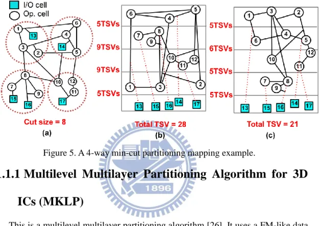
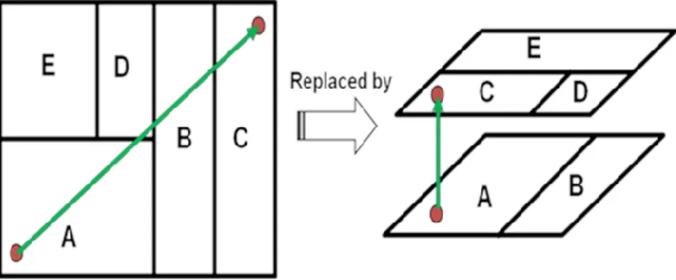
layering, which is a very important issue in 3D partitioning. In Figure 5, an example is

illustrated to show the importance of applying a layer-aware algorithm. The divided

circuit after applying 4-way min-cut partitioning to the original circuit is shown in

Figure 5(a), the total cut size is only 8, but when fitting the divided circuit into a 3D

structure, as shown in Figure 5(b) and Figure 5(c), all the I/O pads must be located at

the bottom-most layer, which indicates that extra TSVs should be added (shown in the

red dotted lines), this is the first thing that layer-unaware algorithms do not consider.

The second thing is that when an initial partitioning result is given, different layer

assignments may end up in different TSV counts, as shown in Figure 5(b) and Figure

5(c), but even the best result shown in Figure 5(c) is worse than the result produced

by iLap [27], which is a layer-aware algorithm. The above information demonstrates

how important it is to use a layer-aware algorithm. Some well-known layer-aware

algorithms are discussed as the following: Jiang proposed an Integer Linear

Programming (ILP) [25] method to find the optimal solution. However, the optimal

result comes with the cost of great runtime. Therefore, the algorithm is only for

small-size problem. MKLP [26] modifies the cost of FM to reflect the true TSV count

5

other existing methods on TSV count. FDPrior [28] proposes a force-directed

approach based on N-Body simulation and achieves massive parallelism by GPGPU.

We will discuss some of the algorithms in detail and give some examples to show

how those algorithms minimize the number of TSVs.

Figure 5. A 4-way min-cut partitioning mapping example.

1.1.1 Multilevel Multilayer Partitioning Algorithm for 3D

ICs (MKLP)

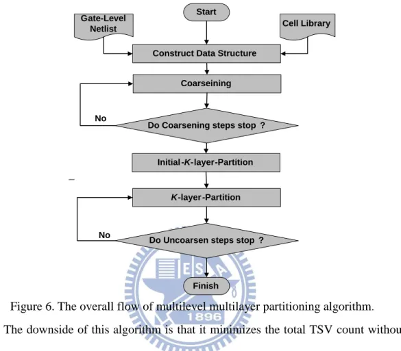
This is a multilevel multilayer partitioning algorithm [26]. It uses a FM-like data

structure but modifies the cost of FM in order to reflect the true TSV count in 3D

structure.

The flow of this algorithm is illustrated in Figure 6. After reading input and

constructing the data structure, coarsening technique is applied to construct a

sequence of successively smaller hypergraph, and then k-layer partition is applied to

the smallest graph to find an initial location for each cell. After finding the initial

partitioning, a k-layer refinement partitioning process is repeatedly applied while

6

refinement phase tends to improve the TSV count. The overall process is terminated

when the original graph is reached.

Figure 6. The overall flow of multilevel multilayer partitioning algorithm. The downside of this algorithm is that it minimizes the total TSV count without

taking the maximum number of TSV count between adjacent layers into account. In

the next section, we will introduce an algorithm which considers both total number of

TSVs and maximum number of TSVs.

1.1.2 Layer-Aware

Design

Partitioning

for

Vertical

Interconnect Minimization (iLap)

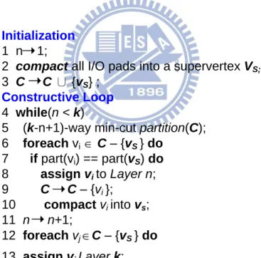
In this section, we introduce an iterative k-way min-cut partitioning algorithm

[27]. It not only produces fairly good result on TSV count, but also prevents the burst

number of TSVs between any adjacent layers.

The pseudo code of iLap is shown in Figure 7. Since all the I/O pads must be located at the bottom-most layer, the first step of iLap is to compact all the I/O pads

Start

Construct Data Structure

Coarseining Gate-Level

Netlist Cell Library

Do Coarsening steps stop ?

Initial -K-layer-Partition

K-layer -Partition

Do Uncoarsen steps stop ?

Finish No

7

into a supervertex vs and keep all the related edges unchanged. Then apply k-way

area-balanced min-cut partitioning to the design to get k partitions, note that the area

of vs is set to zero to avoid interfering area balancing when performing partitioning.

After min-cut partitioning, among these k partitions, only one partition ps contains vs,

this implies that the cells in ps have stronger connection with the I/O pads and

therefore should be located in layer 1. The remaining procedure is similar to what we

just described, compact the cells in layer 1 into vs and then apply k-1 area-balanced

min-cut partitioning to decide a set of cells which should be located in layer 2. Repeat

the process until all the layers are determined. We give an example to show how iLap

works when k = 4 in Figure 8.

Initialization

1 n 1;

2 compact all I/O pads into a supervertex VS;

3 C C ∪ {vS} ;

Constructive Loop

4 while(n < k)

5 (k-n+1)-way min-cut partition(C); 6 foreach vi Î C – {vS } do 7 if part(vi) == part(vS) do 8 assign vi to Layer n; 9 C C – {vi }; 10 compact vi into vs; 11 n n+1; 12 foreach vj ÎC – {vS } do 13 assign vj Layer k;

8

Figure 8. An iLap example when k = 4.

1.1.3 A

Force-Directed

Based

Parallel

Partitioning

Algorithm for Three Dimensional Integrated Circuits

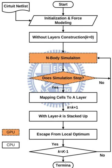
on GPGPU (FDPrior)

A novel force-directed algorithm on GPGPU is proposed in this work [28]. The

method is different from other traditional partitioning algorithms by using a

force-directed way based on N-Body simulation to divide the circuit.

The overall flow of the algorithm is shown in Figure 9. Three phases are

consisted in the algorithm. In phase 1, the motion of each cell is simulated by the

connectivity among each cell and its neighbors. The idea of this phase is adopted from

N-Body simulation. The purpose of phase 2 is to find a set of appropriate cells to

construct the current layer. Since this is a bottom-up approach, cell at lower position

means that it has stronger connection with the bottom cells, hence should be given a

higher priority to be located in the current layer. The cells included in this layer are

9

position in order to escape local optimum in phase 3. Repeat the process until all the

layers are constructed. The major advantage of using N-Body simulation is that when

simulating the system, the motion of each cell is assumed to be independent to each

other. Therefore GPGPU can be applied to achieve massive parallelism. However, the

TSV result produced by FDPrior is worse than iLap’s due to the lack of counting real

TSV count.

Cirtuit Netlist Start

Initialization & Force Modeling

N-Body Simulaiton

Does Simulation Stop?

Mapping Cells To A Layer

With Layer-k is Stacked Up

Escape From Local Optimum

k=K-1

Without Layers Construction(k=0)

Termina Yes No No Yes k=k+1 GPU CPU

Figure 9. The overall flow of FDPrior.

1.2 Introduction to GPGPU

The full name of GPU is graphic processing units, which is obviously designed

for operating graphic computing; and for GPGPU, as the name implies, GPGPU

10

of other applications rather than just graphic. Since it is quite different from the

conventional CPU, a brief introduction about the architecture of GPGPU and its

platform is given in the following section.

1.2.1 Difference between GPU and CPU

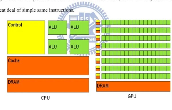
GPU is designed for compute-intensive and massive parallel computing. The

characteristic of GPU is highly parallelism, it has much more processing units but

lower working frequency compared to CPU. And those processing units are

specifically designed for data processing rather than flow control. In Figure 10, we

illustrate the major structure difference between GPU and CPU. CPU is capable of

any kinds of complicated instructions. On the other hand, GPU can only handle a

great deal of simple same instructions.

Figure 10. CPU versus GPU.

1.2.2 Compute Unified Device Architecture (CUDA)

CUDA is a general purpose parallel computing architecture invented by NVIDIA

11

CUDA programs can be implemented in C or C++. The programming model of

CUDA is single instruction multiple threads (SIMT), which means each thread

executes the same instruction but owns different data. NVIDIA further provides a way

to let programmers control these threads.

In CUDA architecture, the basic operating unit is a thread, a block consists of a

group of threads, and a grid is a group of blocks. Each thread has its own register.

Threads in the same block can synchronize with each other and exchange their data

through shared memory. On the other hand, threads in different blocks cannot

synchronize and can only exchange data through global memory.

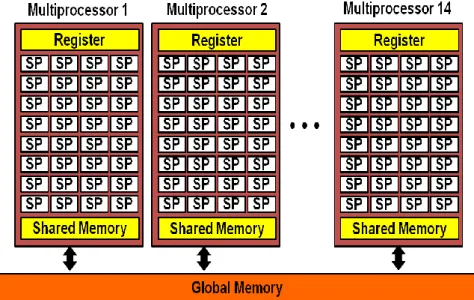
A block corresponds to a multiprocessor (MP). Each MP includes many single

precision float stream processors (SP). SP is the basic processing unit, therefore is in

charge of all the computing and every SP corresponds to a thread. In Figure 11, we

show the hardware architecture of NVIDIA Tesla M2050, each MP consists of 32

SPs, and there are 14 MPs, hence, it is able to process 32 x 14 = 448 single precision

float operations simultaneously at most if we do not switch threads.

12

1.2.3 CUDA Device Memory

Memory structure in GPU is entirely different from CPU. Therefore we give an

overview about some common used device memory of CUDA in Figure 12. The

latency of shared memory is about 100 times faster than global memory, but the

capacity of shared memory is usually small (16k bytes in Tesla architecture), this may

influence the performance.

Memory Type Scope Hardware Latency

Global Grid DRAM 400-600 clock

Local Thread DRAM 400-600 clock

Register Thread On GPU Immediate

Shared Block On GPU 4-6 clock

Figure 12. CUDA memory overview.

1.3 Thesis Organization

Our thesis organization is listed as the following. In chapter 2, we show our

motivations and the problem formulation. In chapter 3, we will demonstrate our

proposed algorithm step by step. In chapter 4, we present our experimental results.

13

Chapter 2

Problem Formulation

In this chapter, we show our motivations and problem formulation.

2.1Motivations

In section 1.2.2, we demonstrated the algorithm flow of iLap, we can conclude

that iLap is quite powerful and outperforms all the other previous works in TSV

count. The drawback of iLap is its runtime. In Figure 13, the blue line (line with

squares) represents the runtime of iLap, it is obvious that the runtime of iLap grows

linearly as the number of layer grows. This is caused by its iterative k-way min-cut

partitioning methods. We have introduced the overall process of iLap in the previous

section, we know that k-way min-cut partitioning is applied first and then (k-1)-way

min-cut partitioning, (k-2)-way min-cut partitioning, etc. Each time after the

partitioning process, 1/k of the circuit is compacted into a supervertex, the compacting

step is able to reduce the problem size. Therefore, the problem size is reduced in an

order of (k-1)/k, (k-2)/k, (k-3)/k, etc, which means for larger k, the reduction ratio of

problem size gets smaller, this is the main reason for the linear growing runtime when

14

Figure 13. The execution time of iLap compared to other algorithms [27].

Since the TSV result of iLap is fairly good, to develop an algorithm similar to the

idea of iLap but works in a faster way is our goal, and we hope to further reduce the

runtime by multi-core. And after the step we just described, an additional step is

added to fine tune the result of iLap, this step is also parallelized by multi-core.

After the process we mentioned above, we want another refinement phase. In

section 1.3, we give a brief introduction to GPGPU, GPGPU is known for its

capability of exploiting parallelism. Given such a powerful platform, finding an

algorithm which can benefit from this robust platform is our goal.

2.2 Problem Descriptions

2.2.1 Definitions

A circuit is modeled as a hypergraph G = (V ,E), the meaning of each notation is

listed as the following:

V : A set of cells that each cell vi Î V. Avi : The area of cell vi.

15

E : A set of hyperedges that connects more than one cell. Every hyperedge is a subset of V, e  V, e Î E.

Alayer_j : Total area of all cells in layer j.

Aavg : The average of the total area in k layers,

Aavg = ( .

r : A given constant that decides the area bound ( 0< r < 1 ). Amin : The minimal allowed area for all layers, Amin= Aavg * (1 – r).

Amax : The maximal allowed area for all layers, Amax= Aavg * (1 + r).

2.2.2 Problem Formulation

In this thesis, we model the 3D IC partitioning problem as a layer-aware

multi-layer 2-way min-cut partitioning problem. Given a k-layer 3D structure, a

design G=(V,E), I/O constraint and area constraint ( ). The

16

Chapter 3

Proposed Algorithm

In this chapter, we show our parallel layer-aware partitioning algorithm step by

step. Two phases are included in our flow. The first phase is a deterministic phase and

the second phase is a stochastic phase.

3.1 Deterministic Phase

In this phase, we propose an iterative 2-way min-cut partitioning method which

is called divergent step. And after that, 2-way min-cut is applied to some of the

partitions in order to achieve better solution quality, this phase is called convergent

phase.

3.1.1 Divergent Step

Our goal in this step is to find a feasible solution as quick as possible. We know

that all the I/O pads must be located at layer 0 in 3D structure. Hence the number of

TSVs between layer 0 and other upper layers are fixed at the beginning. This concept

is shown in Figure 14. Since layer 0 is already decided, we can gradually obtain our

result based on these fixed I/O pads.

A tree structure is used to present the flow of this step. Therefore, we give some

definitions first. Assume we have a tree node n:

n.c : Cells needed to be divided in this partitioning process.

17

different layers compared to n.c, n.rc = V – {n.c}.

n.bl : The possible bottom-most layer for n.c.

n.nl : Number of layers n.c spans over.

The variables we just described are not easy to understand, therefore an example

in Figure 15 is given to show what those variables mean. In Figure 15, the value of

n.bl and n.nl are 2 and 3 respectively, this means that the lowest possible location for n.c starts from layer 2 and spans over 3 layers, which indicates layer 2, layer 3 and

layer 4 are possible layer locations for n.c. The above information further implies that

when n.nl is not equal to 1, n.c needs to be further divided; and when n.nl is equal to

1, n.c is fixed at layer n.bl.

Figure 14. The initial TSV count caused by I/O pads.

18

Before starting, one important concept must be brought in. When performing

min-cut partitioning on n.c, all the cells in n.rc are compacted into two types of

supervertices and their area are set to zero to avoid interfering area balancing. This is

because when performing partitioning on n.c, we are basically deciding layer (n.bl to

n.bl + n.nl -1), hence the area of cells in other layers shouldn’t be taken into consider.

And according to the location of n.rc, there are two types of supervertices: vb and vt.vb means the location of this supervertex is lower than n.c’s; similiarly, vt means the

location of this supervertex is higher than n.c’s. We have showed all the definitions

needed for our flow, in the remaining part of this section, an example when k = 4 is

given to show how our flow goes. To simplify the problem in our example, the area of

each cell is set to 1.

In the beginning, only one node exists in the tree. The initial tree information is

illustrated in Figure 16. Assume we name the root node A. Before the process starts,

all the cells clearly needed to be partitioned, therefore, all the cells but I/O pads are

included in A.c and all the I/O pads are included in A.rc since I/O pads are obviously

located at a lower layer than A.c. All I/O pads are compacted into a supervertex vb as

shown in Figure 17. The lowest possible layer for A.c is 1, hence A.bl = 1. Since we

are dividing the circuit into 4 layers, A.nl = 4.

19

Figure 17. Compact cells into a supervertex vb.

Then enters the next step, we called this step "the first partition", the purpose of

this process is to find a set of cells that should be located near the I/O pads, which

means finding a set of cells that has higher connectivity with the I/O pads. What we

do is perform 2-way area-balanced min-cut partitioning on the design shown in Figure

18. The reason for performing 2-way min-cut partition is that it can produce the result

in an acceptable time and can divide the problem size into half, which might shorten

the runtime in the succeeding procedure. After 2-way partitioning, all the cells are

divided into two groups of cells. Only one group contains the supervertex vb, we call

it pb, cells in pb should be located closer to I/O pads. And since k = 4, pb contains 2

layers of cells from layer 1 to layer 2; and the other group, we call it pt, not containing

vb, needless to say contains cells from layer 3 to layer 4. All the information we just mentioned is illustrated in Figure 18. Now, we map the result into our tree structure.

The root node A has two children nodes B and C. pb becomes B.c, which is the set of

cells needed to be further partitioned in the succeding process. The original

compacted vertex vb already existed in B.rc, and because the cells in pt are now

located in different layers compared to B.c, pt are added to B.rc. The possible

20

The similar idea is applid to tree node C. The tree structure and its information is

shown in the right side of Figure 18.

Figure 18. The first partition of our algorithm and its tree structure.

After the first partition, second partition is now applied to tree node B, before we

do that, we need to compact the cells that located in different layers. The original

compacted cell vb stays unchange, right now we need to compact cells in B.rc except

vb, in Figure 18, we can find that when taking vb away from B.rc, the set of remining cells is equal to the cell set in C.c, which indicates that these cells are located at higer

layers compared to B.c, therefore, we need to compact these cells into a new

supervertex vt. The compacting step is shown in Figure 19. After that, 2-way area

balanced min-cut partitioning is applied again to divide B.c into two groups. We know

that B.nl = 2, which means cells in B.c span over 2 layers. And after 2-way

partitioning, each group of cells corresponds to only 1 layer, this suggests that this

group of cells should be located at this particular layer and thus the layer is fixed.

Since we have divided B.c into two groups, as we said before, the group of cells

containing vb should be located at lower layer, which is layer 1 in this case, and the

21

layer 2 are both fixed after this step. We illustrate the information above in Figure 20

shown in a tree.

Figure 19. The second partition of our algorithm.

Figure 20. The tree structure after the second partition in our algorithm.

The third partition performed on C.c is similar to the second partition, except that

in the third partition, all the cells in C.rc are compacted into vb since their locations

are all definitely lower than C.c. We have showed plenty of details in the first two

partitions, therefore the details of the third partition are not descripted word by word.

22

that all the layers are decided and hence end the whole process.

Figure 21. The third partition of algorithm.

Figure 22. The tree structure after the third partition in our algorithm.

The example we just went through has a total layer of 4, which can easily apply

just 2-way area-balanced min-cut partitioning to finish the total flow. When k is not

an even number, the major difference is that we perform 2-way area-unbalanced

min-cut partitioning. We still want to divide the problem size into half to reduce the

succeding runtime, since it is not possible in this case, we try to let the value of area

ratio between these groups approach 1:1 as much as possible, which is set to

((k-1)/2) : ((k+1)/2) here, and the layer ration these two groups correspond to is the

same as area ratio. We demonstrate the flow using our tree structure when k = 7 in

23

Figure 23. The flow of divergent step when k = 7.

Now, we present you the overall flow of divergent step, before we do that, we

want to emphasize several important concepts again. The first thing is that there are

two types of supervertex in our algorithm, it is important to make sure which kind of

supervertex we are compacting. The second thing is that the area of supervertex is

always set to zero, and when compactiong cells into a supervertex, all the edges must

keep unchange. Figure 24 is the pesudo code of this step. To summarize, at the

beginning, we compact all I/O pads into vb, and then build a root node to represent the

initial condition. Then we transverse the tree in BFS order, assume we are trasversing

node n, if n.nl is not equal to one, two children node is generated, then perform 2-way

min-cut partitioning on n.c to get two groups of cells with area ratio (n.nl-1)/2 :

(n.nl+1)/2, and the condition after partitioning is mapped to the children node of n we

just generated. And if n.nl is equal to 1, all cells included in n.c is fixed at layer n.bl

and no child node is generated. The process is repeated until every leaf node n, n.nl

24

Figure 24. Pseudo code of divergent step.

3.1.2 Convergent Step

The divergent process is sometimes too arbitrary due to the flexibility of vertices

which have been limited in the early partitions. The condition after the first partition when k = 8 is shown in Figure 25, if a cell belongs to the group not containing vb after

first partitioning, this means the cell must be located at layers higher than 4 no matter

what happens after that. But what if the best location for that cell is layer 4? In this

phase, we want to respect the solution obtained from previous step but give some cells

a certain degree of freedom trying to fine tune the solution.

Figure 25. The first partition shown in tree structure when k = 8.

In the following, we list all the necessary details for this step: A B C D E F G

25

i) All tree nodes are unlocked at the beginning. Two unlocked adjacent tree

nodes with different parent nodes are merged together and then perform

partition again. This is shown in Figure 26.

ii) If a tree node is not merged, it is then locked for the remaining procedure.

Figure 26. Tree nodes that can be merged and partitioned.

Repeat the process above until no more tree nodes can be merged. We use Figure

27 as an example to show the overall flow of this step. We can see that at the first

level of convergent step, we follow the rules described above to decide which nodes

should be merged. The tree nodes corresponding to the highest layer and the lowest

layer can't be merged, which is quite reasonable, take the highest layer for example,

these cells are here because they have been divided into the group not containing vb

every time they needed to be partitioned, since the decisions have always been the

same for these cells, it is reasonable not to give them any more freedom. And cells

included in the lowest layer are locked for the same reason. But this does not imply

the lowest and the highest layers are always locked, it indicates that the cells in

26

layers. We need two nodes to perform merge and partitioning, therefore cells located

at edge layers are sometimes forced to be included in the process when k is an odd

number.

Figure 27. An example of convergent step when k = 8.

3.1.3 Parallel Scheme

Our parallel scheme is illustrated in Figure 28, it is evident that the partitioning

process on each level is independent to each other. Therefore, we parallelize this

partitioning process on the same level by multi-core. We can also give a comparison

about the total partition count between sequential version and parallel version. For the

sequential version, k-1 runs and ((k-1)/2 + … + 2 + 1) runs are required for divergent step and convergent step respectively; and as we parallelize the procedure,

log2k runs and (k-1)/2 runs are required for divergent step and convergent step

respectively. This indicates that the time complexity for divergent step can be reduced

27

to O(k). One important message showing here is that we are able to save more time as

k increases.

Figure 28. The parallel scheme of first phase.

3.2 Stochastic Phase

In this phase, we perform simulated annealing algorithm [30] combined with

GPGPU to refine the solution. The purpose of using GPGPU is to explore more

solution space in order to find more possibilities.

3.2.1 Simulated Annealing Process

The overall process flow is shown in Figure 29. We use W threads on GPGPU

and each thread runs L evaluations simultaneously [31], every time after L

evaluations, the best result and the temperature is updated on CPU and later

broadcasted to every thread on GPU. The evaluation and update procedure is repeated

28

Solution from previous phase

Evaluate for better

result

Update result & temperature

Meet the terminal criterion? Stop Yes NO W Run L evaluations Evaluate for better result Evaluate for better result Run on GPU Run on CPU

Figure 29. The flow of stochastic phase.

3.2.2 Cost Function and Parameter

There are two types of possible perturbation in our SA process:

i) Move: Pick a random cell, and move it to another layer.

ii) Swap: Random pick two movable cells and switch their positions.

Before describing our cost function and parameter settings, we define some of

the parameters first:

T0 : Initial temperature.

Ti : Processing temperature.

 : Cooling rate. (<1)

29

Equation 1 shows how the temperature is updated.

(1) Every time when a perturbation is applied, a new cost is obtained, and the new

cost is compared with old cost. And in this thesis, cost means the total TSV count.

(2) If the new cost is better, which implies ∆h < 1, the solution is accepted.

However, if ∆h ≥ 1, a random r is generated:

(3) And the worse solution is accepted when equation 4 holds. This indicates that the

probability of accepting a worse solution is given by equation 5.

(4) (5)

Figure 30 shows the plot of exponential function. We can see from the plot that

when Ti approaches infinity, P approaches 1; and when Ti approaches 0, P approaches

0. This indicates how important it is to find an appropriate Ti. Hence, the next section

30

Figure 30. Plot of exponential function.

3.2.3 Parameter Settings

W is set to 256 to exploit the solution space, and we want a slow cooling down

rate, therefore,  is set to 0.95, also, Max_Iteration is set to 20,000. And for the value of L, we have tried many different values of L, L hardly affects the final result, hence

L is set to 100 to prevent large runtime. Most of the values are determined but T0, here, we give a detail discuss about the value of T0. Typical SA usually starts with a

random generated initial solution, and T0 of those SA processes are usually high. In

Figure 31, we show the result of using different T0. The horizontal axis represents the

total iteration counts, and the vertical axis represents the TSV count after the SA

process normalized to the TSV count obtained from previous phase. It is clear that a

peak appears at the beginning of the SA process at every initial temperature. And the

results are all worse than the original results. This is because our solution from

previous phase is already in a good state, setting T0 too high will result in accepting

too many uphill moves at the start and makes it even harder to reach a better solution.

In Figure 32, we further lower the initial temperature. Even when we set a very low

initial temperature to avoid accepting too many bad moves, which basically means

our SA process only accepts good moves, the improvement is still less than 1%. We

conclude that our solution from previous phase is already good. It is hard to achieve

large improvement even though we exhaustively try almost all of the combinations of

31

Figure 31. SA process with different T0.

Figure 32. SA process with different T0.

0 1 2 3 4 5 6 7 8 9

N

o

rm

a

li

z

e

d

T

S

V

c

o

u

n

t

Iteration Count

aqua

T=1000 T=500 T=100 T=50 0.98 0.985 0.99 0.995 1 1.005 1.01 1.015

N

o

rm

a

liz

e

d

T

S

V

c

o

u

n

t

Iteration count

aqua

T=10 T=1 T=0.1

32 .

Chapter 4

Experiments

4.1 Environment Setup

We evaluate the performance of our method and other three methods over a set of

14 test cases, 10 of them are from the MCNC benchmark set [32], one 128-point FFT

design [33], and three other large cases from Altera [34]. The information of these

benchmarks are reported in Table 1. The area of each cell in these cases can be any

number, therefore, the area of each cell is random generated from 1 to 10. And the

parameter that determines the area bound is set to 0.05 like other works. The

experimental results are the average results of ten runs using different random seeds.

And our experiment is implemented on a C++/Linux platform, with an Intel Xeon

2.4GHz CPU. In our second phase, the GPGPU platform is NVIDIA Tesla M2050.

33

The object for comparison is listed as the following:

i) hMetis: hMetis is applied to perform the min-cut partitioning, and then

each part is mapped to a layer in random order [21].

ii) EX-hMetis: hMetis is applied to perform the min-cut partitioning, and

after trying all possible layer permutations, the permutation with the best

TSV count is chosen.

iii) iLap: An iterative layer-aware min-cut partitioning algorithm [27].

4.2 Experimental Results

4.2.1 Number of TSVs of First Phase

In this section, we show the result obtained from the first phase (deterministic

phase) when k = 4 in Table 2. EX-hMetis always picks the best TSV count out of 4! =

24 different possible layer permutations generated from hMetis and therefore

EX-hMetis attains 15% TSV reduction on average compared to hMetis. However, our

method can reduce TSV count by 27% on average as compared to EX-hMetis.

Design # of Nodes# of Nets # of Ios

Tseng 1047 1098 174 Diffeq 1497 1560 103 Des 1591 1847 501 Bigkey 1707 1935 426 Frisc 3556 3575 136 elliptic 3604 3734 245 pdc 4575 4591 56 fft128 4736 5246 766 s38417 6406 6434 135 s38584.l 6447 6484 342 clma 8383 8444 144 cfft 15425 15476 644 aqua 29744 30208 3793 video 53491 55393 5431

34

Moreover, for the largest three test cases (cfft, aqua, and video), our method can even

reduce the TSV count by more than 78% compared to hMetis. And we know that iLap outperforms all other previous works, this indicates that iLap produces fairly good

result, but we can still get a 3% improvement compared to iLap.

Table 2. TSV result comparison of first phase when k = 4.

4Layers Total TSVs Normalized to hMetis Ours Normalized

to iLap Design

Ours iLap hMetis

EX-

hMetis Ours iLap

EX- hMetis Tseng 290 307 363 345 0.80 0.85 0.95 0.95 Diffeq 234 242 321 280 0.73 0.75 0.87 0.97 Des 446 445 851 824 0.52 0.52 0.97 1.00 Bigkey 616 612 666 652 0.93 0.92 0.98 1.01 Frisc 616 657 713 687 0.86 0.92 0.96 0.94 elliptic 565 589 681 640 0.83 0.87 0.94 0.96 pdc _{908 1006 1088 1027 0.83 0.92 0.94 0.90} fft128 1283 1306 1504 1487 0.85 0.87 0.99 0.98 s38417 231 245 351 320 0.86 0.70 0.91 0.95 s38584.l 290 392 683 554 0.57 0.57 0.81 1.00 clma 483 487 714 487 0.68 0.68 0.68 0.99 cfft 228 239 1015 309 0.22 0.24 0.30 0.95 aqua 827 895 6893 5085 0.12 0.13 0.74 0.92 video 757 737 8719 7129 0.09 0.08 0.82 1.03 Average 0.62 0.64 0.85 0.97

In Table 3, we increase the layer from 4 to 8. We can see that the improvement

increases to 39% compared to hMetis, and the improvement compared to iLap even

reach 6%, which is a good sign that our algorithm remains the quality even when

35

Table 3. TSV result comparison of first phase when k = 8.

8Layers Total TSVs Normalized to hMetis Ours Normalized

to iLap Design

Ours iLap hMetis

EX-

hMetis Ours iLap

EX- hMetis Tseng 677 740 860 789 0.79 0.86 0.92 0.91 Diffeq 538 597 760 654 0.71 0.79 0.86 0.90 Des 1075 1087 1977 1880 0.54 0.55 0.95 0.99 Bigkey 1437 1451 1557 1516 0.92 0.93 0.97 0.99 Frisc 1333 1428 1655 1550 0.81 0.86 0.94 0.93 elliptic 1205 1321 1587 1416 0.76 0.83 0.89 0.91 pdc 1918 2171 2447 2199 0.78 0.89 0.90 0.88 fft128 2964 3070 3530 3484 0.84 0.87 0.99 0.97 s38417 530 573 837 749 0.63 0.68 0.89 0.93 s38584.l 936 1022 1669 1367 0.56 0.61 0.82 0.92 clma 1289 1383 1821 1375 0.71 0.76 0.76 0.93 cfft 541 542 2474 704 0.22 0.22 0.28 1.00 aqua 1828 1978 15864 10795 0.12 0.12 0.68 0.92 video 1915 2005 20340 15811 0.09 0.10 0.78 0.96 Average 0.61 0.65 0.83 0.94

4.2.2 Result of Runtimes of First Phase

The runtime comparison is reported in Table 4. The runtime of hMetis and

Ex-hMetis are both quite short. Our algorithm requires longer runtime than hMetis and Ex-hMetis, but given the 38% improvement on TSV count, this is totally acceptable.

And we have a 3% improvement on TSV count compared to iLap, but our runtime is

36

Table 4. Runtime result comparison of first phase when k = 4.

4Layers Execution time (s) Normalized to hMetis Ours Normalized

to iLap Design

Ours iLap hMetis

EX-

hMetis Ours iLap

EX- hMetis Tseng 0.24 0.41 0.20 0.20 1.23 2.11 1.01 0.58 Diffeq 0.34 0.53 0.23 0.23 1.44 2.26 1.00 0.63 Des 0.41 0.70 0.39 0.40 1.04 1.78 1.02 0.58 Bigkey 0.17 0.33 0.15 0.15 1.10 2.17 1.02 0.51 Frisc 0.72 0.94 0.46 0.47 1.57 2.05 1.03 0.77 elliptic 0.56 0.79 0.35 0.36 1.63 2.30 1.05 0.71 pdc 1.10 1.50 0.68 0.70 1.61 2.19 1.02 0.73 fft128 0.54 0.78 0.43 0.45 1.23 1.79 1.04 0.69 s38417 1.03 1.55 0.81 0.83 1.28 1.92 1.02 0.67 s38584.l 1.21 1.90 0.89 0.91 1.36 2.13 1.02 0.64 clma 1.69 2.45 1.26 1.28 1.34 1.94 1.02 0.69 cfft 1.53 2.17 1.15 1.18 1.34 1.89 1.03 0.71 aqua 5.23 6.69 2.76 2.87 1.90 2.43 1.04 0.78 video 8.15 10.7 2 4.34 4.59 1.88 2.47 1.06 0.76 Average 1.42 2.10 1.03 0.67

In Table 5, we increase the layer from 4 to 8. The improvement compared to

iLap increases from 33% to 68%. It is evident that hMetis is very time-efficient. Since EX-hMetis has to go through all possible layer permutations to find the best one, the

required runtime is therefore exponential to the number of layers. The runtime

required by iLap grows linearly due to the multi-way partitioning inside iLap.

Hence, we can conclude that our method can benefit from modern parallel computing

37

Table 5. Runtime result comparison of first phase when k = 8.

8Layers Execution time(s) Normalized to hMetis Ours Normalized

to iLap Design

Ours iLap hMetis

EX-

hMetis Ours iLap

EX- hMetis Tseng 0.41 1.44 0.30 4.15 1.37 4.79 13.82 0.29 Diffeq 0.53 1.64 0.38 5.92 1.38 4.27 15.41 0.32 Des 0.64 2.06 0.60 7.47 1.08 3.47 12.56 0.31 Bigkey 0.32 1.22 0.26 7.07 1.24 4.67 27.09 0.27 Frisc 0.94 2.53 0.66 14.40 1.42 3.83 21.85 0.37 ellipric 0.74 3.81 0.53 14.42 1.38 7.13 27.01 0.19 pdc 1.50 4.04 0.93 21.36 1.61 4.33 22.92 0.37 fft128 0.73 2.35 0.66 15.46 1.10 3.53 23.28 0.31 s38417 1.38 4.55 1.25 25.98 1.10 3.63 20.75 0.30 s38584.l 1.59 5.63 1.37 28.13 1.15 4.10 20.47 0.28 clma 2.32 7.83 1.97 37.27 1.18 3.97 18.91 0.30 cfft 2.00 6.15 1.67 54.04 1.20 3.68 32.38 0.32 aqua 6.40 16.8 6 3.91 204.54 1.64 4.31 52.32 0.38 video 10.7 0 27.3 4 6.18 441.15 1.73 4.43 71.42 0.39 Average 1.33 4.30 27.16 0.32

4.2.3 Speedup Result of First Phase and Discussion

Since multi-core platform is applied for the first phase of our algorithm. In this

section, we show and analysis our speedup result.

First, we define some variables. Since we used a tree structure to represent our

process in first phase, the level of a partition can be calculated using the same way as

a typical tree as shown in Figure 33. time(i) represents the total sequential time of

level i, and core(i) represents the number of cores used in level i. The maximum

38

Maximum speedup =

(6)

Figure 33. Procedure of deterministic phase.

In Table 6, we show the result of our speedup. The speedup is obtained using

equation 7. And the efficiency is calculated as equation 8.

(7)

(8) The result shows that our average efficiency is up to 88%, which is quite efficient,

when increasing layer from 4 to 8, max speedup increases since we are able to use more

cores when the layer increases, but the downside of using more cores is that the

efficiency may drop, we can see from Table 7 that the average efficiency drops to 70%

when k = 8. This is quite reasonable since more time is needed to synchronize when

more cores are used.

39

4Layers _{Speedup Evaluation}

Design Parallel(s) Sequential(s) Speedup Max Speedup Efficiency

Tseng 0.24 0.30 1.24 1.27 0.90 Diffeq 0.34 0.42 1.24 1.30 0.80 Des 0.41 0.47 1.16 1.26 0.61 Bigkey 0.17 0.20 1.21 1.31 0.69 Frisc 0.72 0.87 1.21 1.27 0.76 elliptic ic 0.56 0.72 1.27 1.28 0.98 pdc 1.10 1.37 1.25 1.25 0.98 fft128 0.54 0.66 1.23 1.28 0.81 s38417 1.03 1.29 1.25 1.25 0.99 s38584.l 1.21 1.50 1.23 1.24 0.98 clma 1.69 2.10 1.24 1.25 0.97 cfft 1.53 1.89 1.23 1.24 0.96 aqua 5.23 6.25 1.20 1.21 0.93 video 8.15 9.87 1.21 1.22 0.96 Average 0.88

40

8Layers _{Speedup Evaluation}

Design Parallel(s) Sequential(s) Speedup Max Speedup Efficiency

Tseng 0.41 0.70 1.69 2.10 0.63 Diffeq 0.53 0.91 1.72 2.13 0.64 Des 0.64 1.02 1.58 2.07 0.54 Bigkey 0.32 0.61 1.88 2.22 0.72 Frisc 0.94 1.62 1.73 2.04 0.70 elliptic 0.74 1.33 1.80 2.11 0.72 pdc 1.50 2.73 1.82 2.07 0.76 fft128 0.73 1.29 1.77 2.03 0.75 s38417 1.38 2.52 1.82 2.07 0.76 s38584.l 1.59 2.75 1.74 2.02 0.72 clma 2.32 4.29 1.85 2.00 0.85 cfft 2.00 3.54 1.77 2.08 0.72 aqua 6.40 10.65 1.66 2.01 0.66 video 10.70 17.40 1.63 1.97 0.65 Average 0.70

4.2.4 Speedup Result of Second Phase and Discussion

We mentioned the TSV result of using a massively parallel SA, which is less

than 1% improvement even we exploit the solution space by GPGPU. Here in this

section, we show the speedup achieved by GPGPU compared to the traditional CPU.

We first summarize our parameter settings again: T0 = 1,  = 0.95, W = 256, L = 100 and Max_Iteration is set to 50,000 in order to observe the runtime difference between

CPU and GPGPU more easily. The speedup result is shown in Table 8. We discover

that the average speedup is only 2.18 even we used 256 threads. Why? The first

reason is that GPU is bad at handling branch instructions, which is an instruction

appears a lot in the SA process. And the second reason is the different memory

41

in section 1.3.3, the latency of shared memory is small but the capacity of shared

memory is only 16k bytes; on the contrary, the latency of global memory is large but

the capacity is quite enough. However, the size of our data can only fit into global

memory. The latency of global memory is about 347.83ns ~ 521.74ns, and the

memory latency of CPU is about 1ns to 30ns. We can find that the latency of CUDA

is at least 10 times slower than CPU, which makes a significant impact on the

speedup.

Table 8. Speedup result of second phase when k = 4.

4 Layers Execution Time

Design CPU CUDA Speedup Tseng 3661.91 1980.44 1.85 Diffeq 3759.04 1885.47 1.99 Des 2622.42 1198.73 2.19 Bigkey 4918.97 2614.12 1.88 Frisc 4973.14 2830.73 1.76 elliptic 8255.98 4711.01 1.75 pdc 3545.87 2045.93 1.73 fft128 966.94 295.04 3.28 s38417 5038.52 2843.40 1.77 s38584 13635.55 8063.34 1.69 clma 7603.22 4761.64 1.60 cfft 1599.19 440.98 3.63 aqua 2305.66 750.85 3.07 video 4373.72 1823.03 2.40 Average 2.18

42

Chapter 5

Conclusion

In this thesis, we propose a parallel layer-aware partitioning algorithm for TSV

minimization in 3D ICs, and two phases are included in our algorithm. The first phase

of our algorithm consists of two steps and both steps are deterministic. We apply

2-way min-cut partitioning in this phase and make use of the multi-core platform in

order to further reduce runtime. The second phase is a stochastic process. We

combine SA process with the many-core platform – GPGPU, to exploit the solution

space. The result of second phase indicates that it is difficult to achieve large

improvement by SA when the initial solution is already in a fairly good state. The

experimental results demonstrate that our method can reduce the total TSV count by

about 39% compared to hMetis. It also achieves a 6% improvement compared to iLap,

with 3X runtime improvement. Consequently, due to the parallel nature of our method,

we believe it is capable of generating better TSV-minimized results in an acceptable

43

References

[1] S. Das, A. Fan, K-N Chen, C. S. Tan, N. Checka, and R. Reif, “Technology, performance, and computer-aided design of three-dimensional integrated circuits,” in Proc. Int’l. Symp. on Physical Design, pp. 108-115, 2004.

[2] International Technology Roadmap for Semiconductor. Semiconductor Industry Association, 2005 – 2010.

[3] G. Metze, M. Khbels, N. Goldsman, and B. Jacob, “Heterogeneous integration,” Tech Trend Notes, vol. 12, no. 2, pp. 3, 2003.

[4] K. Banerjee, S. J. Souri, P. Kapur, and K. C. Saraswat, “3-D ICs: a novel chip design for improving deep submicron interconnect performance and systems-on-chip integration,” Proc. IEEE, vol. 89, no. 5, pp. 602–633, May 2001.

[5] Y. Xie, G. H. Loh, B. Black, and K. Bernstein, “Design space exploration for 3D architectures,” J. Emerg. Technol. Comput. Syst., vol. 2, no. 2, pp. 65–103, 2006.

[6] R. R. Tummala and V. K. Madisetti, “System on chip or system on package?” IEEE Design & Test of Computers, vol. 16, no. 2, pp. 48 – 56, Apr. – Jun., 1999. [7] C. Ferri, S. Reda, and R. I. Bahar, “Parametric yield management for 3D ICs: models and strategies for improvement,” J. Emerg. Technol. Comput. Syst., vol. 4, no. 4, Article ID 19, Oct. 2008.

[8] G. H. Loh, Y. Xie, and B. Black, “Processor design in 3D die-stacking technologies,” IEEE Micro, vol. 27, pp. 31–48, May-June 2007.

[9] X. Dong and Y. Xie, “System-level cost analysis and design exploration for three-dimensional integrated circuits,” in Proc. ASP-DAC, pp. 234-241, 2009. [10] SOCcentral. [Online]. Available: http://www.soccentral.com.

[11] I. Kaya, S. Salewski, M. Olbrich, and E. Barke, “Wirelength reduction using 3D physical design,” Int’l Workshop Integrated Circuit System Design, pp. 453–462, 2004.

[12] A. Rahman and R. Reif “System-level performance evaluation of three-dimensional integrated circuits,” IEEE Trans. Very Large Scale Integration Systems, vol.8, no.6, pp. 671–678, Dec. 2000.

[13] Kaya, S. Salewski, M. Olbrich, and E. Barke, “Wirelength reduction using 3D physical design,” Int’l Workshop Integrated Circuit System Design, pp. 453–462, 2004.

44

[14] I. Loi, S. Mitra, T. H. Lee, S. Fujita, and L. Benini, “A low-overhead fault tolerance scheme for TSV-based 3D network on chip links,” Proc. Int’l Conf. Computer-Aided Design, pp. 598–602, 2008.

[15] W. R. Davis, J. Wilson, S. Mick, J. Xu, H. Hua, C. Mineo, A.M. Sule, M. Steer, and P. D. Franzon, “Demystifying 3D ICs: the pros and cons of going vertical,” IEEE Design & Test of Computers, vol. 22, no. 6, pp. 498–510, Nov.–Dec. 2005. [16] D. H. Kim, K. Athikulwongse, and S. K. Lim, “A study of through-silicon-via impact on the 3D stacked IC layout,” Proc. International Conference on Computer-Aided Design, pp. 674 – 680, 2009.

[17] E. Beyne et al. “Through-silicon via and die stacking technologies for microsystems-integration,” Proc. IEEE International Electron Devices Meeting, pp. 1 – 4, Dec. 2008.

[18] D. H. Kim, S. Mukhopadhyay, and S. K. Lim. “Through-silicon-via aware interconnect prediction and optimization for 3D stacked ICs,” SLIP, pp. 85–92. 2009.

[19] T. Yan, Q. Dong, Y. Takashima, and Y. Kajotani, “How does partitioning matter for 3D Floorplanning?” Proc. GLSVLSI, pp. 73-78, 2006.

[20] C. M. Fiduccia and R. M. Mattheyses, “A linear time heuristic for improving network partitions,” Proc. Design Automation Conference, pp.175 – 181, 1982. [21] G. Karypis, R. Aggarwal, V. Kumar, and S. Shekhar, “Multilevel hypergraph

partitioning: applications in VLSI domain,” Transactions on VLSI Systems, vol. 7, no. 1, pp. 69 – 79, Mar. 1999

[22] K. Siozios, A. Bartzas, and D. Soudirs, “Architecture-level exploration of alternative interconnection schemes targeting to 3D FPGAs: a software-supported methodology,” International Journal of Reconfigurable Computing, vol. 2008, Article ID 764942, 2008.

[23] C. Ababei and K. Bazargan, “Non-contiguous linear placement for reconfigurable fabrics,” Proc. Reconfigurable Architectures Workshop, pp. 141 – 148, 2004.

[24] C. Ababei, H. Mogal, and K. Bazargan, “Three-dimensional place and route for FPGAs,” Transactions on Computer-Aided Design of Integrated Circuits and Systems, vol. 25, no. 6, pp. 1132 – 1140, Jun. 2006.

[25] I. H.-R. Jiang, “Generic integer linear programming formulation for 3D IC partitioning,” 22nd IEEE International SOC Conference, pp. 321 – 324, 2009.

45

[26] Y. L. Chung, Y. C. Hu, and M. C. Chi, “A multilevel multilayer partitioning algorithm for three dimensional integrated circuits,” International Symposium on Quality Electronic Design, pp. 483 – 487, 2010.

[27] Y.-S. Huang, Y.-H. Liu, and J.-D. Huang, “Layer-aware design partitioning for vertical interconnect minimization”, IEEE Computer Society Annual Symposium on VLSI, pp. 144 – 149, 2011.

[28] W. J. Chen, H.K. Kuo, T. H. Chiu, and B. C. C. Lai, “FDPrior: a force-drected based parallel partitioning algorithm for three dimensional integrated crcuits on GPGPU,” IEEE International Symposium on VLSI Design, VLSI-DAT, pp. 1 – 4 , Apr. 2011.

[29] http://www.nvidia.com.tw/page/home.html

[30] D. Kolar, J. D. PukSec and I. Branica, “VLSI Circuit Partition Using Simulated Annealing Algorithm”, Electrotechnical Conference, vol. 1, pp. 205 – 208, May 2004.

[31] Y. Han, S. Roy, and K. Chakraborty, “Optimizing aimulated annealing on GPU: a case study with IC floorplanning,” International Symposium on Quality Electronic Design, pp. 1 – 7, 2011.

[32] S. Yang, “Logic synthesis and optimization benchmarks user guide,” Technical Report 1991-IWLS-UG-Saeyang, Microelectronics Center of North Carolina, 1991.

[33] T. H. Cormen, C. E. Leiserson, R. L. Rivest, and C. Stein, Introduction to Algorithms, 2nd ed. MIT Press and McGraw-Hill Higher Education, 2001

[34] http://www.eecs.berkeley.edu/~alanmi/benchmarks/altera/old/altera12_blif_baf. zip.