以類神經網路為基礎的通訊等化器之研究

全文

(1)國立交通大學電子工程學系電子研究所. 博士論文. 以類神經網路為基礎的通訊等化器之研究 The Study of Neural-based Channel Equalizers. 研究生：許騰仁指導教授：李鎮宜. 中華民國九十五年七月.

(2) 以類神經網路為基礎的通訊等化器之研究 The Study of Neural-based Channel Equalizers 研究生：許騰仁指導教授：李鎮宜. Student： Terng-Ren Hsu 博士. Advisor： Dr. Chen-Yi Lee. 國立交通大學電子工程學系電子研究所博士論文. A Dissertation Submitted to Department of Electronics Engineering & Institute Electronics College of Electrical and Computer Engineering National Chiao Tung University in Partial Fulfillment of the Requirements for the Degree of Doctor of Philosophy in Electronics Engineering July 2006 Hsinchu, Taiwan, Republic of China.. 中華民國九十五年七月.

(3) 以類神經網路為基礎的通訊等化器之研究研究生：許騰仁指導教授：李鎮宜教授國立交通大學電子工程系電子研究所. 摘要在實際的通訊系統中需要以資料等化器來回復一個失真信號的原始波形，近來許多以類神經網路為基礎的等化器設計被應用在嚴重失真的信號回復。在本文，我們提出了一個新的類神經網路模式，使用一個多變數冪級數函數做為人工神經元的集成函數，應用於多層認知器結構倒傳遞類神經網路，由於對應的訓練演算法是以最陡坡降法推導，故收斂解存在。與使用一階多變數多項式當集成函數的傳統方法相比較，這個新方法的樣本空間分割邊界，將由傳統的片段線性分割變成片段非線性分割，傳統的多層認知器結構倒傳遞類神經網路可視為這個新方法的一個線性特別解。因此，可說這個新的模式是一般化的多層認知器結構倒傳遞類神經網路，與其他的片段線性分割的方法相比較，這個新方法因為具有片段非線性分割樣本空間的能力，所以在應用上有更大的彈性。在有線通訊系統中，我們將以多層認知器結構倒傳遞類神經網路為基礎的通道等化方法應用於不同的地方，在資料速率大於通道頻寬十倍左右的有線頻寬受限通道上，與傳統上使用最小均方誤差演算法為基礎的決策回授等化器相比較，以多層認知器結構倒傳遞類神經網路為基礎的決策回授等化器可提供比較好的效能、容忍比較多的取樣時脈歪斜和允許比較大的通道嚮應變異。然而對於具有非線性失真的嚴重碼際干擾通道來說，以多層認知器結構倒傳遞類神經網路為基礎的決策回授等化器還有改善的空間，使用一般化的多層認知器結構倒傳遞類神經網路為基礎的決策回授等化器可以提供更好的效能。在多條平行的有線頻寬受限通道上，我們採用多輸入多輸出的以多層認知器結構倒傳遞類神經網路為基礎的決策回授等化器和多輸入多輸出的以一般化多層認知器結構倒傳遞類神經網路為基礎的決策回授等化器，同時抑制碼際干擾、串音干擾和背景雜訊。同樣的，多輸入多輸出的以一般化多層認知器結構倒傳遞類神經網路為基礎的決策回授等化器優於多輸入多輸出的以多層認知器結構倒傳遞類神經網路為基礎的決策回授等化器，而且多輸入多輸出的. -i-.

(4) 以多層認知器結構倒傳遞類神經網路為基礎的決策回授等化器又優於使用最小均方誤差演算法為基礎的決策回授等化器。對於無線通訊系統，我們提出一個以多層認知器結構倒傳遞類神經網路為基礎的改進方法。在多路徑平坦衰減通道中，我們應用軟性輸出和軟性決策回授的結構於一個以多層認知器結構倒傳遞類神經網路為基礎的通道等化器，並於其後串接一個軟性決策通道解碼器以改進整體的效能。此外，利用輸出層神經元的轉移函數尺度因子的最佳化，以及在訓練型樣加入少量的隨機擾動，可以進一步的改善以多層認知器結構倒傳遞類神經網路為基礎的軟性決策回授等化器的效能。由模擬結果，在多路徑平坦衰減通道中，使用包含位元交錯的軟性決策通道解碼器時，以多層認知器結構倒傳遞類神經網路為基礎的軟性決策回授等化器的效能優於以多層認知器結構倒傳遞類神經網路為基礎的決策回授等化器和軟性輸出的以多層認知器結構倒傳遞類神經網路為基礎的決策回授等化器。. -ii-.

(5) The Study of Neural-based Channel Equalizers Student: Terng-Ren Hsu Advisor: Chen-Yi Lee Department of Electronics Engineering, National Chiao-Tung University. Abstract In practical communication systems, it is necessary to apply data equalizers to recover the original waveform from the distorted one. Recently, various equalizer designs based on artificial neural networks have been studied to the severely distorting signal recoveries. In this study, we propose a new neural network model that applies a multivariate power series as the summation function of the MLP/BP neural networks. The corresponding training algorithm is deduced by the gradient steepest descent method; consequently, the convergence solutions exist. Compared to the conventional approach using a first order multivariate polynomial, the boundaries separating the pattern space change from piecewise linear into piecewise nonlinear. The traditional method is a special case of the proposed model. Therefore, this new model is a generalized MLP/BP neural network that is more flexible than other piecewise linear approaches because of the nonlinear separating pattern space. For wireline communications, we apply the MLP/BP-based channel equalization schemes to different applications. In wireline band-limited channels that the data rate is about ten times as much as the channel bandwidth, the MLP/BP-based DFEs provide better performance, tolerate more sampling clock skew, and permit larger channel response variance than LMS DFEs. However, the BER performance of the traditional MLP/BP-based DFEs is not good enough for the severe ISI channels with nonlinear distortions. In such channels, the generalized MLP/BP-based DFEs can outperform the -iii-.

(6) traditional MLP/BP-based DFEs that do better than the LMS DFEs. In wireline band-limited parallel channels, the MIMO MLP/BP-based DFEs and the MIMO GMLP/BP-based DFEs can suppress ISI, CCI and AWGN, simultaneously. By the simulation results, the MIMO GMLP/BP-based DFE can yield a substantial improvement over the MIMO MLP/BP-based DFE that perform better than the LMS DFEs in such channels. For wireless communications, a modified approach, which is also based on the MLP/BP neural network, is presented. We apply the soft output and the soft decision feedback structure to the MLP/BP-based channel equalization scheme that concatenates with the soft decision channel decoder to improve whole performance on multi-path fading channels. Moreover, the performance of the MLP/BP-based soft DFE is also increased with the optimal scaling factor searching of the transfer function in the output layer of the MLP/BP neural networks and extra small random disturbances added to the training data. By the simulations, the MLP/BP-based soft DFEs with bit-interleaved TCM outperform the MLP/BP-based DFEs with bit-interleaved TCM and the soft output MLP/BP-based DFEs with bit-interleaved TCM in multi-path fading channels.. -iv-.

(7) Acknowledgements 在這九年的博士班求學過程中，非常感謝指導教授李鎮宜老師的教導，他給學生寬廣的研究自由度，讓創意可以不受限制的盡情發展，並提供良好的研究環境，讓靈感得以驗證實現。在我研究類神經網路的過程中，基礎觀念的建立必須感謝我就讀逢甲大學自動控制工程研究所碩士班時的指導教授蕭肇殷博士和賴啟智副教授，也要謝謝逢甲大學資電學院院長邱創乾教授的教導和關心。此外，感謝口試委員的指導與寶貴的意見。在我的博士論文研究過程中，特別的感謝給許騰尹和林建青，因為你們的大力幫忙，我的研究才能順利完成。也感謝 University of Minnesota 的 Dr. Yi-ru Chen 和 Prof. Simo Sarkanen 在百忙中抽空幫我修改投稿期刊論文的英文稿件。另外感謝 SI2 實驗室的大師兄蔡哲民學長、有革命情感的張錫嘉、李有山、謝百舉、蘇浩坤、羅偉仁、陳麒旭、楊鎮澤、彭文孝、鍾菁哲、王中正、劉益全、蔡尚峰、劉軒宇、曾順得、陳黎峰、蔡侑庭、游瑞元、陳志龍、賴名威、郭子菁、周伶霞、SI2 實驗室的其他同仁、資工 ISIP 實驗室的林祐賢和其他的學弟、明新科大電子系陳啟文主任、鄧俊修學長、呂明峰學長、李纪萍學長、鴻友科技同事樊勁志先生，謝謝你們的關心和協助。最後，謹以此論文獻給我敬愛的母親，也以此紀念我的父親，感謝父母的照顧和栽培。此外姊姊的關心和學習路上一路相伴的弟弟，謝謝你們給我最大的支持與鼓勵，也謝謝內人怡霈的陪伴和照顧小孩的辛苦。. -v-.

(8) 人生無常，不是每件事都會有好的結果。在我最鬱悶的時候帶來最大的欣喜，卻在一切將要順利之際，給我嘎然而止的震驚。淺淺的緣分，一生的思念。. -vi-.

(9) Contents. Abstract in Chinese. i. Abstract. iii. Acknowledgements. v. Contents. vii. List of Tables. xi. List of Figures. xiii. 1. Introduction. 1. 1-1 Thesis Motivation. 1. 1-2 Paper Survey. 4. 1-3 Thesis Organization. 9. 2. Generalized MLP/BP Neural Networks 2-1 Traditional MLP/BP Neural Networks. 11 12. 2-1-1 Architecture. 12. 2-1-2 Backpropagation Algorithm. 14. 2-2 Generalized MLP/BP Neural Networks. 18. 2-1-1 Architecture. 19. 2-1-2 Corresponding Backpropagation Algorithm. 20. 2-3 Complexity Analysis. 24. -vii-.

(10) 3. SISO GMLP/BP-based DFEs for Wireline Applications. 27. 3-1 MLP/BP-based DFEs with High Skew Tolerance for Band-limited Channels. 28. 3-1-1 System Overview. 28. 3-1-2 MLP/BP-based DFEs. 32. 3-1-3 Simulation Results. 33. 3-1-4 Summary. 43. 3-2 GMLP/BP-based DFEs for Severe ISI Channels with Nonlinearity. 44. 3-2-1 Severe ISI Channels and Nonlinear Distortions. 45. 3-2-2 GMLP/BP-based DFEs. 49. 3-2-3 Simulation Results. 51. 3-2-4 Summary. 62. 4. MIMO GMLP/BP-based DFEs for Wireline Applications 4-1 MIMO MLP/BP-based DFEs for Overcoming ISI and CCI. 63 64. 4-1-1 Multi-channel Environment. 64. 4-1-2 MIMO MLP/BP-based DFE. 68. 4-1-3 Simulation Results. 69. 4-1-4 Summary. 79. 4-2 MIMO GMLP/BP-based DFEs for Overcoming ISI and CCI. 80. 4-2-1 Multi-channel Environment within a Plane. 81. 4-2-2 MIMO GMLP/BP-based DFE. 82. 4-2-3 Simulation Results. 83. 4-2-4 Summary. 87. -viii-.

(11) 5. MLP/BP-based Soft DFEs with TCM for Wireless Communications. 89. 5-1 Wireless Channel Environment. 90. 5-2 Error Control Coding. 93. 5-3 Architecture. 93. 5-3-1 The MLP/BP-based Soft DFEs. 94. 5-3-2 Soft Decision Channel Coding and Interleaving. 96. 5-4 Simulation Results. 96. 5-5 Summary. 103. 6. Conclusion and Future Works. 105. 6-1 Conclusion. 105. 6-2 Future Works. 107. References. 109. -ix-.

(12) -x-.

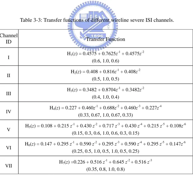
(13) List of Tables Table 2-1: The comparison of computational complexity.. 25. Table 3-1: Transfer functions of several wireline band-limited channels.. 31. Table 3-2: The comparison of sampling clock skew tolerance.. 44. Table 3-3: Transfer functions of different wireline severe ISI channels.. 47. Table 3-4: The BER vs. SNR performance comparison with different equalizers for Channel 1, 2, and 3 without truncations at BER = 10-4.. 61. Table 3-5: The BER vs. SNR performance comparison with different equalizers for Channel 1, 2, and 3 with 30% truncations at BER = 10-3.. 62. Table 4-1: Weighting of co-channel interference between different channels in space.. 67. Table 4-2: Simulation conditions for MIMO MLP/BP-based DFE.. 71. Table 4-3: Weighting of co-channel interference between different channels 81. on a plane.. Table 4-4: Simulation conditions for MIMO GMLP/BP-based DFE.. 86. Table 5-1: System configurations and simulation conditions.. 99. Table 5-2: The PER and BER performance improvement.. 103. -xi-.

(14) -xii-.

(15) List of Figures Fig. 2-1: MLP Neural Network Architecture.. 13. Fig. 2-2: Neuron of MLP Neural Networks.. 14. Fig. 2-3: Neuron of Generalized MLP/BP Neural Networks.. 19. Fig. 3-1: System diagram.. 30. Fig. 3-2: Equivalent model for the band-limited channels.. 30. Fig. 3-3: Frequency responses of several similar wireline band-limited channels.. 31. Fig. 3-4: MLP/BP-based DFEs.. 32. Fig. 3-5: BER performance for different types of equalizers in different channels.. 35. Fig. 3-6: BER performance for different types of equalizers with different clock skews in Channel 1.. 36. Fig. 3-7: BER performance for different types of equalizers with different 36. clock skews in Channel 3.. Fig. 3-8: BER performance for different types of equalizers with different clock skews in Channel 5.. 37. Fig. 3-9: BER performance for different channel conditions with regular input pattern configuration at SNR=20dB.. -xiii-. 37.

(16) Fig. 3-10: BER performance for different channel conditions with modified input pattern configuration at SNR=20dB.. 38. Fig. 3-11: BER performance for different ADC resolution at SNR=15, 40. SNR=18, and SNR=20.. Fig. 3-12: BER performance with different ADC resolution.. 40. Fig. 3-13: BER performance for different ADC resolution with internal resolution enhancement.. 41. Fig. 3-14: BER performance for different types of equalizers in different channels.. 41. Fig. 3-15: BER performance for different types of equalizers with different clock skews in Channel 3.. 42. Fig. 3-16: BER performance for different channel conditions with modified input pattern configuration at SNR=20dB.. 42. Fig. 3-17: Equivalent model for the severe ISI channels.. 47. Fig. 3-18: Frequency responses of different severe ISI channels.. 48. Fig. 3-19: The comparison of the transmitted data and the received waveform.. 48. Fig. 3-20: Generalized MLP/BP-based DFEs.. 50. Fig. 3-21: Minimum MSE and standard deviation of MSEs of the training set in Channel 1 at SNR=15dB.. -xiv-. 56.

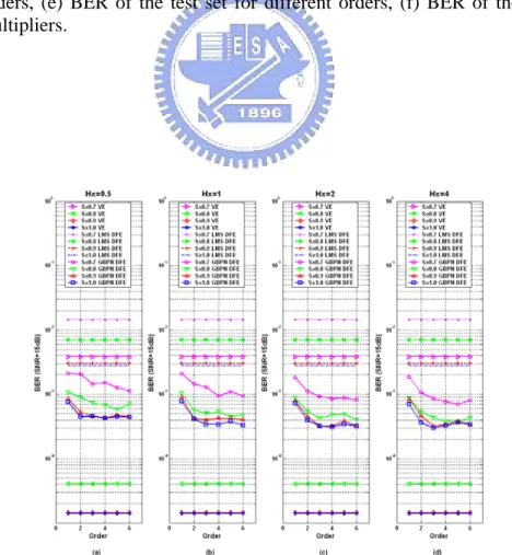
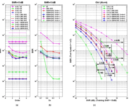
(17) Fig. 3-22: Minimum MSE and standard deviation of MSEs of the evaluation set in Channel 1 at SNR=15dB.. 56. Fig. 3-23: BER of the evaluation set and the test set in Channel 1 at 57. SNR=15dB. Fig. 3-24: BER performance for different levels of the nonlinearity with different hidden neuron multipliers in Channel 1 at SNR=15dB.. 57. Fig. 3-25: Channel 1 test results.. 58. Fig. 3-26: Channel 2 test results.. 58. Fig. 3-27: Channel 3 test results.. 59. Fig. 3-28: Channel 4 test results.. 59. Fig. 3-29: Channel 5 test results.. 60. Fig. 3-30: Channel 6 test results.. 60. Fig. 3-31: Channel 7 test results.. 61. Fig. 4-1: Equivalent model for the band-limited channels with co-channel interference.. 66. Fig. 4-2: Frequency responses of the ISI and the CCI responses.. 67. Fig. 4-3: MIMO MLP/BP-based DFEs.. 68. Fig. 4-4: BER vs. SNR for different types of equalizers in the band-limited channels with co-channel interference at SIR=10, 15 and 20dB.. -xv-. 72.

(18) Fig. 4-5: BER vs. SIR for different types of equalizers in the band-limited channels with co-channel interference at SNR= 15 and 20dB.. 72. Fig. 4-6: BER performance under SIR=15dB, 17.5dB, and 20dB for different ADC resolution at SNR=15dB, 17.5dB, and 20dB.. 74. Fig. 4-7: BER performance vs. SNR for different ADC resolution at 75. SIR=15dB, 17.5dB, and 20dB.. Fig. 4-8: BER performance under SIR=15dB, 17.5dB, and 20dB for different ADC resolution with internal resolution enhancement technique at SNR=20dB.. 77. Fig. 4-9: BER performance vs. SNR with different ADC resolution and different internal resolution at SIR=15dB, 17.5dB, and 20dB.. 78. Fig. 4-10: BER performance vs. SNR for the LMS DFEs and MIMO MLP/BP-based DFEs at SIR=15.0dB, 17.5dB, and 20.0dB.. Fig. 4-11: The MIMO generalized MLP/BP-based DFEs.. 79. 83. Fig. 4-12: BER vs. SNR for different types of equalizers in the wireline band-limited channels with co-channel interference at SIR=10, 15 and 20dB.. 85. Fig. 4-13: BER vs. SIR for different types of equalizers in the wireline band-limited channels with co-channel interference at SNR= 15 and 20dB.. 87. Fig. 5-1: System Diagram.. 90. Fig. 5-2: The Equivalent Model for the Multi-path Fading Channels.. 91. -xvi-.

(19) Fig. 5-3: Channel Responses of Multi-path Fading Channels.. 92. Fig. 5-4: Frequency Responses of Multi-path Fading Channels.. 92. Fig. 5-5: MLP/BP-based Soft DFEs for Wireless Applications.. 95. Fig. 5-6: PER Performance for different types of equalizers when packet data length is equal to 103.. 100. Fig. 5-7: PER Performance for different types of equalizers when packet data length is equal to 8×103.. 100. Fig. 5-8: PER Performance for different types of equalizers with different packet data length at Eb/N0 = 7.5dB and 10.0dB.. 101. Fig. 5-9: BER Performance for different types of equalizers when packet data length is equal to 103.. 101. Fig. 5-10: BER Performance for different types of equalizers when packet data length is equal to 8×103.. 102. Fig. 5-11: BER Performance for different types of equalizers with different packet data lengths at Eb/N0 = 7.5dB and 10dB.. -xvii-. 102.

(20) -xviii-.

(21) CHAPTER 1 Introduction. 1-1. Thesis Motivation In a digital communication system, the source signal is transmitted over an. intersymbol interference (ISI) channel, corrupted by noise, and then received as a distorted signal. In most cases, the additive white Gaussian noise (AWGN) can be used to model the background noise; however, the noise includes not only ISI and AWGN but the nonlinear distortion as well. If the channel response introduces both intersymbol interference and nonlinear distortions, transmitted signal will be corrupted nonlinearly, leading to worse performance. For example, the saturation of non-ideal amplifier and automatic gain control (AGC) loss in transceivers will produce nonlinear distortions that further degrade the performance of equalizers. Therefore, it is necessary to apply data equalizers to recover the original waveform from the distorted one in practical communication systems [1], [2]. A good equalization design can enhance the whole system performance with an acceptable cost. Conventionally, the NRZ signal recovery is based on either linear equalizers (LEs). -1-.

(22) [1], [3], or decision feedback equalizers (DFEs) [1], [2], [3]. A linear equalizer can restore the original transmitted signal in a wireline band-limited channel, where the channel distortion is linear without spectral nulls in the channel frequency response. Nevertheless, as the channel frequency response has spectral nulls, the received noise will be enhanced in the process of compensating these nulls, resulting in degraded performance. For linear equalization scheme, such channels that lead to malfunctions of equalizers have been termed “severe” ISI channels [4]. The decision feedback equalizer employing previous decisions to remove the ISI on the current symbol has been extensively exploited to serve intersymbol interference rejection. The least mean squares (LMS) algorithm is used to estimate the coefficients of the equalizer [1], [2], [3] whose accuracy determines the system performance. For wireline high data rate applications, timing uncertainly degrades the system performance [5]. The channel response variance that is caused by manufacturing deviation makes the worse situation. It is necessary that using an equalizer to overcome clock skew and channel response variance. In addition, interconnect paths of parallel data I/O would cause the co-channel interference (CCI) [6]. The transmitted signals are tainted by the intersymbol interference that caused by the band-limited channel, the co-channel interference that caused by crosstalk between different channels, and background white noise. For recover the distorted data as well as suppress ISI, CCI and AWGN, a multi-input multi-output (MIMO) channel equalizer is essential. Error control codes (ECC) are applied to enhance the accuracy of the transmitted data in wireless applications. The channel decoder with soft information inputs is widely employed to improve the error correction capability [7], and the bit interleaving is included [8] in wireless fading channels. With the soft output [9] and soft feedback [10] channel equalizers, the soft decision channel decoder will receive more information from. -2-.

(23) the channel and therefore precisely decode the data sequence, leading to better BER performance. Besides, the equalization schemes can be thought of a mapping from the received waveform to the transmitted data. The pattern recognition techniques have been used to identify the severely distorting date. Having the capability of classifying the sampling pattern and fault tolerance, artificial neural networks are very suitable for the channel equalizations. Recently, various equalizer designs based on artificial neural networks have been studied to the severely distorting signal recoveries [11]. Neural-based approaches have more flexibility and better performance than conventional equalization techniques. The proposed approaches are based on the most popular multi-layer perceptron neural network with backpropagation algorithm (MLP/BP) [12], [13], [14], [15], [16]. As well, the MLP architecture can be regarded as a separateness-summation modus operandi in separating pattern space. For wireline applications, we apply the MLP/BP-based channel equalization schemes to different applications. In the wireline band-limited channel that the data rate is ten times as much as the channel bandwidth, the MLP/BP-based feedforward equalizer (FFE) can recover the distorted data [17]. The MLP/BP-based DFE provide better performance, tolerate sampling clock skew, and permit channel response variance [18]. In wireline parallel I/O channels, the MIMO MLP/BP-based DFE can suppress ISI, CCI and AWGN, simultaneously [19]. However, the traditional MLP/BP-based DFEs are not good enough for the severe ISI channels with nonlinear distortions. We present a new neural network model, which is based on the MLP/BP neural network. This model utilizes a multivariate power series for the summation function of the MLP/BP neural networks [20], [21]. The corresponding training algorithm is deduced by the gradient steepest descent method; consequently, the convergence solutions exist. Compared to the conventional approach. -3-.

(24) using a first order multivariate polynomial, the boundaries separating the pattern space change from piecewise linear into piecewise nonlinear. Therefore, this novel model is a generalized MLP/BP neural network (GMLP/BP) that is more flexible than other piecewise linear approaches because of the nonlinear separating pattern space. In such channels, the GMLP/BP-based DFE can outperform the traditional MLP/BP-based equalization schemes [22]. Also, the performance of the MIMO GMLP/BP-based DFE is better than that of the MIMO MLP/BP-based DFE in wireline parallel channels that contain ISI, CCI, and background white noise [23]. For wireless applications, a modified approach, which is also based on the most popular MLP/BP neural network, is presented. We apply the soft output and the soft decision feedback structure to the MLP/BP-based channel equalizer that concatenates with the soft decision channel decoder to improve whole performance on multi-path fading channels. Moreover, the performance of the MLP/BP-based soft DFE is also increased with the optimal scaling factor searching of the transfer function in the output layer of the MLP/BP neural networks and extra small random disturbances added to the training data [24].. 1-2 Paper Survey There are various channel equalization schemes that are applied to different channel conditions. We survey the representative equalization approaches for wireline and wireless communications in these few years. These papers treat of different channel equalization schemes for wireline band-limited channels, wireline severe ISI channels, and wireless fading channels, respectively. The linear equalizers can recover the distorted data in wireline band-limited channels -4-.

(25) [1], [2], [3]. For wireline severe ISI channels or wireless fading channels, the linear equalization schemes are unsuitable [4], [5]. In serve ISI channels, the DFEs [1], [2], [3], [5] can avoid the influence of the spectral nulls and outperform the LEs. For wireline high data rate communications, DFEs are applied to improve the data rate or reduce the error rate [25], [26], [27]. In practice circuits, the channel responses of different interconnect paths of parallel data I/O are different. The receiver must tolerate channel responses variance and sampling clock skew. Besides, CCI makes the problem more severely. The most popular training algorithm of DFEs is the least mean squares (LMS) algorithm, which is a minimum mean square error (MMSE) solution. One of the great methods for improving DFEs, support vector machines (SVM) based DFEs [28], [29], [30] uses the minimum bit error rate (MBER) solution instead of the MMSE solution to enhance system performance, but requires the estimation of channel impulse response (CIR) to compute the weighting vectors. Although the performance of SVM DFE is better than LMS DFE, the complexity of SVM DFE is much higher due to the additional channel estimator. The Viterbi Equalizer (VE) [31] that requires CIR estimation can also be used in severe ISI channels and achieve much better performance. However, the accuracy of CIR dominates the performance particularly, and a nonlinear distortion of received signal will cause significant performance degradation to VE. Because feed-forward neural network based channel equalization schemes are the most suitable architectures for very large-scale integration (VLSI) implementation, we survey the several well-liked neural network models that contain single layer perceptron (SLP) neural networks [13], [14], [16], polynomial perceptron (PP) neural network [14], [16], functional-link (FL) neural networks [14], [16], [32], radial basis function (RBF). -5-.

(26) neural networks [14], [15], [16], counterpropagation (CP) neural networks [14], [16], [33], and MLP/BP neural networks [12], [13], [14], [15], [16]. The single layer perceptron neural network is the simplest neural network model, but it can’t solve the linear non-separable problem. In wireline applications, SLP-based channel equalizers [34] are better than LMS-based linear equalizers. The polynomial perceptron neural network uses a polynomial function to represent the input data and then a SLP neural network to combine these represented data and generate the output. By the input data represented, PP neural networks can solve linear non-separable problems. In severe ISI channels, PPNN-based channel equalizers outperform linear equalizers [35]. In multi-path fading channels, PPNN-based channel equalizers can suppress ISI and CCI [36], [37], simultaneously. The complexity of the PPNN-based channel equalization schemes is depended on tap number and polynomial degree. Based on the same concept, the functional-link neural networks are proposed. The higher-order input terms of the FL neural networks can be generated by the expanded functions, which comprise polynomial functions, trigonometric functions, signum functions and other nonlinear functions. The PP neural network is a special case of FL neural network. In severe ISI channels, FLNN-based channel equalizers can recover severe distorted data [38], [39], [40]. In multi-path fading channels, FLNN-based channel equalizers can suppress ISI and CCI with better performance than LEs and DFEs [41], [42], [43]. Excluding above definitely defined functions, a set of radial basis functions, which paves the input space with overlapping receptive fields, can be taken as the functional expander of the RBF neural networks. The most frequently used radial basis function is the Gaussian function. The output of the radial basis function is maximized by minimized. -6-.

(27) the Euclidean distance between the input vector and the centroid. To find the correct centers of the radial basis functions is very important. Thus, the clustering technique is the key issue [44]. The RBF-based channel equalization schemes [45], [46], [47], [48], [49] can be applied to wireline band-limited channels, severe ISI channels with or without nonlinearity, severe ISI channels with CCI, and wireless fading channels. Overall, the architecture of PP neural networks, FL neural networks, and RBF neural networks consists of two main parts, the functional expander and the linear combiner. The functional expander, which performs nonlinear mapping for the input data, and make the linear non-separable problem become linear separable. Afterward, a SLP neural network, which is trained by the simple delta-learning rule, is taken as the linear combiner to associate the represented input data with the desired outputs. The pattern space separating boundaries of such neural networks are nonlinear. The counterpropagation neural network is two-layer structure. The first layer is a winner-take-all network, and the second layer is perceptron-based architecture. The learning speed of CP neural networks is faster than MLP/BP neural networks, but the accuracy is worse. The CP-based channel equalizers outperform LEs under nonlinear channel characteristics [50]. Since late 1980s, the MLP/BP neural network is the most important and most popular neural network model [12], [13], [14], [15], [16]. The MLP neural network can be regarded as a separateness-summation modus operandi. Because the summation function of the MLP/BP neural network is a first order multivariable polynomial function, the boundaries of neighbors are linear or piecewise linear. Also, it is treated as continuous linear mapping processes. In severe ISI channels, the MLP/BP-based feedforward equalizers [51], [52], and the MLP/BP-based decision feedback equalizers [53], [54], [55] have been widely used to. -7-.

(28) distorted signal recovery. The MLP/BP neural network combined decoder and equalizer [4] merges forward equalization and data decoder in an MLP/BP neural network. It can offer higher system integration and better performance than the traditional separate solutions. The MLP/BP DFE with lattice filter [56] uses a lattice filter to whiten its input signal. The lattice filter can reject a quantity of the noise and make the signal clear. The convergence rate of the neural network, the steady state mean square error, and the bit error rate of whole system can be improved in chorus. For constant envelope signal processing, we can separate in-phase and quadrature-phase components and then the real-value activation functions can handle this problem. Besides, there are two main approaches for the development of a complex neural network. One looks for fully complex activation function [57], [58], and has been applied to distorted QPSK signal recovery [59]. Another has used split complex activation function [60], [61], and has been also employed to channel equalization [62]. For wireless communications, the MLP/BP-based DFEs are applied to indoor radio channels [63] and digital satellite channels [64]. In wireless applications, the length of the training symbols and the number of the training epochs are sternly limited. As well, the MLP/BP-based DFEs can be used to suppress not only ISI but also CCI that is due to other co-channel users [65], [66]. The MLP neural network with hierarchical backpropagation algorithm (HBP) combines the hierarchical approach and BP algorithm [67]. It can solve some problems of the local minimum in the BP algorithm and improve the system performance. Except MMSE based learning rule, the least relative entropy (LRE) [68], [69] based learning algorithm has been applied to SLP neural network based equalizers and MLP neural network based equalizers. The dynamics of the LRE based algorithm is better than that of the MMSE based learning rule. It means that the learning speed of the LRE based. -8-.

(29) algorithm is faster than the MMSE based one. Moreover, neural networks can be trained by fuzzy if-then rules [16]. For nonlinear channel equalization applications, an adaptive neural fuzzy filter provides good performance [70].. 1-3 Thesis Organization The rest of this thesis is organized as follows. The traditional MLP/BP neural networks and the generalized MLP/BP neural networks are first addressed in chapter 2. The detail of proposed neural-based channel equalization schemes for wireline SISO applications, wireline MIMO applications, and wireless applications are described in chapters 3, 4, and 5, respectively. Some conclusions and future works of the proposed methods are made in chapter 6. Brief description of each chapter is given below:. y In chapter 2, the brief review of the multi-layer perceptron neural networks with backpropagation algorithm is introduced at first. Subsequently, the generalized multi-layer perceptron neural networks and corresponding backpropagation algorithm is proposed. At last, the comparison of computational complexity is made. y In chapter 3, the MLP/BP-based DFEs with high skew tolerance for wireline band-limited channels are presented at the beginning. Afterward, the generalized MLP/BP-based DFEs for wireline severe ISI channels are proposed. y In chapter 4, the MIMO MLP/BP-based DFEs and the MIMO generalized MLP/BP-based DFEs for overcoming ISI and CCI in wireline band-limited channels are given. -9-.

(30) y In chapter 5, the MLP/BP-based soft decision feedback equalizers for wireless communications are delivered. y In chapter 6, some concluding remarks will be derived from this research. Then briefly discussions illustrate our research activities in the future.. -10-.

(31) CHAPTER 2 Generalized MLP/BP Neural Networks. Artificial neural networks are systems that are deliberately constructed to make use of some organizational principles resembling those of the human brain. In 1943, McCulloch and Pitts proposed a simple mathematical model of the biological neuron, usually called an M-P neuron. The generalizations or variations of the M-P neuron are the basic component of artificial neural networks. An artificial neural network consists of a set of highly interconnected neurons such that each neuron output is connected to other ones or/and to itself through weights, which with or without lag. In 1957, Rosenblatt created the perceptron neural networks that include single-layer feedforward networks, which without hidden layers; and multi-layer feedforward networks, which with a hidden layer or more. But there is no suitable training algorithm for multi-layer perceptron neural networks until the backpropagation algorithm [12] had been proposed. Today, there are many different artificial neural networks had been proposed, but the multi-layer perceptron neural network with backpropagation algorithm is the most important and most popular one [13], [14], [15], [16]. In this work, we treat the MLP/BP neural network model and make a key -11-.

(32) modification to offer a new approach, the generalized MLP/BP neural network. At the beginning of this chapter, we make a review for the traditional MLP/BP neural network. Afterward, a detail arrangement of the generalized MLP/BP neural network is given.. 2-1 Traditional MLP/BP Neural Networks Although the MLP neural network had been treated in late 1950s, the suitable training algorithm wasn’t appeared until the backpropagation algorithm [12] presented. Bryson and Ho in 1969, Werbos in 1974, LeCun in 1985, Parker in 1985, and Rumelhart in 1986 proposed the backpropagation algorithm. The most influential publication of the backpropagation algorithm is Rumelhart’s contribution. Since late 1980s, the MLP/BP neural network has been widely used to pattern recognition, and signal processing [13], [14], [15], [16]. In this section, we treat the MLP/BP neural network because it is the basis of our proposed model. At first, we show the detail of the MLP neural network architecture. Subsequently, the deduced process of the backpropagation algorithm is presented.. 2-1-1. Architecture. The architecture of a multi-layer perceptron neural network [12], [13], [14], [15], [16] is shown in Fig. 2-1. The neurons are arranged into several layers. The first layer is the input layer, the final layer is the output layer, and other in-between layers are hidden layers. The neuron number of each layer could be singular form or plural form. In the input layer, each neuron includes a single input and a single output. In other layers, there -12-.

(33) are several inputs and one output in each neuron. The different neurons, which situate in neighbor layers, connect together through respective weights without lag. A neuron, the processing unit, of the MLP neural networks [12], [14], [16] is shown in Fig. 2-2. The output of a neuron is the value obtained from applying a transfer function to a weighted sum of its inputs, where each input is the output of a neuron situated in the previous layer. The weighted sum of the inputs can be described as a first order polynomial function. As well, commonly used transfer functions include hard limit functions (step functions), ramp functions (linear functions), unipolar sigmoid functions (log-sigmoid functions), bipolar sigmoid functions (tan-sigmoid functions), and so on. For different purposes, we can select dissimilar transfer functions to meet the requirement or constraint. In this work, we choose the unipolar sigmoid function as the transfer function of a neuron.. Input Layer. Output Layer Hidden Layer. Fig. 2-1: MLP Neural Network Architecture.. -13-.

(34) [A(n-1)1] [A(n-1)2] Ｗj1 Ｗj2. [A(n-1)i]. Σ. Ｗji. f(.). Anj. Ｗjn. [A(n-1)n]. Fig. 2-2: Neuron of MLP Neural Networks.. 2-1-2 Backpropagation Algorithm The MLP/BP neural networks are supervised learning. It means that a training set includes an input vector and a desired output vector. Using the MLP/BP neural networks to solve problems includes two phases, one is training procedure and another is testing procedure. In the training phase, we base on the gradient steepest descent method to minimize the error function for updating the weights. After that we apply the training result to obtain the network response in testing phase. Now, a mathematical description of backpropagation algorithm [12], [15] is shown as follows:. Output = Anj = f(net nj ) ,. (2-1). where Anj is the output of neuron j in the n-th layer, f(.) is the transfer function obtaining the output of a neuron, and netnj is the output of the summation function of neuron j in the n-th layer. Furthermore,. net nj = Summation _ Function = ∑ W ji A( n −1)i − θ j ,. (2-2). j. where Wji represents the weight of the connection between neuron j in the n-th layer and neuron i in the (n-1)-th layer, and θj is the threshold (bias) of neuron j. The Wjim should be -14-.

(35) trained to minimize the error function E = Error _ Function =. 1 ⋅ ∑ (T j − Anj ) 2 , 2 j. (2-3). where Tj is the desired output of neuron j in the output layer. By the gradient steepest descent method, the error function (2-3) can be minimized by ΔW ji = −η ⋅. ∂E , ∂W ji. (2-4). the update quantity for Wji, and η is the learning rate. By chain rule,. For. ∂E ∂E ∂netnj = ⋅ , ∂W ji ∂netnj ∂W ji. (2-5). ∂E ∂E ∂Anj ∂netnj = ⋅ ⋅ , ∂W ji ∂Anj ∂netnj ∂W ji. (2-6). ∂netnj ∂ = (∑ W ⋅ A − θ j ) = A( n -1)i , ∂W ji ∂W ji k ji ( n −1) k. (2-7). ∂Anj ∂ = ⋅ f (netnj ) = f ' (netnj ) . ∂netnj ∂netnj. (2-8). ∂E , there are two cases that should be discussed: ∂Anj. (1) When the n-th layer is the output layer, 2 ∂E ∂ 1 = [ ⋅ ∑ (Tk − Ank ) ] = −(T j − Anj ) . ∂Anj ∂Anj 2 k. (2-9). (2) When the n-th layer is a hidden layer,. ∂net( n +1) k ∂E ∂E = ∑( )⋅( ) ∂Anj ∂net( n +1) k ∂Anj k = ∑( k. = ∑( k. ∂E ∂net( n+1) k ∂E ∂net( n+1) k. ) ⋅[. ∂ ∂A. (∑Wki ⋅ Ani - θ k )] . nj. i. ) ⋅ Wkj -15-. (2-10).

(36) Let. ∂E ∂net nk. = −δ nk be the error signal of neuron k in n-th layer,. ∂E ∂net( n +1) k. = −δ ( n +1) k can. be deduced and (2-10) can be rewritten as. ∂E = −∑ δ ( n +1) k ⋅ Wkj . ∂Anj k. (2-11). Furthermore, according to (2-7), the deviation in (2-5) can be rewritten as. ∂E = −δ nj ⋅ A( n −1) i . ∂W ji. (2-12). By (4) and (12), ΔW ji = −η ⋅. ∂E = η ⋅ δ nj ⋅ A( n −1)i . ∂W ji. (2-13). Similarly, the following equation can be obtained. Δθ j = − η ⋅ δnj ,. (2-14). where Δθj is the update quantity of θj. From the above deductions, there are two possible cases: (1) If W ji is between the output layer and its anterior layer (a hidden layer), (2-7), (2-8), and (2-9) can be applied to (2-6),. ∂E = −(T j − Anj ) ⋅ f ' (netnj ) ⋅ A( n −1)i . ∂W ji. (2-15). After comparing (2-12) and (2-15), we can obtain. δnj = (T j − Anj ) ⋅ f ' (net nj ). (for output layer).. (2-16). (2) If W ji is between a hidden layer and its anterior layer (a hidden layer or the input layer), (2-7), (2-8), and (2-11) can be applied to (2-6),. ∂E = [ −∑ δ ( n +1) k ⋅ Wkj ] ⋅ f ' ( netnj ) ⋅ A( n −1) i . ∂W ji k. (2-17). The following equation can be obtained from comparing equations (2-12) and (2-17) -16-.

(37) δnj = [∑ δ( n +1) k ⋅ Wkj ] ⋅ f ' (netnj ). (for hidden layer).. (2-18). k. In this work, a unipolar sigmoid function is used to the transfer function of a neuron. The first derivative of the unipolar sigmoid function can be represented as the terms of itself, as shown in (2-19) and (2-20).. f (netnj ) =. 1 , − net 1 + e nj. f ' (netnj ) =. e nj 1 1 = ⋅ (1 − ) −netnj 2 −netnj −net 1 + e nj (1 + e ) 1 + e. (2-19). − net. = f ( net nj ) ⋅ [1 − f (net nj )] = Anj ⋅ (1 − Anj ) ,. (2-20). By such representation, (2-16) and (2-18) can be rewritten as (2-21) and (2-22).. δ nj = (T j − Anj ) ⋅ Anj ⋅ (1 − Anj ). (for output layer),. δ nj = [∑ δ ( n +1) k ⋅ Wkj ] ⋅ Anj ⋅ (1 − Anj ). (for hidden layer).. (2-21) (2-22). k. In each iteration, the weights and thresholds are updated. When the whole set of training data has been cycled once, calculate mean square error (MSE) of this training epoch. We repeat such epoch and record the best result, which consists of weights and thresholds and leads to the minimal MSE among past training epochs. Check whether the current MSE is smaller than the maximum tolerable error, which the result meets the training object, and the entire training epochs have been completed, which stands for the maximum patient training time. If the alternative conditions have been reached, the training process is terminated. At this moment, the training result is harvested. In general, reduce training time and enhance system performance are certain exclusive property. [14], [15], [16]. -17-.

(38) Because the MLP/BP neural network is an MMSE approach, the training results will converge on local optima. Using different network configurations, different initial condition and different learning rate, will conduce to different performance [13], [14], [16]. In general, could perform quite a few independent training runs and choose the most suitable result as the final solution. Moreover, the MLP/BP neural network can be regarded as a separateness-summation modus operandi in separating pattern space. Because the summation function of the MLP/BP neural network is linear, the boundaries of neighbors are linear or piecewise linear. [14], [16] For a complex system, the number of neurons should increase for better approximation.. 2-2 Generalized MLP/BP Neural Networks To achieve more flexibility and better performance, a multivariate power series is used to replace a first order multivariate polynomial as the summation function of the MLP/BP neural networks, leading to a significant modification for the traditional MLP/BP neural network. Therefore, regarded as a general form of the MLP/BP neural network, the proposed model can be termed as a generalized MLP/BP neural network. This key modification comes from the previous study of speech recognition where a better performance can be attained by using the multivariate power series [20], [21]. In this work, this new method is applied to the waveform equalization and results in a significant improvement in performance. In this section, we show the architecture of the generalized MLP/BP neural network at first. Subsequently, the deduced process of the corresponding backpropagation algorithm is presented. Referring to the traditional MLP/BP neural network and the -18-.

(39) generalized MLP/BP neural network, we find that the traditional method is a special case of the proposed model.. 2-2-1 Architecture The network architecture of our proposition is the same as the traditional MLP/BP neural networks. That has been shown in Fig. 2-1. However, the construction of neurons of the both is different. A neuron of this new approach is shown in Fig. 2-3. The output of a neuron of the proposed scheme is the value obtained from applying a transfer function to a weighted sum of the power terms of its inputs, where each input is the output of a neuron situated in the previous layer. The weighted sum of the power terms of the inputs can be represented as a multivariate power series. On the other word, the summation function of the generalized MLP/BP neural networks is a multivariate power series that substitute for the first order multivariate polynomial. Similarly, we can select dissimilar transfer functions to meet the requirements of different purposes.. [A(n-1)1]1 [A(n-1)1]2 Ｗj11 Ｗj12. [A(n-1)i]1. Ｗjil. Σ. f(.). Ｗjnm. [A(n-1)n]m. Fig. 2-3: Neuron of Generalized MLP/BP Neural Networks.. -19-. Anj.

(40) 2-2-2 Corresponding Backpropagation Algorithm In this subsection, we present the training algorithm for the generalized MLP/BP neural network. It is similar to the traditional training algorithm. Diversely, the multivariate power series is used to replace the first order multivariate polynomial as the summation function of the MLP/BP neural networks. The corresponding backpropagation algorithm of the proposed approach is deduced by the gradient steepest descent method and is shown as follows:. Output = Anj = f (netnj ) ,. (2-1). where Anj is the output of neuron j in the n-th layer, f(.) is the transfer function obtaining the output of a neuron, and netnj is the output of the summation function of neuron j in the. n-th layer. Furthermore, net nj = Summation_Function = ∑∑W jim A(mn −1) i − θ j , i. (2-23). m. where m is the order of the summation function, Wjim represents the weight of the connection between neuron j in the n-th layer and neuron i in the (n-1)-th layer corresponding to order m, and θj is the threshold (bias) of neuron j. The Wjim should be trained to minimize the error function. E = Error _ Function =. 1 ⋅ ∑ (T j − Anj ) 2 , 2 j. (2-3). where Tj is the desired output of neuron j in the output layer. By the gradient steepest descent method, the error function (2-3) can be minimized by ΔW jim = −η ⋅. ∂E ∂W jim. ,. (2-24). the update quantity for Wjim, and η is the learning rate. By chain rule,. -20-.

(41) ∂E ∂W jim ∂E ∂W jim. For. ∂E. =. ∂netnj. ⋅. ∂netnj , ∂W jim. (2-25). ∂E ∂Anj ∂netnj ⋅ ⋅ , ∂Anj ∂netnj ∂W jim. =. (2-26). p ∂netnj ∂ = [∑∑ W jim ⋅ A(mn −1) k − θ j ] = A(mn -1)i , ∂W jim ∂W jim k m =1. (2-27). ∂Anj ∂ = ⋅ f (netnj ) = f ' (netnj ) . ∂netnj ∂netnj. (2-28). ∂E , there are two cases that should be discussed: ∂Anj. (1) When the n-th layer is the output layer, 2 ∂E ∂ 1 = [ ⋅ ∑ (Tk − Ank ) ] = −(T j − Anj ) . ∂Anj ∂Anj 2 k. (2-29). (2) When the n-th layer is a hidden layer,. ∂net( n +1) k ∂E ∂E = ∑( )⋅( ) ∂Anj ∂net( n +1) k ∂Anj k = ∑( k. = ∑( k. Let. ∂E ∂net nk. ∂E ∂net( n+1) k ∂E ∂net( n+1) k. ) ⋅[. ∂ ∂A. p. (∑∑ Wkim ⋅ Anim - θ k )] . nj. i. (2-30). m=1. p. ) ⋅ [∑ m ⋅ Wkjm ⋅ Anj( m −1) ] m =1. = −δ nk be the error signal of neuron k in n-th layer,. ∂E ∂net( n +1) k. = −δ ( n +1) k can. be deduced and (2-30) can be rewritten as p ∂E = −∑ δ ( n +1) k ⋅ [∑ m ⋅ Wkjm ⋅ Anj( m −1) ] . ∂Anj k m =1. (2-31). Furthermore, according to (2-27), the deviation in (2-25) can be rewritten as. ∂E ∂W jim. = −δ nj ⋅ A(mn −1)i .. (2-32). -21-.

(42) By (2-24) and (2-32), ΔW jim = −η ⋅. ∂E ∂W jim. = η ⋅ δ nj ⋅ A(mn −1) i .. (2-33). Similarly, the following equation can be obtained Δθ j = − η ⋅ δnj ,. (2-34). where Δθj is the update quantity of θj. From the above deductions, there are two possible cases: (1) If W jim is between the output layer and its anterior layer (a hidden layer), (2-27), (2-28), and (2-29) can be applied to (2-26),. ∂E ∂W jim. = −(T j − Anj ) ⋅ f ' (netnj ) ⋅ A(mn −1) i .. (2-35). After comparing (2-32) and (2-35), we can obtain. δnj = (T j − Anj ) ⋅ f ' (net nj ). (for output layer).. (2-36). (2) If W jim is between a hidden layer and its anterior layer (a hidden layer or the input layer), (2-27), (2-28), and (2-31) can be applied to (2-26),. ∂E ∂W jim. p. = [−∑ δ ( n +1) k ⋅ (∑ m ⋅Wkjm ⋅ Anj( m −1) )] ⋅ f ' (netnj ) ⋅ A(mn −1) i .. (2-37). m =1. k. The following equation can be obtained from comparing equations (2-32) and (2-37) p. δnj = [∑ δ( n +1) k ⋅ ∑ m ⋅ Wkjm ⋅ Anj( m −1) ] ⋅ f ' (netnj ) k. (for hidden layer).. (2-38). m =1. In this work, a unipolar sigmoid function is used to the transfer function of a neuron. The first derivative of the unipolar sigmoid function can be represented as the terms of itself, as shown in (2-19) and (2-20). f (netnj ) =. 1 , − net 1 + e nj. (2-19) -22-.

(43) − net. e nj 1 1 = ⋅ (1 − ) f ' (netnj ) = −netnj 2 −netnj −net 1 + e nj (1 + e ) 1 + e = f (netnj ) ⋅ [1 − f (netnj )] = Anj ⋅ (1 − Anj ) ,. (2-20). By such representation, (2-36) and (2-38) can be rewritten as (2-39) and (2-40).. δ nj = (T j − Anj ) ⋅ Anj ⋅ (1 − Anj ). (for output layer),. (2-39). p. δ nj = [∑ δ ( n +1) k ⋅ (∑ m ⋅ Wkjm ⋅ Anj( m −1) )] ⋅ Anj ⋅ (1 − Anj ) k. (for hidden layer).. (2-40). m =1. Referring to the traditional MLP/BP neural network and the generalized MLP/BP neural network, we make comparisons between (2-16) and (2-36); (2-18) and (2-38); (2-21) and (2-39); (2-22) and (2-40). The generalized MLP/BP neural network is actually equivalent to the traditional MLP/BP neural network when m=1, indicating that the traditional method is a special case of the proposed model. Thus the new approach being presented is a generalized model. Moreover, the network configuration of this scheme has more degrees of freedom than the traditional one. Because the summation function of the GMLP/BP neural networks is a multivariate power series (nonlinear function), the boundaries of neighbors become either nonlinear or piecewise nonlinear. As the nonlinear summation function within each neuron is materialization in each layer of the GMLP/BP neural networks, the proposed approaches present continuous nonlinear pattern space mapping potential. Theoretically, increases of the summation function order and the number of neurons can achieve better approximation to fit a nonlinear system. Therefore, the proposed scheme will have more flexibility and better performance than traditional MLP/BP neural networks do. Similar to the traditional approach, the training procedure of this GMLP/BP neural network attains different performance by varying initial conditions, learning rates,. -23-.

(44) network parameters or summation function orders. Moreover, designers could perform numerous independent training runs and select the most suitable result as the final solution. Generally, the order of the fitting function is equal to or less than that of the target function. In most cases, the target function is complex or even unknown, and the best fitting function order is determined by experimentation or experience. To simplify the problem, the fitting function order is selected as low as possible while the error is set to be less than the maximum tolerable bound. In general, the order of the most approximation system is equal to or less than three; however, in high performance systems or special applications, the order may be higher. In algebraic, this new approach extends the traditional scheme from the first order approximation to infinity. The most suitable summation function order of this scheme can be determined by computer simulations for different applications.. 2-3 Complexity Analysis Because the order of the neuron of the generalized MLP/BP neural networks is more than one, it is necessary to generate the power terms for the inputs in each layer. In addition, the training algorithm of the generalized MLP/BP neural networks is modified from “generalized delta-learning rule”. The complexity and cost of the generalized MLP/BP neural networks will be higher than the traditional MLP/BP neural networks but the former results in better pattern space separability and better performance. The comparison of computational complexity in terms of additions, multiplications and sigmoid function substitution between the traditional MLP/BP neural networks and the generalized MLP/BP neural networks is shown in Table 2-1. -24-.

(45) Table 2-1: The comparison of computational complexity.. Operation. MLP/BP neural networks (Single Hidden Layer). GMLP/BP neural networks (Single Hidden Layer). Addition. (Ni + 1) · Nh + (Nh + 1) · No. (m · Ni + 1) · Nh + (m · Nh + 1) · No. Multiplication. Ni · Nh + Nh · No. (2m - 1) · Ni · Nh + m · Nh · No. Function Substitution. Nh + No. Nh + No. Notations: Input Neuron Number = Ni Hidden Neuron Number = Nh Output Neuron Number = No Summation Function Order = m. -25-.

(46) -26-.

(47) CHAPTER 3 SISO GMLP/BP-based DFEs for Wireline Applications. For wireline communications, we apply the GMLP/BP-based channel equalization schemes to different applications. In wireline band-limited channels that the data rate is about ten times as much as the channel bandwidth, the traditional MLP/BP-based DFEs provide better performance, tolerate more sampling clock skew, and permit larger channel response variance than LMS DFEs. Because the frequency response of a wireline band-limited channel is without spectral nulls, the high order approximation has no benefit. The first order ones can satisfy the system requirements. However, the traditional MLP/BP-based DFEs are not good enough for the severe ISI channels with nonlinear distortions. The frequency responses of severe ISI channels contain spectral nulls and nonlinear distortions lead to worse situations. In such channels, the generalized MLP/BP-based DFEs can outperform the traditional MLP/BP-based DFEs that do better than the LMS DFEs. This chapter is organized as follows. The traditional MLP/BP-based DFEs with high -27-.

(48) skew tolerance for wireline band-limited channels are presented at the beginning. Afterward, the GMLP/BP-based DFEs for wireline severe ISI channels are proposed.. 3-1 MLP/BP-based DFEs with High Skew Tolerance for Band-limited Channels A traditional MLP/BP neural network is realized as a waveform equalizer for distorted nonreturn-to-zero (NRZ) data recovery in band-limited channels. Moreover, the proposed approach can tolerate sampling clock skew and channel response variance. According to simulation results, the proposed design can recover severe distorted NRZ data with better performance than LMS DFEs in the band-limited channel that the data rate is about ten times as much as the channel bandwidth. Under the 20% channel response variance and the 30% sampling clock skew, the MLP/BP-based DFE can provide an acceptable performance. By fixed-point simulations, the proposed scheme is realizable and outperforms the LMS DFE. Further, the internal resolution enhancement technique provides a better compromise between cost and performance. This section is organized as follows. The system overview is presented in subsection 1 while subsection 2 shows the MLP/BP-based DFEs. Afterward, the simulation results show in subsection 3. Finally, we make a brief summary in subsection 4.. 3-1-1 System Overview In practice circuits of wireline communications, the channel characteristic of different interconnect paths of parallel data I/O channels are different but analogous. -28-.

(49) Besides, sampling clock skew makes the problem more severely. In such conditions, the received signal is deteriorated substantially by intersymbol interference, clock skew and background noise. The system diagram of a single clock source is shown in Fig. 3-1. If the data rate of transmitted signals is higher than the channel capacity, the received signal pulse is unable to complete its transition within a symbol interval. The equivalent model for the wireline band-limited channels is shown in Fig. 3-2 where a finite impulse response (FIR) filter is used to model the ISI channel response with the AWGN as the background noise. The ISI channel response with AWGN can be written as follows:. H(z) = f 0 + f1 ⋅ z −1 + f 2 ⋅ z −2 + ... + f L ⋅ z − L ,. (3-1). L. y k = ∑ f i ⋅ x k −i ,. (3-2). yˆ k = y k + n ,. (3-3). i =0. where H(z) is the transfer function of the ISI channel; L is the length of the channel response; xk is the input sequence; yk is the channel output which is warped by ISI only; nk is the AWGN; ŷk is the received signal which is distorted by both ISI and AWGN. In this work, several wireline band-limited parallel I/O channels that consist of analogous channel responses and different sampling clock skews are used to verify the proposed approaches. Their transfer functions with different F3dB/F ratio are shown in Table 3-1. The frequency responses of these channels are illustrated in Fig. 3-3. These frequency responses are without spectral nulls. Base on foregoing channels, clock skews between +/- 30% are considered to represent a worse situation of the practical wireline high-speed communications.. -29-.

(50) Channel A, Clock Skew A Channel B, Clock Skew B Channel C, Clock Skew C Channel D, Clock Skew D Channel E, Clock Skew E. U1. U2. Clock Generator. Fig. 3-1: System diagram.. AWGN. Tx (2-PAM Signal). Band-limited Channel (First Order RC Low-Pass Filter). Rx X (NRZ Signal). Fig. 3-2: Equivalent model for the band-limited channels.. -30-.

(51) Table 3-1: Transfer functions of several wireline band-limited channels. ID. F3dB/F. Channel Impulse Response. 1. 0.08. [0.3951 0.2390 0.1446 0.0875 0.0529]. 2. 0.09. [0.4319 0.2454 0.1394 0.0792 0.0450]. 3. 0.10. [0.4665 0.2489 0.1328 0.0708 0.0378]. 4. 0.11. [0.4990 0.2500 0.1252 0.0627 0.0314]. 5. 0.12. [0.5295 0.2491 0.1172 0.0551 0.0259]. Fig. 3-3: Frequency responses of several similar wireline band-limited channels.. -31-.

(52) 3-1-2 MLP/BP-based DFEs The block diagram of the MLP/BP-based DFEs is shown in Fig. 3-4. This MLP/BP-based DFE is the single hidden layer MLP architecture. The inputs of the MLP/BP-based DFE consist of feed-forward signals, which come from the input symbols by a tapped-delay-line register, and feedback signals, which come from previous decisions by another tapped-delay-line register. We evaluate different tap numbers in the forward part and the feedback part of the equalization schemes and select the most suitable arrangement. In this work, all equalization schemes have 11 symbols in the forward part and 5 symbols in the feedback part. The number of neurons in the input layer is equal to 16. The MLP/BP-based DFEs uses the single hidden layer MLP architecture. The number of neurons in the hidden layer is 2 times of that in the input layer. Since all the proposed equalization schemes have a single output, the number of neurons in the output layer is equal to 1.. Z-1. Input X-n. Z-1 X-1. Z-1 X0. Z-1 Ym. Xn. Z-1 Y2. Z-1 Y1 Input Layer. Hidden Layer. Output Layer. MLP/BP Neural Network. Threshold. Output. Fig. 3-4: MLP/BP-based DFEs. -32-.

(53) 3-1-3 Simulation Results The performance of the MLP/BP-based DFE is evaluated through the simulations for the distorted NRZ signal recovery in the band-limited channel that the data rate is ten times of the channel bandwidth. In this section, a regular input pattern configuration of the equalization schemes is presented first followed by the modified configuration. At last, the fixed-point simulations and its enhancement are discussed in detail.. 3-1-3-1 Regular Configuration Because the MLP/BP neural networks are supervised learning, a training set includes an input vector and a desired output vector. The training patterns must represent the system characteristic as exact as possible. Suitable training patterns can improve the training quality. In wireline applications, we can select a longer training set to achieve better performance. In the training procedure, the length of the training set is equal to 104 symbols and the total training epochs are 102. The two-phase learning is used with the learning rate of 0.5 when the mean square error of the training set is larger than 10-3, and the learning rate of 0.125, otherwise. When the training epochs exceed eighty percent of the total epochs, the best parameters will be recorded to achieve the lowest mean square error of the training set in the last twenty percent of the training epochs. Hence the steady-state training results can be recognized. In fact, the simulations indicate no unstable problems as all training processes are converged. Because different initial conditions lead to different effects, the non-training evaluation set that has 105 symbols is used to examine the training quality of numerous independent simulation outcomes. After numerous independent training and evaluation. -33-.

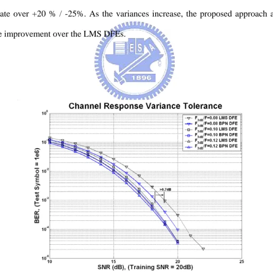
(54) runs, those yielding better outcomes will be chosen to perform a long trial with the test set, and then the best one will be the final test result. We execute fifty independent runs and select the best one as the final result. The length of the test set is 106 symbols, and the evaluation set is a subset of it. At first, we follow the regular input pattern configuration of the equalizers. A band-limited channel (Channel 3) described by the transfer function, H3=0.4665 + 0.2489z-1 + 0.1328z-2 + 0.0708z-3 + 0.0378z-4, is used to estimate the system performance of the LMS DFE and the MLP/BP-based DFE, where the training noise and the evaluation noise are assumed to be SNR=20dB, and SNR of the test signal is between 10dB and 25dB. This channel response indicates that the data rate is ten times of the channel bandwidth. Subsequently, several different band-limited ISI channels (Channels 1, 2, 4, and 5) are used to describe different channel bandwidth vs. data rate ratios that the data rates are eight, nine, eleven, and twelve times the channel bandwidth, respectively. The training result of Channel 3 is applied to these channels, directly. These experiments are used to evaluate the tolerance under different channel response variances. The BER performance for the LMS DFE and the MLP/BP-based DFE in different channels is shown in Fig. 3-5. The proposed approach can outperform the LMS DFE. At last, -30%, -20%, -10%, +10%, +20%, and +30% sampling clock skews are considered, respectively. Similarly, the training result of Channel 3 is applied to these situations, directly. The comparisons of the BER performance for the LMS DFE and the MLP/BP-based DFE in different channels with different clock skews are shown in Fig. 3-6, Fig. 3-7 and Fig. 3-8, respectively. The advantage of the proposed approach can be represented in Fig. 3-9. In view of different channel response variances without sampling clock skew at SNR=20dB, the. -34-.

(55) BER performance of the LMS DFE and the BPN DFE is shown in Fig. 3-9 (a). Considering different clock skews in different channels at SNR=20dB, the comparisons of the BER performance for the LMS DFE and the BPN DFE are shown in Fig. 3-9 (b) to Fig. 3-9(f). From these simulation results, the proposed approach reports better BER performance under +/- 20% channel response variances and +/- 30% sampling clock skews. With F3db/F=0.08 at BER=10-3, the LMS DFE endure about +5% / -8% sampling clock skews and the proposed approach can tolerate over +/- 15%. With F3db/F=0.10, the LMS DFE endure about +13% / -20% and the proposed approach tolerate over +/- 20%. With F3db/F=0.12, the LMS DFE endure about +15% / -25% and the proposed approach tolerate over +20 % / -25%. As the variances increase, the proposed approach achieves more improvement over the LMS DFEs.. Fig. 3-5: BER performance for different types of equalizers in different channels.. -35-.

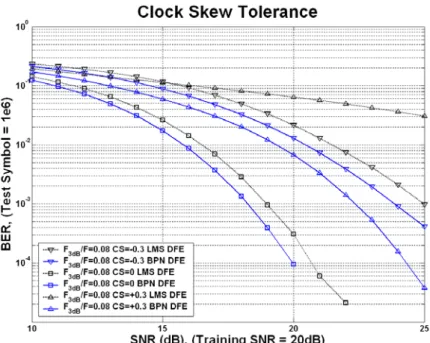
(56) Fig. 3-6: BER performance for different types of equalizers with different clock skews in Channel 1.. Fig. 3-7: BER performance for different types of equalizers with different clock skews in Channel 3.. -36-.

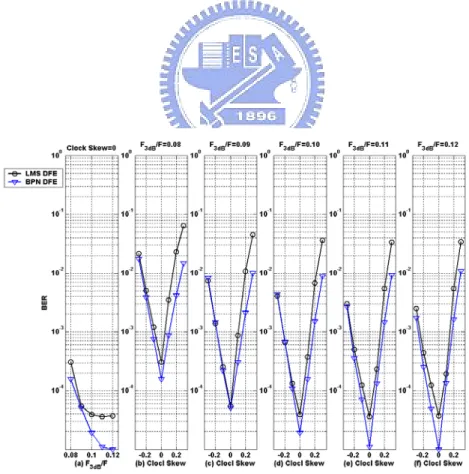
(57) Fig. 3-8: BER performance for different types of equalizers with different clock skews in Channel 5.. Fig. 3-9: BER performance for different channel conditions with regular input pattern configuration at SNR=20dB.. -37-.

(58) 3-1-3-2 Modified Configuration Because the input patterns relate with the training quality and the overall performance, we modify the input pattern configuration that contains more variance by using Channel 1, Channel 3, and Channel 5 with and without +/- 10 percent sampling clock skews to generate the training patterns. By this way, the MLP/BP neural network can provide better fault tolerant capability. The simulation results are shown in Fig. 3-10. From Fig. 3-9 and Fig. 3-10, the modified input pattern configuration can improve the overall performance.. Fig. 3-10: BER performance for different channel conditions with modified input pattern configuration at SNR=20dB.. -38-.

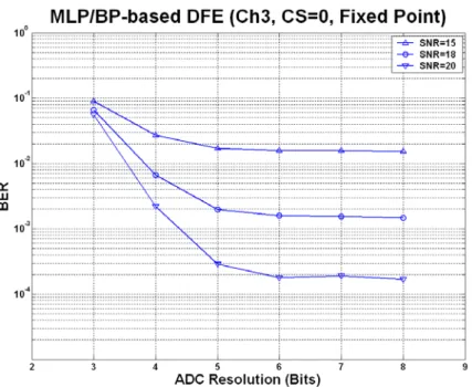
(59) 3-1-3-3 Fixed-Point Simulations In this subsection, the fixed-point simulations and its enhancement of the MLP/BP-based DFE are presented. In general, higher ADC resolution leads to better performance and higher cost. It is a trade-off problem. We consider that added internal resolution to increase the performance under the same ADC resolution. By this way, we can use a lower resolution ADC to replace a higher resolution one and obtain a similar performance. In the fixed-point simulations, we use a hard limiter to replace the log-sigmoid function for low cost consideration. The performance of the MLP/BP neural network should be decreased. The training results of the modified configuration are applied to the fixed-point simulations. The BER performance for different ADC resolution at SNR=15, SNR=18, and SNR=20 are shown in Fig. 3-11. A BER performance comparison with different ADC resolution is shown in Fig. 3-12. The BER performance for different ADC resolution and different internal resolution at SNR=20 are shown in Fig. 3-13. The BER performance for the LMS DFE and the MLP/BP-based DFE in different channels is shown in Fig. 3-14. The fixed-point simulation comparison for the MLP/BP-based DFE in Channel 3 with different clock skews is shown in Fig. 3-15. The BER performance for different channel conditions with modified input pattern configuration under different resolution at SNR=20dB is shown in Fig. 3-16. From Fig. 3-11, the acceptable ADC resolution is five or six bits. From Fig. 3-13, the most suitable combination is five bits ADC with ten bits internal resolution. This internal resolution enhancement technique can provide better performance under the same ADC resolution. In the fixed-point simulations, the performance of the proposed equalizer is better than the LMS DFE. -39-.

(60) Fig. 3-11: BER performance for different ADC resolution at SNR=15, SNR=18, and SNR=20.. Fig. 3-12: BER performance with different ADC resolution.. -40-.

(61) Fig. 3-13: BER performance for different ADC resolution with internal resolution enhancement.. Fig. 3-14: BER performance for different types of equalizers in different channels.. -41-.

(62) Fig. 3-15: BER performance for different types of equalizers with different clock skews in Channel 3.. Fig. 3-16: BER performance for different channel conditions with modified input pattern configuration at SNR=20dB.. -42-.

(63) 3-1-3 Summary The simulation results show that the proposed approach reports better BER performance under +/- 20% channel response variances with +/- 30% sampling clock skews in the band-limited channels that the data rate is about ten times of the channel bandwidth. With different channel responses at BER=10-3, the comparison of sampling clock skew tolerance between the LMS DFEs and the MLP/BP-based DFEs is shown in Tab. 3-2. Because the proposed approach can tolerate more clock skews and large channel response variances, the clock tree design and data interconnection planning can be simplified. For low cost considerations, we can use a preset equalizer to replace an adaptive one. In the fixed-point simulations, the proposed equalizer is realizable and outperforms the LMS DFE. Further, the internal resolution enhancement technique makes the proposed scheme with a better compromise between cost and performance. By the fixed-point simulations, the most suitable combination is five bits ADC with ten bits internal wordlength. However, the performance of the traditional MLP/BP-based DFEs is not good enough for the severe ISI channels with nonlinear distortions. The frequency responses of severe ISI channels contain spectral nulls and nonlinear distortions lead to worse situations. For such channels, we propose the generalized MLP/BP-based DFEs for better performance and show the details in next section.. -43-.

(64) Table 3-2: The comparison of sampling clock skew tolerance. ID. F3dB/F. LMS DFEs. MLP/BP-based DFEs. 1. 0.08. +5% / -8%. +11% / -12%. 2. 0.09. +11% / -18%. +17% / -18%. 3. 0.10. +13% / -20%. +20% / -20%. 4. 0.11. +14% / -22%. +20% / -23%. 5. 0.12. +15% / -25%. +20% / -25%. Simulation Conditions for MLP/BP-based DFEs: Input Neural Number = 16 (Forward part: 11, and Feedback part: 5), Hidden Neural Number = 32 (Hx=2), Output Neural Number = 1, Training Set = 104 symbols, Evaluation Set = 105 symbols, Test Set = 106 symbols, Training Epoch = 102, Learning Rate = 0.5 / 0.125 (Two Phase Learning, MSE Bound = 10-3), Re-training Times = 10 Independent Runs.. 3-2 GMLP/BP-based DFEs for Severe ISI Channels Based on the MLP/BP neural network, we suggest a general model that uses a multivariate power series as the summation function of the MLP/BP neural networks. For more effective data transmissions, this new neural-based channel equalizer is proposed to compensate for severe ISI and nonlinear distortions in wireline applications. As compared with LMS DFE and the traditional MLP/BP-based DFE under the severe ISI channel, simulation results show that the GMLP/BP-based DFE can improve about 2dB and 1dB without nonlinearity at BER=10-4, and improve about 4dB and 1dB with 30% signal -44-.

(65) truncation at BER=10-3. This section is organized as follows. The severe ISI channels with nonlinearity are presented in subsection 1. Subsection 2 shows the proposed GMLP/BP-based DFEs. Afterward, the simulation results show in subsection 3. Finally, we make a summary in subsection 4.. 3-2-1 Severe ISI Channels and Nonlinear Distortions In wireline band-limited channels, the traditional MLP/BP-based DFEs provide better performance, tolerate sampling clock skew, and permit channel response variance. However, the traditional MLP/BP-based DFEs are not good enough for the severe ISI channels with nonlinear distortions. In this work, we consider the possible situation in wireline applications, for example ATA-like interface, USB-like interface, Ethernet, etc. Such applications use pulse amplitude modulation schemes that may suffer severe ISI channels with nonlinearity. Therefore, we simulate the practical wireline environments. The description of the equivalent channel model for wireline digital transmission systems is shown in Fig. 3-17. In this model, a finite impulse response (FIR) filter is used to model the ISI channel response with the AWGN as the background noise. When a nonlinear distortion is introduced, a piecewise linear approximation or a Volterra series will be utilized to represent the nonlinearity. The severe ISI channel response with AWGN can be written as follows: H(z) = f 0 + f1 ⋅ z −1 + f 2 ⋅ z −2 + ... + f L ⋅ z − L ,. (3-1). L. y k = ∑ f i ⋅ x k −i ,. (3-2). yˆ k = y k + n ,. (3-3). i =0. where H(z) is the transfer function of the ISI channel; L is the length of the channel -45-.