Optimal Control Policies for a Periodic Review Inventory
System with Emergency Orders
Chi Chiang,1
Genaro J. Gutierrez2 1
Department of Management Science, National Chiao Tung University, Hsinchu, Taiwan, Republic of China
2
Department of Management, University of Texas at Austin, Austin, Texas 78712, USA
Received August 1996; revised September 1997; accepted 9 September 1997
Abstract: We describe a periodic review inventory system where emergency orders, which have a shorter supply lead time but are subject to higher ordering cost compared to regular orders, can be placed on a continuous basis. We consider the periodic review system in which the order cycles are relatively long so that they are possibly larger than the supply lead times. Study of such systems is important since they are often found in practice. We assume that the difference between the regular and emergency supply lead times is less than the order-cycle length. We develop a dynamic programming model and derive a stopping rule to end the computation and obtain optimal operation parameters. Computational results are included that support the contention that easily implemented policies can be computed with reasonable effort.q1998 John Wiley & Sons, Inc. Naval Research Logistics 45: 187 – 204, 1998
1. INTRODUCTION
Most inventory models assume the use of a single supply mode. However, many compa-nies do use alternative resupply modes. For example, a retailer could choose to replenish the inventory of an item under review by a fast resupply mode ( by air, for example ) if the inventory position of the item is dangerously low. In this paper, we study a periodic review inventory system in which there are two resupply modes: namely, a regular mode and an emergency mode. Orders placed via the emergency mode, compared to orders placed via the regular mode, have a shorter lead time but are subject to higher ordering cost.
Several studies in the literature address this problem. These studies divide into two groups: policy-evaluation studies and policy-optimization studies. The former assume a particular policy form and devise methods for evaluating it, while the latter compute the true optimal policy and solve specific instances of the problem under consideration. While the optimization results are stronger, the policy-evaluation studies typically use simpler policies and broader assumptions. This paper contributes to the optimization literature, and the model here is more general than those of early studies.
Correspondence to: C. Chiang
The earlier works in this area are policy-optimization studies. Barankin [ 2 ] develops an one-product single-period inventory model where two supply options are available with fixed time lag of one and zero periods, respectively. Daniel [ 7 ] , Neuts [15 ] , Bulinskaya [ 3 ] , Fukuda [ 8 ] , and Veinott [18 ] extend the single-period analysis to the n -period case and derive similar forms of the optimal policy. Wright [ 20 ] further extends the analysis to the inventory system with multiple products. However, they all restrict attention to the case where the expedited and regular supply lead times differ by one period only. Whittmore and Saunders [19 ] analyze the n -period inventory problem by allowing the expedited and regular lead times to be of arbitrary lengths. Unfortunately, the form of the optimal policy they derive is extremely complex, relying on the use and solution of a multidimensional dynamic program. They are able to obtain explicit results only for the case where the expedited and regular lead times differ by one period only. All of these optimization studies on periodic review systems have focused on the situation where supply lead times are a multiple of a review period. Such models could be regarded as an approximation of continu-ous review inventory models, as the review periods can be modeled as small as, say, 1 working day. Different from these works, the periodic model we consider here allows the review periods to be larger than the supply lead times. Moreover, our model places virtually no restrictions on the difference between the expedited and regular lead times while devel-oping easy-to-compute optimal policies.
Later works in this area are policy-evaluation studies. Moinzadeh and Nahmias [13 ] propose a heuristic policy which is of the reorder-level – order-quantity type, i.e., the ( s1,
Q1) type, except that an expedited order Q2 is placed if on-hand inventory reduces to an
expediting level s2. Related, but somewhat different models, have also been considered by
Hadley and Whitin [10 ] , Allen and D’Esopo [1] , Gross and Soriano [ 9 ] , Rosenshine and Obee [16 ] , and Moinzadeh and Schmidt [14 ] .
In this paper, we consider a periodic review system where the review periods are relatively long such that they are possibly larger than the supply lead times. To the best of our knowledge, the utilization of emergency shipments for this class of problems has not been studied previously. However, this class of problems is important since periodic systems with relatively long review periods are commonly used in practice ( see, e.g., Hax and Candea [11] ) . For example, a retailer may place regular replenishment orders every 2 weeks while the supply lead time is of the order of 1 week. There are several possible reasons for long review periods. One is to avoid large costs of reviewing, i.e., costs of aggregating inventory transactions, counting inventory, and so on. Another is to achieve economies ( i.e., save on ordering and transportation costs ) in the coordination and consolidation of orders for different items, which is particularly true if several items are purchased from the same source. In this case, the buyer typically determines first the length of review periods based on the nature of various products, the number of items, and the economies’ consider-ation, and then decides the order size of each item. For example, Hotai Motor Co. Ltd., the distributor of Toyota products in Taiwan ( Toyota Corolla and Camry are currently the best selling import cars ) , establishes its weekly ordering of about 15,000 auto parts from Toyota Motor Company in Japan. There may also exist some other practical and organiza-tional considerations. For example, the housewares department in a department store often places regular orders at fixed epochs when a housewares distributor visits the department weekly and counts all the items it supplies to the department [ 4 ] . Also, one reason why Hotai Motor Co. Ltd. places regular orders weekly is to comply with the supplier’s Just-In-Time ( JIT ) system. In this paper, as in much of the periodic-review literature, we assume that such considerations are handled outside the model, i.e., we will not be concerned with
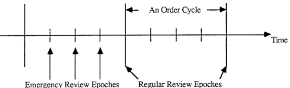
Figure 1. An order cycle with four periods.
the reviewing costs or how the coordination of orders for different items is accomplished. We simply assume that the length of review periods has already been determined by the organization and a regular order is placed after ( and only after ) every review. Such an operating policy, known as a replenishment cycle system, is in common use ( see, e.g., Silver and Peterson [17 ] ) . As we consider review periods that are long, we will rename them order cycles thereafter.
We assume that at a regular review epoch, an emergency order could be placed in addition to a regular order if justified by an urgent situation. In addition, since the order cycles are long, if an urgent situation should arise at any time between two regular review epochs, an emergency order can be placed immediately to have the inventory replenished and thus avoid any possible stockouts that might occur if replenishment is postponed until a regular review epoch. With the existing computer storage and updating capability, the number of applications in which the inventory position for each item is virtually known at any time increases significantly. To develop our model, we hypothesize that there are a number of periods ( to be somewhat consistent with the literature ) , which are of length 1 working day, within an order cycle. Regular orders are placed at regular review epochs while emergency orders could be placed at both regular review epochs and period review epochs ( called emergency review epochs, see Figure 1 ) . This kind of inventory control system is common in the import auto industry in Taiwan. For example, Hotai Motor Co. Ltd. mentioned above replenishes the inventory of auto parts by ship as well as by air. In the former case, it weekly orders thousands of auto parts ( there is an order-up-to level for each part ) from Toyota Motor Company in Japan. In the latter case, if the inventory level of a part ( usually an A item) falls below a warning point, it places an emergency order ( whose lead time is about one week ) . Notice that, in Chiang and Gutierrez [ 6 ] , a periodic system with long-order cycles is also considered. However, emergency long-orders as well as regular long-orders are placed only at regular review epochs due to the fact that inventory position of each item is not known at any time between two regular reviews. Also, Chiang and Gutierrez [ 6 ] considers only the case in which emergency orders have same variable costs ( as the regular orders ) but larger fixed order costs.
Although our model is closely related to the one in Moinzadeh and Nahmias [13 ] , there are important differences between these two models. From an operational point of view, both models allow the placement of emergency orders at any time. However, while Moinza-deh and Nahmias’ continuous review model places regular orders on continuous time, our model places regular orders only on periodic epochs ( due to the fact of coordinated ordering or purchasing from the same source ) . No model subsumes the other. They simply describe different operating systems used in practice. From a theoretical point of view, while
Moinza-deh and Nahmias evaluate an assumed policy, this research derives the form of the optimal policy and algorithms for computing it.
We analyze the problem within the framework of a stochastic dynamic program. We assume that the difference between the regular and emergency supply lead times is larger than one period ( for the case in which the difference between the two lead times is exactly one period, see Chiang [ 5 ] ) , and that a larger unit item cost is associated with the use of the emergency supply channel. It is possible that emergency orders have both fixed order costs and larger variable costs. This paper, however, treats only a special case; i.e., we assume that emergency fixed costs are negligible. We will develop a recursive formulation for the finite horizon problem, and derive conditions to verify the convergence of the regular and emergency ordering policies as the planning horizon is extended. Hence, the ordering rules to which these policies respectively converge are optimal for the infinite horizon model.
The optimal control policy derived is a natural extension of the optimal order-up-to- R ordering policy for the ordinary one-supply-mode model. As we shall see, the optimal operation parameters are obtained once a stopping condition is satisfied. Thus, the optimal control policy is easy to compute.
2. A DYNAMIC PROGRAMMING MODEL
Assume that there are two supply modes available: namely, a regular mode and an
emergency mode. The unit item costs for the regular and emergency supply modes are c1
and c0respectively, where c1õc0. Let m be the number of periods within an order cycle.
We assume that the difference between the regular and emergency supply lead times is smaller than m periods but larger than one period. For notational simplicity, we assume that the emergency and regular supply lead times are one and t periods respectively, where
3°t°m . Assume that all demand which is not filled immediately is backlogged. There
are inventory holding and shortage costs which are charged based on the net inventory ( i.e., inventory on hand minus backorder ) at the end of each period according to a loss function ,(r) . Let F( t ) be the probability distribution function for demand t during a period with mean m. Demand is assumed to be nonnegative and independently distributed in disjoint time intervals. Let aÛbåmax { a , b } .
Suppose the net inventory at the beginning of a period is x ; then the expected holding and shortage costs incurred in that period are given by
L ( x ) Å
*
`
0
,( x0t ) d F( t ) . ( 1 )
Other functional forms of L ( x ) are allowed; however, for our analysis we need L ( x ) to be a convex and differentiable function. Define Vi ,j( x , y ) as the expected discounted cost with
i order cycles and j periods remaining ( 0 ° j ° m 0 1 ) until the end of the planning
horizon, when the starting net inventory is x , inventory on order is y ( y ¢ 0 ) , and an optimal ordering policy is used at every review epoch. For simplicity of formulation, only the costs affected by the decision made at the current epoch are included in Vi ,j( x , y ) . As inventory on order is zero when there are less than m0t/1 periods remaining, Vi ,j( x ,
y ) simplifies to Vi ,j( x , 0 ) for jÅ0, 1, . . . , m0t. Then, Vi ,j( x , y ) satisfies the functional
Vi ,0( x , 0 )Å min x°r,z¢0 { c0r/c1z/aEtL ( r0t )/ aEtVi01,m01( r0t , z ) }0c0x , ( 2 ) Vi ,j( x , y ) Åmin x°r { c0r/aEtL ( r0t )/ aEtVi ,j01( r0 t , y ) }0c0x , j Å1, . . . , m01 and j xm0t/1, ( 3 ) Vi ,m0 t/1( x , y )Åmin x°r { c0r/aEtL ( y/r0t )/aEtVi ,m0 t( y/r0t , 0 ) }0c0x , ( 4 )
where V0,0( x , 0 ) å 0, a ( 0 õ a õ 1 ) is the discount factor, r is the inventory position
after a possible emergency order is placed at a review epoch, and z is the quantity ordered via the regular supply mode at a regular review epoch which becomes inventory on order thereafter. As we see, obtaining Vi ,0( x , 0 ) requires computations of the order of O ( imX3) , where X is the domain of the state x . Define
Ji( r ) Åmin z¢0 { Ji ,0( r , z ) } , ( 5 ) where Ji ,0( r , z )Åc1z/aEtVi01,m01( r0t , z ) . ( 6 ) Then ( 2 ) is expressed as Vi ,0( x , 0 )Å min x°r { c0r/aEtL ( r0t )/minz¢0 { Ji ,0( r , z ) } }0c0x Åmin x°r { c0r/aEtL ( r0t ) / Ji( r ) }0c0x . ( 7 ) Define Gi ,0( r )Åc0r/aEtL ( r0t ) / Ji( r ) , ( 8 ) Gi ,j( r , y )Åc0r/ aEtL ( r0t )/aEtVi ,j01( r0t , y ) , jÅ1, . . . , m 01 and jxm 0t/1, ( 9 ) Gi ,m0 t/1( r , y )Åc0r/aEtL ( y/r0t ) /aEtVi ,m0 t( y/r 0t , 0 ) . ( 10 )
[ Note that as there is no inventory on order after the regular order arrives, Gi ,j( r , y ) simplifies to Gi ,j( r , 0 ) for jÅ1, . . . , m0t.] Then ( 7 ) , ( 3 ) , and ( 4 ) can be rewritten as
Vi ,0( x , 0 )Åmin x°r { Gi ,0( r ) } 0c0x , ( 11 ) Vi ,j( x , y )Åmin x°r { Gi ,j( r , y ) }0c0x , jÅ1, . . . , m 01. ( 12 )
LEMMA 1: Vi ,j( x , y ) for each ( i , j ) is a convex function. PROOF: See the Appendix.
Let ri ,jbe the ( smallest ) value minimizing Gi ,jas given in expressions ( 8 ) – ( 10 ) . For j Åm0t/1, . . . , m01, ri ,j[ written as ri ,j( y ) if there is ambiguity ] is a function of y , i.e., the optimal emergency order-up-to level is a function of the inventory on order. Also, let zi( r ) be the ( smallest ) value of nonnegative z that minimizes Ji ,0( r , z ) for a given r , i.e., the optimal regular order quantity at a regular review epoch is a function of the inventory position after a possible emergency order is placed at that epoch. Then the optimal policy at a regular review epoch is ( i ) order up to ri ,0at unit cost c0if x õri ,0and ( ii ) order the amount zi( xÛ ri ,0) at unit cost c1; and the optimal policy at an emergency review epoch
is ( i ) order up to ri ,jat unit cost c0if xõri ,jand ( ii ) do not order if x ¢ri ,j.
3. PROPERTIES OF THE MODEL
In this section, we present important properties for the model developed in Section 2. We first introduce some observations that will be used extensively to establish the results of this section. Denote by Df the first derivative of the function f and by Dif the first derivative of the function f with respect to its i th variable. It follows from ( 11 ) , ( 12 ) , and the definition of ri ,jthat D1Vi ,j( x , y ) Å 0c0for x°ri ,j, and D1Vi ,j( x , y ) ¢ 0c0for all x .
Also, as we see from ( 12 ) , Vi ,j( x , y ) , for jÅm 0t/1, . . . , m0 1, can be written as Vi ,j( x , y )ÅGi ,j( x Ûri ,j( y ) , y )0c0x , jÅ m0t/1, . . . , m 01. ( 13 )
Consequently, we have that for x°ri ,j( y ) , D2Vi ,j( x , y )ÅD2Gi ,j( ri ,j( y ) , y )/D1Gi ,j( ri ,j( y ) , y )rDri ,j( y )ÅD2Gi ,j( ri ,j( y ) , y ) since D1Gi ,j( ri ,j( y ) , y )Å0 [ ri ,j( y ) minimizes Gi ,j( r , y ) by definition ] . For x¢ ri ,j( y ) , D2Vi ,j( x , y ) ÅD2Gi ,j( x , y ) .
We show in Theorem 1 that the emergency order-up-to levels within an order cycle,
which can be separated into two groups ( if tõ m ) according to whether or not there is
inventory on order, are nondecreasing in each group.
THEOREM 1: ri ,m0 t ¢ ri ,m0 t01 ¢ rrr ¢ ri ,1 and ri ,m01( y ) ¢ ri ,m02( y ) ¢ rrr
¢ri ,m0 t/1( y ) .
PROOF: See the Appendix.
We next show that the emergency order-up-to level ri ,m0 t/1 is a linearly decreasing
function of inventory on order y . Let D denote a positive real number.
THEOREM 2: ri ,m0 t/1( y ) is decreasing in y . In addition, ri ,m0 t/1( y )Åri ,m0 t/1( 0 )0y .
PROOF: See the Appendix.
Theorem 2 confirms our intuition that we shall be less willing to use the emergency mode at the current review epoch if the inventory on order we will receive at the next epoch is larger. Next, we show that emergency order-up-to levels ri ,j( y), jÅm 0t/2, m0t/
3, . . . , m01, are nonincreasing in inventory on order, and that if they decrease as inventory on order increases, they decrease by an amount that is less than or equal to the amount by which inventory on order increases. We first state an important preliminary lemma.
LEMMA 2: The mixed second derivative of Vi ,m0 t/1( x , y ) is nonnegative, i.e.,
D1Vi ,m0 t/1( x , y )°D1Vi ,m0 t/1( x , y/D ) [ or D2Vi ,m0 t/1( x0D, y )°D2Vi ,m0 t/1( x , y ) ] .
In addition, D1Vi ,m0 t/1( x 0 D, y / D ) Å D1Vi ,m0 t/1( x , y ) Å D2Vi ,m0 t/1( x , y ) Å
D2Vi ,m0 t/1( x0D, y/D ) .
PROOF: See the Appendix.
THEOREM 3: ri ,m0 t/2( y ) is nonincreasing in y , i.e., ri ,m0 t/2( y ) ¢ ri ,m0 t/2( y / D ) .
Moreover, ri ,m0 t/2( y ) 0ri ,m0 t/2( y/D ) °D.
PROOF: See the Appendix.
LEMMA 3: The mixed second derivative of Vi ,m0 t/2( x , y ) is nonnegative, i.e.,
D1Vi ,m0 t/2( x , y )°D1Vi ,m0 t/2( x , y/D ) [ or D2Vi ,m0 t/2( x0D, y )°D2Vi ,m0 t/2( x , y ) ] .
In addition, D1Vi ,m0 t/2( x 0 D, y / D ) ° D1Vi ,m0 t/2( x , y ) and D2Vi ,m0 t/2( x , y ) °
D2Vi ,m0 t/2( x0D, y/D ) .
PROOF: See the Appendix.
COROLLARY: For jÅm 0t/3, . . . , m01, ri ,j( y )¢ri ,j( y/ D )¢ ri ,j( y )0D. Moreover, D1Vi ,j( x0 D, y/ D ) °D1Vi ,j( x , y ) °D1Vi ,j( x , y/D ) and D2Vi ,j( x0 D, y )° D2Vi ,j( x , y ) °D2Vi ,j( x0 D, y/D ) .
Next, we show that the quantity we order via the regular supply mode at a regular review epoch is nonincreasing in the starting net inventory ( or the inventory position after a possible emergency order is placed at that epoch ) . This conforms the intuition that we shall order less if we start with more inventory. Moreover, if the quantity ordered via the regular mode decreases as the starting net inventory ( or the inventory position after a possible emergency order ) increases, it decreases by an amount that is less than or equal to the amount by which the starting net inventory increases.
THEOREM 4: zi( x Ûri ,0) is nonincreasing in x , i.e., zi( r ) ° zi( r 0D ) . In addition, zi( r0D ) 0D° zi( r ) .
PROOF: See the Appendix.
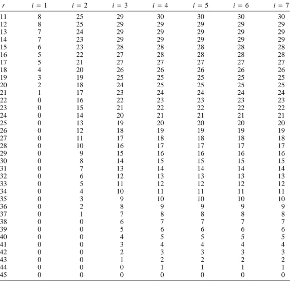
To illustrate, consider the example: mÅ10 periods, t Å6 periods, c1Å$10, c0Å$15,
mÅ2 ( with Poisson demand ) , ,( x )Å .01 x for xú 0 and,( x ) Å 020 x for xõ 0 ( this choice of the loss function implies that the holding and shortage costs are $.01 and $20 per unit respectively ) , and a Å 0.999. The resulting optimal policy zi( r ) and ri ,j( y ) is
Table 1. Regular order quantity zi(r) as a function of r (i.e., inventory position after a possible
emergency order is placed at a regular review epoch)a
. r iÅ 1 iÅ 2 iÅ 3 iÅ 4 iÅ 5 iÅ 6 iÅ 7 11 8 25 29 30 30 30 30 12 8 25 29 29 29 29 29 13 7 24 29 29 29 29 29 14 7 23 29 29 29 29 29 15 6 23 28 28 28 28 28 16 5 22 27 28 28 28 28 17 5 21 27 27 27 27 27 18 4 20 26 26 26 26 26 19 3 19 25 25 25 25 25 20 2 18 24 25 25 25 25 21 1 17 23 24 24 24 24 22 0 16 22 23 23 23 23 23 0 15 21 22 22 22 22 24 0 14 20 21 21 21 21 25 0 13 19 20 20 20 20 26 0 12 18 19 19 19 19 27 0 11 17 18 18 18 18 28 0 10 16 17 17 17 17 29 0 9 15 16 16 16 16 30 0 8 14 15 15 15 15 31 0 7 13 14 14 14 14 32 0 6 12 13 13 13 13 33 0 5 11 12 12 12 12 34 0 4 10 11 11 11 11 35 0 3 9 10 10 10 10 36 0 2 8 9 9 9 9 37 0 1 7 8 8 8 8 38 0 0 6 7 7 7 7 39 0 0 5 6 6 6 6 40 0 0 4 5 5 5 5 41 0 0 3 4 4 4 4 42 0 0 2 3 3 3 3 43 0 0 1 2 2 2 2 44 0 0 0 1 1 1 1 45 0 0 0 0 0 0 0 aData: m Å 10, c
1 Å $10, c0 Å $15, ,(x) Å .01x for x ú 0 and ,(x) Å 020x for x õ 0, m Å 2
(Poisson demand), aÅ 0.999, and t Å 6.
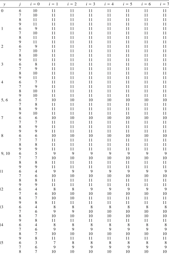
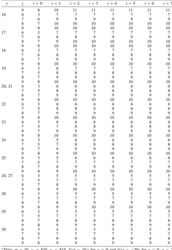
reported in Tables 1 and 2. As we can observe from these tables, all policy parameters seem to converge after a few order cycles. For example, from Table 1 we see that zi( 20 ) Å2, 18, 24, 25, 25, 25, 25 for i Å1, . . . , 7. From Table 2, we also see that ri ,6( 15 )Å3, 7, 8, 8, 8, 8, 8, 8 for iÅ0, 1, . . . , 7. Similar convergence properties can be observed for all other parameter values in Tables 1 and 2. A natural question at this point is whether or not this observed convergence property holds in general. We show in the final part of this section that this is indeed true if certain conditions are satisfied.
Let Ri be the minimum value of r for which zi( r ) Å0. We assume that Ri ú ri ,0, i.e., zi( ri ,0) ú 0; otherwise, the regular supply mode is never used. It follows by Theorem 4 that, for all r°Ri, r /zi( r )° Ri /zi( Ri) ÅRi. This implies that Ri is the maximum
Table 2. Emergency order-up-to levels ri,j, jÅ 6, . . . , 9, as a function of inventory on order y a . y j iÅ 0 iÅ 1 iÅ 2 iÅ 3 iÅ 4 iÅ 5 iÅ 6 iÅ 7 0 6 10 11 11 11 11 11 11 11 7 10 11 11 11 11 11 11 11 8 11 11 11 11 11 11 11 11 9 11 11 11 11 11 11 11 11 1 6 9 11 11 11 11 11 11 11 7 10 11 11 11 11 11 11 11 8 11 11 11 11 11 11 11 11 9 11 11 11 11 11 11 11 11 2 6 9 11 11 11 11 11 11 11 7 10 11 11 11 11 11 11 11 8 10 11 11 11 11 11 11 11 9 11 11 11 11 11 11 11 11 3 6 8 11 11 11 11 11 11 11 7 9 11 11 11 11 11 11 11 8 10 11 11 11 11 11 11 11 9 11 11 11 11 11 11 11 11 4 6 7 11 11 11 11 11 11 11 7 9 11 11 11 11 11 11 11 8 10 11 11 11 11 11 11 11 9 10 11 11 11 11 11 11 11 5, 6 6 7 10 10 10 10 10 10 10 7 8 11 11 11 11 11 11 11 8 9 11 11 11 11 11 11 11 9 10 11 11 11 11 11 11 11 7 6 6 10 10 10 10 10 10 10 7 7 11 11 11 11 11 11 11 8 9 11 11 11 11 11 11 11 9 9 11 11 11 11 11 11 11 8 6 6 10 10 10 10 10 10 10 7 7 11 11 11 11 11 11 11 8 8 11 11 11 11 11 11 11 9 9 11 11 11 11 11 11 11 9, 10 6 5 9 9 9 9 9 9 9 7 7 10 10 10 10 10 10 10 8 8 11 11 11 11 11 11 11 9 9 11 11 11 11 11 11 11 11 6 4 9 9 9 9 9 9 9 7 6 10 10 10 10 10 10 10 8 8 11 11 11 11 11 11 11 9 9 11 11 11 11 11 11 11 12 6 4 8 8 9 9 9 9 9 7 6 10 10 10 10 10 10 10 8 7 10 10 11 11 11 11 11 9 8 11 11 11 11 11 11 11 13 6 4 8 8 8 8 8 8 8 7 6 9 9 10 10 10 10 10 8 7 10 10 10 10 10 10 10 9 8 11 11 11 11 11 11 11 14 6 4 8 8 8 8 8 8 8 7 6 9 9 9 9 9 9 9 8 7 10 10 10 10 10 10 10 9 8 11 11 11 11 11 11 11 15 6 3 7 8 8 8 8 8 8 7 6 9 9 9 9 9 9 9 8 7 10 10 10 10 10 10 10
Table 2. Continued y j iÅ 0 iÅ 1 iÅ 2 iÅ 3 iÅ 4 iÅ 5 iÅ 6 iÅ 7 9 8 10 11 11 11 11 11 11 16 6 3 7 7 7 7 7 7 7 7 6 9 9 9 9 9 9 9 8 7 10 10 10 10 10 10 10 9 8 10 10 10 10 10 10 10 17 6 3 7 7 7 7 7 7 7 7 6 8 8 9 9 9 9 9 8 7 9 10 10 10 10 10 10 9 8 10 10 10 10 10 10 10 18 6 3 7 7 7 7 7 7 7 7 6 8 8 8 8 8 8 8 8 7 9 9 9 9 9 9 9 9 8 10 10 10 10 10 10 10 19 6 3 6 7 7 7 7 7 7 7 5 8 8 8 8 8 8 8 8 7 9 9 9 9 9 9 9 9 8 10 10 10 10 10 10 10 20, 21 6 3 6 6 6 6 6 6 6 7 5 8 8 8 8 8 8 8 8 7 9 9 9 9 9 9 9 9 8 10 10 10 10 10 10 10 22 6 3 6 6 6 6 6 6 6 7 5 8 8 8 8 8 8 8 8 7 9 9 9 9 9 9 9 9 8 10 10 10 10 10 10 10 23 6 3 6 6 6 6 6 6 6 7 5 7 8 8 8 8 8 8 8 7 9 9 9 9 9 9 9 9 8 10 10 10 10 10 10 10 24 6 3 5 6 6 6 6 6 6 7 5 7 8 8 8 8 8 8 8 7 9 9 9 9 9 9 9 9 8 9 10 10 10 10 10 10 25 6 3 5 6 6 6 6 6 6 7 5 7 7 7 7 7 7 7 8 7 8 9 9 9 9 9 9 9 8 9 10 10 10 10 10 10 26, 27 6 3 5 5 5 5 5 5 5 7 5 7 7 7 7 7 7 7 8 7 8 9 9 9 9 9 9 9 8 9 10 10 10 10 10 10 28 6 3 5 5 5 5 5 5 5 7 5 7 7 7 7 7 7 7 8 7 8 8 9 9 9 9 9 9 8 9 9 10 10 10 10 10 29 6 3 5 5 5 5 5 5 5 7 5 7 7 7 7 7 7 7 8 7 8 8 8 8 8 8 8 9 8 9 9 9 9 9 9 9 30 6 3 4 5 5 5 5 5 5 7 5 7 7 7 7 7 7 7 8 7 8 8 8 8 8 8 8 9 8 9 9 9 9 9 9 9 aData: m Å 10, c
1 Å $10, c0 Å $15, ,(x) Å .01x for x ú 0 and ,(x) Å 020x for x õ 0, m Å 2
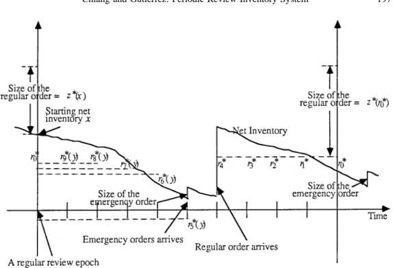
Figure 2. A realization of the inventory process for the periodic system in which the emergency and regular supply lead times are one and six periods, respectively.
possible order-up-to level ( or inventory position ) with i order cycles remaining if a regular order is placed at that epoch. Let Zi be the maximum possible regular order quantity with
i cycles remaining. Then, Zi Åzi( ri ,0) by Theorem 4 and for all y ° Zi, y /ri01,m01( y )
°Zi /ri01,m01(Zi) by the corollary. We show in Theorem 5 that if, for a regular review epoch, the two consecutive maximum order-up-to levels are equal to each other, i.e., Ri Å Ri01, and greater than every intermediate emergency order-up-to level ( plus, if any, a regular
order quantity ) , i.e., Ri ¢ri01,m0 tand Ri ¢ri01,m01(Zi) /Zi, and the first derivatives for these two consecutive cost functions are equal, i.e., D1Vi ,0( x , 0 )ÅD1Vi01,0( x , 0 ) for x°
Ri, then the sequences { rn ,0} , { rn ,j} for j Å1, . . . , m0t, { rn ,j( y ) } for jÅm0t/1, . . . , m01, and { zn( r ) , r ¢rn ,0} converge respectively to r *0 Åri ,0, r *j Åri01, jfor jÅ
1, . . . , m0t, r *j ( y )Åri01, j( y ) for jÅm0 t/ 1, . . . , m0 1, and z *( r )Åzi( r ) for r¢r *0. As a result, r *j for jÅ0, 1, . . . , m0t, r *j ( y ) for jÅm0t/1, . . . , m 01, and z *( r ) for r ¢ r *0, are, respectively, the optimal emergency order-up-to levels and
regular order quantities for the infinite horizon model ( see Figure 2 for an example of a realization of the inventory process over an infinite horizon ) .
THEOREM 5: If there exists some i such that ( a ) Ri ÅRi01( Ri ú ri ,0) ,
( b ) Ri ¢ri01,m0 t, Ri ¢ ri01,m01(Zi)/ Zi, ( c ) D1Vi ,0( x , 0 )ÅD1Vi01,0( x , 0 ) for x °Ri, then the following convergence properties hold
( i ) rn ,jÅri01, j, jÅ1, . . . , m0t ( if tõm ) , n¢i , rn ,j( y )Åri01, j( y ) for y°Ri0ri01, j( y ) , jÅm0t/1, . . . , m01, n¢i ; ( 14 ) ( ii ) zn/1( r ) Åzi( r ) for r° Ri, n¢i , rn/1,0Åri ,0and Rn/1ÅRi ( thus Zn/1ÅZi) , n¢i . ( 15 )
PROOF: See the Appendix.
Theorem 5 states that if conditions ( a ) , ( b ) , and ( c ) are satisfied, convergence of all operation parameters has been obtained and thus computation can be stopped. Referring to the example discussed above, as we see from Tables 1 and 2, convergence is obtained after just five order cycles ( as a note, R5 Å 45, r *0 Å r5,0 Å11, and Z5 Å 30 ) . We note that
condition ( a ) can be easily satisfied, and condition ( b ) is expected to hold. The latter is because Ri( as explained before Theorem 5 ) should be large enough to cover demand over an order cycle plus the regular supply lead time as it will take m/t periods for the next
regular order to arrive, and similarly, ri01,m01(Zi) /Zi, for example, should meet demand over a time interval of m/t01 periods ( which is shorter by one period ) .
4. COMPUTATIONAL RESULTS
In this section, we test a set of problems to investigate the speed of convergence of operation parameters ri ,j, jÅ0, 1, . . . , m0 t, ri ,j( y ) , jÅm 0t/ 1, . . . , m01, and zi( r ) . To this end, we define ,( x )Åhx for xú0,,( 0 )Å0, and,( x ) Å 0px for xõ0 ( i.e., the holding and shortage costs are charged at the rates of h and p , respectively ) . Also, we use the following end-of-horizon condition ( to speed the computation ) : V0,0( x , 0 ) å
0c0x for x õ0, V0,0( 0, 0 )å0, and V0,0( x , 0 )å 0c1x for xú0.
For the purposes of this experiment, we say that the first derivatives of two consecutive cost functions ( at regular review epoches ) could be regarded as equal when
Max x°Ri
ÉD1Vi ,0( x , 0 )0D1Vi01,0( x , 0 )É °1, ( 16 )
where 1 is set to 0.02 for all problems we solve ( using FORTRAN on an IBM-3081 computer with a VMS operating system) .
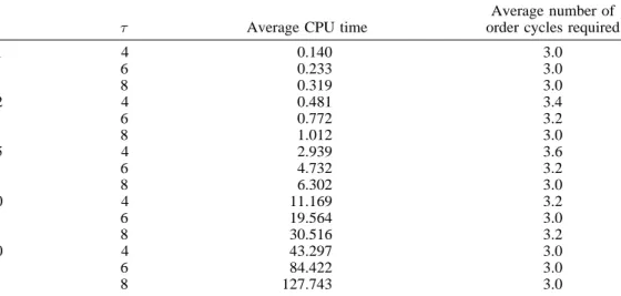
Table 3. CPU time (s) and number of order cycles required for the convergence of operation parametersa
.
Average number of
m t Average CPU time order cycles required
1 4 0.140 3.0 6 0.233 3.0 8 0.319 3.0 2 4 0.481 3.4 6 0.772 3.2 8 1.012 3.0 5 4 2.939 3.6 6 4.732 3.2 8 6.302 3.0 10 4 11.169 3.2 6 19.564 3.0 8 30.516 3.2 20 4 43.297 3.0 6 84.422 3.0 8 127.743 3.0 aCommon data: mÅ 10, c
1Å $10, h Å $0.01, a Å 0.999. For each combination of m and t, five
problems with different values of c0and p are solved, i.e., (c0, p)Å (15, 20), (15, 40), (15, 60), (20,
40), or (20, 60).
As shown in Table 3, 15 combinations of different values of m and t are formed, and, for each combination, there are five problems varying on values of c0and p . Thus, there
are a total of 75 problems. For each problem, the CPU time ( in seconds ) and number of order cycles required ( for the convergence to occur ) are recorded. The average CPU time and the average number of order cycles required for each combination are reported in Table 3. As we see, the average number of order cycles required is between 3.0 and 3.4. In fact, the maximum and minimum number of order cycles required across all problems are 5 and 3, respectively. However, the average CPU time required increases ( approximately ) linearly in t and ( approximately ) quadratically in m. The latter implies that if mean demand ( per period ) is very large, we may need to rescale the data to accommodate the problem so that it can be solved within reasonable time.
5. CONCLUSION
In this paper, we study a periodic review inventory system in which regular orders are placed periodically while emergency orders can be placed continuously. Assuming that the difference between the regular and emergency channel lead times is greater than one period but less than the order-cycle length, we develop a dynamic programming model and derive a stopping rule to end the computation and obtain optimal operation parameters. Computa-tional results are included that support the contention that easily implemented policies can be computed with reasonable effort.
Extension of the analysis to the case in which the two channel lead times differ by more than an order cycle appears to be difficult. The problem lies in the need of keeping track of every amount of inventory on order, which would increase the state space from two dimensions to multiple dimensions. This is left for future research.
APPENDIX
PROOF OF LEMMA 1: V0,0( x , 0 ) is convex. Assuming that V0, j01( x , 0 ) , j°m0t, is convex, we show that
V0, j( x , 0 ) is convex. It follows from ( 9 ) that G0, j( r , 0 ) is a convex function. Hence, V0, j( x , 0 ) is convex by Proposition B-4 of Heyman and Sobel [12 ] . Since V0,m0 t( x , 0 ) is convex, G0,m0 t/1( r , y ) is jointly convex in r
and y . Thus, V0,m0 t/1( x , y ) is jointly convex in x and y by Proposition B-4 of Heyman and Sobel [12 ] , and so
are V0, j( x , y ) , jÅm0t/2, . . . , m01. Hence, J1( r ) is convex in r and V1,0( x , 0 ) is convex in x by their Proposition B-4. Convexity is established by induction for Vi ,j( x , y ) , i¢1. h
PROOF OF THEOREM 1: We first show that ri ,m0 t¢ri ,m0 t01¢ rrr ¢ri ,1. We show that ri ,2¢ri ,1. The
remaining inequalities can be established similarly. To show ri ,2¢ri ,1, we show that D1Gi ,2( r , 0 )õ0 for rõ
ri ,1. It follows from ( 9 ) and definition of ri ,jthat D1Gi ,1( r , 0 )Åc0/aEtDL ( r0t )/aEtD1Vi ,0( r0t , 0 )õ0
for rõri ,1. Also, from the observations mentioned in the text, D1Gi ,2( r , 0 )Åc0/aEtDL ( r0t )/aEtD1Vi ,1( r
0t , 0 )Åc0/aEtDL ( r0t )0ac0for rõri ,1. Hence, D1Gi ,2( r , 0 )õ 0a[ c0/EtD1Vi ,0( r0t , 0 ) ]°0, for
rõri ,1.
We next show that ri ,m01( y )¢ri ,m02( y )¢ rrr ¢ri ,m0 t/1( y ) . We show that ri ,m0 t/2( y )¢ri ,m0 t/1( y ) is true.
The remaining inequalities can be established similarly. To show ri ,m0 t/2( y ) ¢ ri ,m0 t/1( y ) , we show that
D1Gi ,m0 t/2( r , y )õ0 for rõri ,m0 t/1( y ) . It follows from ( 9 ) and ( 10 ) that
D1Gi ,m0 t/1( r , y )Åc0/aEtDL ( y/r0t )/aEtD1Vi ,m0 t( y/r0t , 0 ) , ( 17 )
D1Gi ,m0 t/2( r , y )Åc0/aEtDL ( r0t )/aEtD1Vi ,m0 t/1( r0t , y ) . ( 18 )
As ri ,m0 t/1( y ) is the smallest value minimizing Gi ,m0 t/1( r , y ) , D1Gi ,m0 t/1( r , y )õ0 for rõri ,m0 t/1( y ) , i.e.,
aEtDL ( y/r0t )õ 0c00aEtD1Vi ,m0 t( y/r0t , 0 ) for rõri ,m0 t/1( y ) . However, D1Gi ,m0 t/2( r , y )Åc0/
aEtDL ( r0t )0ac0for rõri ,m0 t/1( y ) ( by the observations in the text ) . It follows then from the convexity of
L (r) and y¢0 that D1Gi ,m0 t/2( r , y )°c0/aEtDL ( y/r0t )0ac0õ 0a[ c0/EtD1Vi ,m0 t( y/r0t , 0 ) ]
°0 for rõri ,m0 t/1( y ) . h
PROOF OF THEOREM 2: As we see from ( 17 ) , ri ,m0 t/1( y ) minimizing Gi ,m0 t/1( r , y ) will decrease as y
increases. In fact, a change of variables in ( 17 ) ( i.e., y/r is denoted by a single variable ) shows that ri ,m0 t/1( y )
Åri ,m0 t/1( 0 )0y and ri ,m0 t/1( y/D )Åri ,m0 t/1( y )0D. h
PROOF OF LEMMA 2: ri ,m0 t/1( y/D )Åri ,m0 t/1( y )0Dõri ,m0 t/1( y ) by Theorem 2. Hence, ( i ) for x°
ri ,m0 t/1( y/D ) , D1Vi ,m0 t/1( x , y )ÅD1Vi ,m0 t/1( x , y/D )Å 0c0; ( ii ) for x√( ri ,m0 t/1( y/D ) , ri ,m0 t/1( y ) ) ,
D1Vi ,m0 t/1( x , y )Å 0c0°D1Vi ,m0 t/1( x , y/D ) ; and ( iii ) for x¢ri ,m0 t/1( y ) ,
D1Vi ,m0 t/1( x , y )ÅaEtDL ( y/x0t )/aEtD1Vi ,m0 t( y/x0t , 0 )
°aEtDL ( y/D/x0t )/aEtD1Vi ,m0 t( y/D/x0t , 0 )
Å D1Vi ,m0 t/1( x , y/D ) ,
due to ( 13 ) , ( 17 ) , and Lemma 1. We have shown that the mixed second derivative of Vi ,m0 t/1( x , y ) is nonnegative.
In addition, it follows from ( 17 ) and the observations mentioned in the text that for x°ri ,m0 t/1( y ) or x0D°
ri ,m0 t/1( y/D ) ,
D1Vi ,m0 t/1( x , y )Å D1Vi ,m0 t/1( x0D, y/D )Å 0c0
ÅaEtDL ( y/ri ,m0 t/1( y )0t )/aEtD1Vi ,m0 t( y/ri ,m0 t/1( y )0t , 0 ) ,
D2Vi ,m0 t/1( x , y )Å D2Vi ,m0 t/1( x0D, y/D )
ÅaEtDL ( y/D/ri ,m0 t/1( y/D )0t )/aEtD1Vi ,m0 t( y/D/ri ,m0 t/1( y/D )0t , 0 ) .
As ri ,m0 t/1( y/D )/DÅri ,m0 t/1( y ) , the above two expressions are equal. Also, for xúri ,m0 t/1( y ) or x0
Dúri ,m0 t/1( y/D ) ,
Å D2Vi ,m0 t/1( x , y ) , D1Vi ,m0 t/1( x0D, y/D )Å D2Vi ,m0 t/1( x0D, y/D ) ÅaEtDL ( y/D/x0D0t )/aEtD1Vi ,m0 t( y/D/x0D0t , 0 ) ÅaEtDL ( y/x0t )/aEtD1Vi ,m0 t( y/x0t , 0 ) . As a result, D1Vi ,m0 t/1( x , y )ÅD2Vi ,m0 t/1( x , y )ÅD1Vi ,m0 t/1( x0D, y/D )ÅD2Vi ,m0 t/1( x0D, y/D ) . h
PROOF OF THEOREM 3: It follows from Lemma 2 that
D1Gi ,m0 t/2( r , y )Å c0/aEtDL ( r0t )/aEtD1Vi ,m0 t/1( r0t , y )
° c0/aEtDL ( r0t )/aEtD1Vi ,m0 t/1( r0t , y/D )ÅD1Gi ,m0 t/2( r , y/D ) .
This implies that ri ,m0 t/2( y )¢ri ,m0 t/2( y/D ) . Furthermore, as D1Vi ,m0 t/1( x0D, y/D )ÅD1Vi ,m0 t/1( x , y )
by Lemma 2,
D1Gi ,m0 t/2( r , y )Åc0/aEtDL ( r0t )/aEtD1Vi ,m0 t/1( r0D0t , y/D )¢c0/aEtDL ( r0D0t )
/aEtD1Vi ,m0 t/1( r0D0t , y/D )ÅD1Gi ,m0 t/2( r0D, y/D ) .
As D1Gi ,m0 t/2( r , y )õ0 for rõri ,m0 t/2( y ) , it follows that D1Gi ,m0 t/2( r0D, y/D )õ0 for rõri ,m0 t/2( y )
or r0Dõri ,m0 t/2( y )0D. This implies that ri ,m0 t/2( y/D )¢ri ,m0 t/2( y )0D. h
PROOF OF LEMMA 3: For the nonnegativity of the mixed second derivative of Vi ,m0 t/2( x , y ) , the proof is
similar to that of Lemma 2. We show that the other part of this lemma is true. By Theorem 3, ri ,m0 t/2( y/D )
/D¢ri ,m0 t/2( y ) . It follows from ( 18 ) and Lemma 2 ( and observations mentioned in the text ) that ( i ) for x
°ri ,m0 t/2( y ) [ and thus x0D°ri ,m0 t/2( y/D ) ] , D1Vi ,m0 t/2( x , y )Å 0c0ÅD1Vi ,m0 t/2( x0D, y/D ) and
D2Vi ,m0 t/2( x , y )ÅaEtD2Vi ,m0 t/1( ri ,m0 t/2( y )0t , y ) ÅaEtD2Vi ,m0 t/1( ri ,m0 t/2( y )0D0t , y/D )°aEtD2Vi ,m0 t/1( ri ,m0 t/2( y/D )0t , y/D ) ÅD2Vi ,m0 t/2( x0D, y/D ) ; ( ii ) for x¢ri ,m0 t/2( y/D )/D, D1Vi ,m0 t/2( x , y )ÅaEtDL ( x0t )/aEtD1Vi ,m0 t/1( x0t , y ) ÅaEtDL ( x0t )/aEtD1Vi ,m0 t/1( x0D0t , y/D ) ¢aEtDL ( x0D0t )/aEtD1Vi ,m0 t/1( x0D0t , y/D )ÅD1Vi ,m0 t/2( x0D, y/D ) and D2Vi ,m0 t/2( x , y )ÅaEtD2Vi ,m0 t/1( x0t , y ) ÅaEtD2Vi ,m0 t/1( x0D0t , y/D ) Å D2Vi ,m0 t/2( x0D, y/D ) ;
( iii ) finally, for x√( ri ,m0 t/2( y ) , ri ,m0 t/2( y/D )/D ) , D1Vi ,m0 t/2( x , y )¢ 0c0ÅD1Vi ,m0 t/2( x0D, y/D ) ,
and
D2Vi ,m0 t/2( x , y )ÅaEtD2Vi ,m0 t/1( x0t , y )ÅaEtD2Vi ,m0 t/1( x0D0t , y/D )
In summary, we have shown that D1Vi ,m0 t/2( x , y ) ¢D1Vi ,m0 t/2( x0 D, y/ D ) and D2Vi ,m0 t/2( x , y )°
D2Vi ,m0 t/2( x0D, y/D ) . h
PROOF OF THEOREM 4: It follows from Corollary and ( 6 ) that
D2Ji ,0( r0D, z )Åc1/aEtD2Vi01,m01( r0D0t , z )°c1/aEtD2Vi01,m01( r0t , z )ÅD2Ji ,0( r , z ) .
This implies that zi( r )°zi( r0D ) . Moreover, by the corollary
D2Ji ,0( r , z )Åc1/aEtD2Vi01,m01( r0t , z )°c1/aEtD2Vi01,m01( r0D0t , z/D )
ÅD2Ji ,0( r0D, z/D ) .
Since D2Ji ,0( r , z )¢0 for z¢zi( r ) , D2Ji ,0( r0D, z/D )¢0 for z¢zi( r ) or equivalently z/D¢zi( r )
/D. This implies that zi( r0D )°zi( r )/D. h
PROOF OF THEOREM 5: We divide the proof in three parts. Parts 1 and 2 show that ( 14 ) and ( 15 ) , respectively, hold for nÅi , and Part 3 establishes that D1Vi/1,0( x , 0 )ÅD1Vi ,0( x , 0 ) for x°Ri/1ÅRi. Thus,
the argument can be repeated and ( 14 ) and ( 15 ) hold for all n¢i .
Part 1. ( If tÅm , the proof starts in the next paragraph.) It follows from ( 9 ) that
D1Gi01,1( r , 0 )Åc0/aEtDL ( r0t )/aEtD1Vi01,0( r0t , 0 ) ,
D1Gi ,1( r , 0 )Åc0/aEtDL ( r0t )/aEtD1Vi ,0( r0t , 0 ) .
If D1Vi ,0( x , 0 )ÅD1Vi01,0( x , 0 ) for x°Ri, then D1Gi ,1( r , 0 )ÅD1Gi01,1( r , 0 ) for x°Ri. As Ri¢ri01,m0 t, Ri
¢ri01,1( by Theorem 1 ) . Since ri01,1minimizes Gi01,1( r , 0 ) , it follows that it also minimizes Gi ,1( r , 0 ) , i.e., ri ,1
Åri01,1. In addition, for xúri01,1, D1Vi01,1( x , 0 )ÅaEtDL ( x0t )/aEtD1Vi01,0( x0t , 0 ) and D1Vi ,1( x , 0 )Å
aEtDL ( x0t )/aEtD1Vi ,0( x0t , 0 ) . Hence, D1Vi ,1( x , 0 )ÅD1Vi01,1( x , 0 ) for x√( ri01,1, Ri] . Also, D1Vi ,1( x ,
0 )ÅD1Vi01,1( x , 0 )Å 0c0for x°ri01,1. As a result, D1Vi ,1( x , 0 )ÅD1Vi01,1( x , 0 ) for x°Ri. Similarly, we
can show that ri ,jÅri01, jfor jÅ2, . . . , m0t, and
D1Vi ,j( x , 0 )ÅD1Vi01, j( x , 0 ) , jÅ2, . . . , m0t, for x°Ri. ( 19 )
In addition, if Ri ¢ ri01,m01(Zi)/Zi, Ri ¢ri01,m0 t/1(Zi)/Zi Åri01,m0 t/1( 0 ) ( by Theorems 1 and 2 ) . By
using the same reasoning ( for showing ri ,1Åri01,1) , it follows from ( 17 ) and ( 19 ) that ri ,m0 t/1( 0 )Åri01,m0 t/1( 0 ) ,
and thus ri ,m0 t/1( y )Åri01,m0 t/1( y ) . Moreover, as D1Vi ,m0 t( x , 0 )ÅD1Vi01,m0 t( x , 0 ) for x°Ri, it can be seen
from ( 4 ) that
D1Vi ,m0 t/1( x , y )ÅD1Vi01,m0 t/1( x , y ) for x°Ri0y , ( 20 )
D2Vi ,m0 t/1( x , y )ÅD2Vi01,m0 t/1( x , y ) for y°Ri0x . ( 21 )
Likewise, we can show from ( 20 ) , ( 21 ) , ( 3 ) , and ( 9 ) that, for all y such that y/ ri01, j( y ) ° Ri, ri ,j( y )Å
ri01, j( y ) , jÅm0t/2, . . . , m01, and
D1Vi ,j( x , y )ÅD1Vi01, j( x , y ) for x°Ri 0y , jÅm0t/2, . . . , m01, ( 22 )
D2Vi ,j( x , y )ÅD2Vi01, j( x , y ) for y°Ri 0x , jÅm0t/2, . . . , m01. ( 23 )
Part 2. From ( 6 ) , D2Ji ,0( r , z )Åc1/aEtD2Vi01,m01( r0t , z ) and D2Ji/1,0( r , z )Åc1/aEtD2Vi ,m01( r0t ,
z ) . Hence, It follows from ( 23 ) that D2Ji/1,0( r , z )ÅD2Ji ,0( r , z ) for all z°Ri 0r . Also, for r°Ri, zi( r )°
Ri0r ( by Theorem 4 ) . As zi( r ) , r°Ri, minimizes Ji ,0( r , z ) , it follows that it also minimizes Ji/1,0( r , z ) , i.e.,
Since Riis the minimum value of r for which zi( r )Å0, it follows from ( 24 ) that Ri is also the minimum value
of r for which zi/1( r )Å0, i.e., Ri/1ÅRi.
Next, we show that ri/1,0Åri ,0( as a result, Zi/1ÅZi) . From ( 5 ) , Ji( r )ÅJi ,0( r , zi( r ) )Åc1zi( r )/aEtVi01,m01( r
0t , zi( r ) ) . Thus, for r°Ri,
DJi( r )Å D1Ji ,0( r , zi( r ) )/D2Ji ,0( r , zi( r ) ) Dzi( r )
Å D1Ji ,0( r , zi( r ) )/0ÅaEtD1Vi01,m01( r0t , zi( r ) ) .
The second equality is due to the fact that, for r°Ri, D2Ji ,0( r , zi( r ) )Å0 ( note that, for all rõRi, zi( r )ú
0 ) . Similarly, for r°Ri/1, DJi/1( r )ÅaEtD1Vi ,m01( r0t , zi/1( r ) ) . It follows from ( 22 ) and ( 24 ) that for r°
Ri ÅRi/1[ thus r/zi( r )°Ri] ,
DJi( r )ÅaEtD1Vi ,m01( r0t , zi( r ) )
ÅaEtD1Vi ,m01( r0t , zi/1( r ) )ÅDJi/1( r ) . ( 25 )
In addition, as we see from ( 8 ) , DGi ,0( r )Åc0/aEtDL ( r0t )/DJi( r ) and DGi/1,0( r )Åc0/aEtDL ( r0t )
/DJi/1( r ) . Hence, DGi/1,0( r )ÅDGi ,0( r ) for r°Ri. As ri ,0( ri ,0õRi) minimizes Gi ,0( r ) , it follows that it also
minimizes Gi/1,0( r ) , i.e., ri/1,0Åri ,0.
Part 3. For x°ri ,0, D1Vi/1,0( x , 0 )ÅD1Vi ,0( x , 0 )Å 0c0. For x√( ri ,0, Ri] , it follows from ( 8 ) , ( 11 ) , and
( 25 ) that
D1Vi ,0( x , 0 )ÅaEtDL ( x0t )/DJi( x )
ÅaEtDL ( x0t )/DJi/1( x )ÅD1Vi/1,0( x , 0 ) .
As a result, D1Vi/1,0( x , 0 )ÅD1Vi ,0( x , 0 ) for all x°Ri/1ÅRi. h
REFERENCES
[ 1 ] Allen, S.G., and D’Esopo, D.A., ‘‘An Ordering Policy for Stock Items When Delivery Can Be Expedited,’’ Operations Research, 16, 880 – 883 ( 1968 ) .
[ 2 ] Barankin, E.W., ‘‘A Delivery-Lag Inventory Model with an Emergency Provision,’’ Naval
Research Logistics Quarterly, 8, 285 – 311 ( 1961 ) .
[ 3 ] Bulinskaya, E.V., ‘‘Some Results Concerning Optimum Inventory Policies,’’ Theory of
Proba-bility Applications, 9, 389 – 403 ( 1964 ) .
[ 4 ] Chase, R.B., and Aquilano, N.J., Production and Operations Management, Irwin, Illinois, 1992. [ 5 ] Chiang, C., ‘‘Inventory Management with Two Supply Modes,’’ Doctoral dissertation, The
University of Texas at Austin, 1991.
[ 6 ] Chiang, C., and Gutierrez, G.J., ‘‘A Periodic Review Inventory System with Two Supply Modes,’’ European Journal of Operational Research, 94, 527 – 547 ( 1996 ) .
[ 7 ] Daniel, K.H., ‘‘A Delivery-Lag Inventory Model with Emergency,’’ in H.E. Scarf, D.M. Gilford, and M.W. Shelly, Eds., Multistage Inventory Models and Techniques, Stanford University Press, Stanford, CA, 1962, Chap. 2.
[ 8 ] Fukuda, Y., ‘‘Optimal Policies for the Inventory Problem with Negotiable Leadtime,’’
Manage-ment Science, 10, 690 – 708 ( 1964 ) .
[ 9 ] Gross, D., and Soriano, A., ‘‘On the Economic Application of Airlift to Product Distribution and Its Impact on Inventory Levels,’’ Naval Research Logistics Quarterly, 19, 501 – 507 ( 1972 ) . [ 10 ] Hadley, G., and Whitin, T.M., ‘‘An Inventory-Transportation Model with N Locations,’’ in H.E. Scarf, D.M. Gilford, and M.W. Shelly, Eds., Multistage Inventory Models and Techniques, Stanford University Press, 1962, Chap. 5.
[ 11 ] Hax, A.C., and Candea, D., Production and Inventory Management, Prentice Hall, Englewood Cliffs, NJ, 1984.
[ 12 ] Heyman, D.P., and Sobel, M.J., Stochastic Models in Operations Research, McGraw-Hill, New York, 1984.
[ 13 ] Moinzadeh, K., and Nahmias, S., ‘‘A Continuous Review Model for an Inventory System with Two Supply Modes,’’ Management Science, 34, 761 – 773 ( 1988 ) .
[ 14 ] Moinzadeh, K., and Schmidt, C.P., ‘‘An ( S-1, S ) Inventory System with Emergency Orders,’’
Operations Research, 39, 308 – 321 ( 1991 ) .
[ 15 ] Neuts, M.F., ‘‘An Inventory Model with Optional Time Lag,’’ SIAM Journal of Applied
Mathe-matics, 12, 179 – 185 ( 1964 ) .
[ 16 ] Rosenshine, M., and Obee, D., ‘‘Analysis of a Standing Order Inventory System with Emergency Orders,’’ Operations Research, 24, 1143 – 1155 ( 1976 ) .
[ 17 ] Silver, E.A., and Peterson, R., Decision Systems for Inventory Management and Production
Planning, Wiley, New York, 1985.
[ 18 ] Veinott, A.F., Jr., ‘‘The Status of Mathematical Inventory Theory,’’ Management Science, 12, 745 – 777 ( 1966 ) .
[ 19 ] Whittmore, A.S., and Saunders, S., ‘‘Optimal Inventory under Stochastic Demand with Two Supply Options,’’ SIAM Journal of Applied Mathematics, 32, 293 – 305 ( 1977 ) .
[ 20 ] Wright, G.P., ‘‘Optimal Policies for a Multi-Product Inventory System with Negotiable Lead Times,’’ Naval Research Logistics Quarterly, 15, 375 – 401 ( 1968 ) .