Positioning Control of Voice Coil Motor with Shorted Turn

Positioning Control

of Voice Coil Motor with Shorted Turn

T. S. Liu

1

_{and C. W. Yeh}

2

Department of Mechanical Engineering, National Chiao Tung University Hsinchu 30010, Taiwan, R.O.C.

1

tsliu@mail.nctu.edu.tw

2

frankyeh1017@hotmail.com

Abstract

—

This research designs and fabricates a voice coil motor with shorted turn for positioning control experiment and uses laser displacement sensor to measure the displacement. Sliding-mode-based fuzzy control is developed to carry out positioning control of a moving component in the voice coil motor. According to experimental results, the motor with shorted turn in positioning requires less voltage input and generates longer stroke.

I. INTRODUCTION

Voice coil motors are widely used in the industry owing to their advantages of light weight, lowest price and good repeatability as digital camera and mobile phone camera. The fixed part of the voice coil motor is a permanent magnet and the moving part is the coil. This study aims to fast move the coil so that the move time can be shortened. To that end, this research places a copper tube (shorted turn) in the outer moving coil. The objective is that an effective inductance seen by the coil is drastically reduced, thus making the coil act more like a resistive element instead of a resistance-inductance circuit. Accordingly, the coil current rises quickly, providing a greater accelerating force right from the start. This theoretical derivation and study computer simulation to investigate controller performance and response. In the magnetic field analysis, this study uses finite element method to analyze the voice coil motor. In addition, concerning positioning control, this research uses state feedback control to compare with fuzzy control and sliding mode control to compensate the mechanism, respectively. We carried out Matlab simulation and analysis and shorten the settling time. Wagner [1] proposed shorted turns in a linear actuator that is analyzed using a transformer circuit model in a disk drive. Data seeking is achieved within minimum time when the coil current acts in a bang-bang mode and changing state rapidly. Wagner [2] also presented moving coil actuators for a disk drive that is simulated to study the effect of parameter variations on average access time. Empirical formulas yield the optimum force factor for a specified stroke length and access time. Barton [3] proposed shorted turn solutions to illustrate that the field distortion near the coil is such that the shorted turn can be identified by near field measurements. Moser [4] presented the shorted turn that modifies the low frequency behavior of both impedance and transfer function between coil currents and VCM torques. The model is validated with measurement of impedance frequency response

functions and agreement is good in all except the lowest frequencies.

II. VOICE COIL MOTOR WITH SHORTED TURN

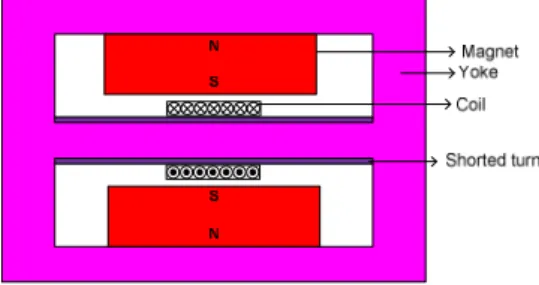
In a voice coil motor, the actuation force to a moving part is directly proportional to the coil current. Therefore, it is desired that the current rises quickly and shorten the access time to expedite system response. One way to accomplish this condition is to place a copper tube (shorted turn) concentric to the moving coil as shown in Fig. 3.1. When a voltage is applied to the coil, flux in the magnet circuit induces a high current in the copper sleeve in such a way as to retard the increasing flux. The result is that an effective inductance seen by the coil is drastically reduced, thus making the coil act more like a resistive element instead of a resistance-inductance circuit. As a consequence, the current rises quickly, providing a greater actuation force right from the start.

Fig. 1. VCM with shorted turn.

A. Shorted Turn Model

Fig. 2 depicts a shorted turn model based on a transformer circuit. According to Kirchhoff’s law in Fig. 2(d), we may obtain electric circuit equations

12 11 12 ( / ) ( ) ( ) ( ) c s ( ) c c c v di d i e t R i t L L L K v t dt dt α = + + − + (1) 2 12 12 22 ( / ) 0 ( / ) c ( ) s s s di d i R i L L L dt dt α α α = − + + (2)

where the quantities with the subscript

c

refer to those for the

primary coil and

s

refer to those for the shorted turn,

e

_c is

the input voltage for the primary coil,

R

_c is the primary coil

self-inductance of the primary coil,

L

₁₂ is the mutual inductance

between the primary coil and the shorted turn,

K

_v is voltage

constant,

v t

( )

is the velocity of the movable coil,

R

_s is the

shorted turn resistance,

L

₂₂ is the self-inductance of the

shorted turn,

i

_s is the current in the shorted turn, and

/

c s

N

N

α

=

is the turn ratio of the primary coil and the

shorted turn.

The coil current builds up rapidly even before the coil has time to build up its speed. Therefore, to study the effect of the shorted turn in the initial coil current rise, we can safely

neglect the term

K v t

_v

( )

in Eq. (1). Rewriting Eq. (3.1)

without the term

K v t

_v

( )

, we obtain

12 11 12 ( / ) ( ) ( ) ( ) c s c c c di d i e t R i t L L L dt dt α = + + − (3)

Eqs. (2) and (3) show that they are exactly the same as transformer equations with the shorted turn. Therefore, the effects of the shorted turn can be conveniently studied by using a transformer model in Fig. 2 where the coil is considered as the primary circuit and the shorted turn as the secondary. N + -Rc ic is Ns Rs 12 φ 22 φ 11 φ Magnetic circuit

(a) Schematic diagram of transformer

12 ρ 11 ρ ρ22 11 φ φ12 φ22 Nic Nsis

(b) Magnetic equivalent circuit

Ec Ec + -ic Rc Lc Ls _Rs is M

(c) Equivalent circuit for shorted turn

Ec -ic Rc L11 L22 N2_R s is/N L12

(d) Equivalent circuit referred to primary side

Fig. 2. Shorted turn model based on transformer circuit.

Solving Eqs. (2) and (3) that are subjected to a step voltage

c

E

in

e t

_c

( )

gives general solutions written as

2 - 2 - 2 - -2 11 1 11 2 12 1 12 12 2 - - - -1 12 2 12 12 2 1 1 2 1 1 ( ) - [ -2 - - 2 - - - ] Bt At Bt At c s s s c c At Bt Bt At At Bt s c c s c s c i t C R L e C R L e C R L e C L R e L R C R L e C L R e L E C L R e C L R e C e D C e D α α α α α α = + + + + ⋅ ⋅ 1 2 ( ) At Bt s i t ₌C e− ₊C e−

Substituting initial values

i

_c

(0) 0, (0) 0

=

i

_s

=

yields

2 2 11 12 12 22 2 2 11 12 12 22 ( ) [1 2 ] 2 At c s c s c c c Bt s c s c E R L L R R L L R D i t e R D R L L R R L L R D_e D α α α α − − − + − + = − − + − − + (4) 12 ( ) c( At Bt) s L E i t e e D α − − = − (5) where 2 2 12 22 12 11 12 11 22 12 11 22 2 2 12 22 12 11 12 11 22 12 11 22 2 2 2 2 2 2 2 2 2 12 12 22 12 12 11 22 22 12 2 2 22 11 12 2( ) 2( ) ( 2 2 2 2 2 c c s s c c s s c c c s c s c c s c s s R L R L R L R L D A L L L L L L R L R L R L R L D B L L L L L L D L R L R L L R R L R R L L R L R R L L R R L R L α α α α α α α α α + + + − = + + + + + + = + + = + + − + − − + ４ 1 2 4 2 4 2 2 2 12 11 11 2α R L Ls α R Ls ) + +

B. Derivation of VCM Model with Shorted Turn

Carrying out Laplace transform in Eqs. (2) and (3) gives

12 12 11 ( ) ( ) ( ) ( ) ( ) c c c c s L e s R i s L L si s si s α = + + − (6) 12 22 12 0 s s( ) c( ) s( ) L L R i s L si s si s α α+ = − + (7) According to Eq. (7), 12 2 12 22 ( ) ( ) ( ) s c s L s i s i s R L L s α α = + + (8)

Substituting Eq. (8) into Eq. (6) yields

2 2 2 2 12 22 11 12 11 22 11 12 12 22 2 12 22 ( ) ( ) ( ) ( ) ( ) c s s c c c s c s e s L L L L L L s R L R L R L R L s R R i s R L L s α α α α + + + + + + + = + + (9)

By Newton’s second law, the equation of motion is written as

2 _{( ) ( )} ( ) f c d x t dx t m b K i t dt + ⋅ dt = ⋅ (10)

whose Laplace transform leads to

2 ( ) ( ) f c k x s i s =ms +bs (11)

Thus, Eqs. (9) and (11) lead to the transfer function for VCM with shorted turn

2 12 22 2 2 2 2 12 22 11 12 11 22 11 12 12 22 [( ) ] ( ) ( ) ( )[( ) ( ) ] f s c s s c c c s k L L s R x s e s s ms b L L L L L L s R L R L R L R L s R R α α α α + + = + + + + + + + + (12)

C. VCM with Shorted Turn Magnetic Field Analysis

In previous sections, we have discussed various aspects of linear voice coil motors with shorted turn. In Section 3.4, we will introduce VCM with shorted turn magnetic field analysis and use the software Ansoft Maxwell to conduct finite element analysis.

The Maxwell field simulator is an interactive software package that uses finite element analysis to solve magnetic problems. The Maxwell software then does the following.

Automatically creates the required finite element mesh to calculate the desired magnetic field solution and special quantities of interest, such as force, torque, inductance, capacitance, or power loss. Dividing a structure into many smaller regions (finite elements) allows the system to compute the field solution separately in each element.

A VCM is shown in Fig. 3, which includes yoke, shorted turn, primary coil and magnets. The magnetic design includes a copper tube (shorted turn) in the outer moving coil. Therefore, the third-type voice coil motor has advantages, a good magnetic shielding, great magnetic flux density and large thrust force. In the VCM, the coil has 200 laps. The coil resistance and current are 7.9Ω and 6A, respectively. The thrust force of coil is calculated as 1.027N. The mass of moving parts (the coil and the lens holder) are 5.65g and the shorted turn is 6.36g. The thrust force is sufficient to overcome gravity to make the moving part move. Flux lines of this VCM design are shown in Fig. 4. Magnetic field distribution and magnetic-flux density distribution are shown in Figs. 5 and 6, respectively.

Fig. 3. Magnetic circuit schematic of this design.

Fig. 4. Flux lines of this VCM design.

Fig. 5. Magnetic field distribution of this VCM design.

Fig. 6. Magnetic-flux density distribution of this VCM design.

III. SLIDING MODE APPROACH TO FUZZY CONTROL

This study creates a linguistic system to design fuzzy control, for which sliding modes are used to determine parameters in control rules.The design procedure is to first

specify the response

P

_d

(

e

,

ec

)

on the phase plane and then

design a fuzzy controller to achieve this response. To carry out the fuzzy control method, control action is formulated on a partition plane depicted in Fig. 7. Finally, values of 12

parameters

p

i_j,

i

=

1 …

,

,

4

,

j

=

0

,

1

,

2

are determined such

that both desired reaching and sliding conditions can be

satisfied to ensure robustness. To determine these values,

D

_r,

r

E

, and

F

_r,

r

=

1

,

3

,

7

,

9

are made equal to 12 parameters

i j

p

. In addition, control actions in these four regions are

linear functions that facilitate the determination of parameters. Control actions in the four quadrants can be written as

u

=

Θ

_crΤ

w

_c (13)

where _ΘcrΤ ₌

[

D_r E_r F_r

]

_{, r=1 ,3 ,7,9, and w}

[

_{e ec}

]

cΤ=1 . cr

Θ

consists of elements

p

i_j. Moreover, switching functions

are defined as

ec

e

s

=

λ

+

(14)

which is shown in Fig. 7, where

λ

is a positive constant. It is

seen that the switching function is located in the second and

fourth quadrants. From Eq. (14), error

e

=

x

−

x

_d, where

x

denotes the current value,

x

_d denotes the target value. And

error change

ec

denotes the current error minus the error at

the previous time. If the time is vary short,

ec

can take as the

slope of

e

. In other words,

ec

can take as

e

. Therefore, Eq.

(14) becomes

e

e

s

=

+

_λ

(15) If

t

→

∞

, and

e

→

0

,

x

( )

t

→

x

_d

( )

t

. e ec P X e= ~ e=XN~ N X ec= ~ P X ec= ~ e e s= +λ Fig. 7. Switching function s on phase plane.

In this study,

x

denotes the current displacement,

x

_d

denotes the target displacement. To achieve precise position control, where the target displacement is 1mm in the system.

Therefore,

e

denotes the current amplitude,

e

denotes the

because

s

=

0

denotes that

e

=

0

and

e

=

0

. It means there is precise position control in the system, which is the ideal condition. Hence, we observe the trajectory on the phase plane

(

e

e

)

P

_d and observe the trajectory if convergence to origin

following switching function

s

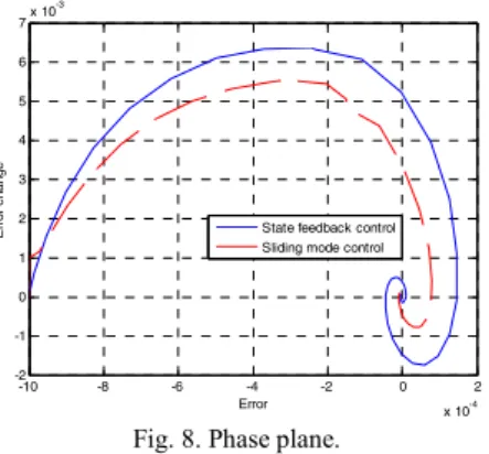
in short time. First, we

observe the phase trajectory as sliding mode control off and control on. Fig. 8 shows the phase trajectory when using sliding mode control.

-10 -8 -6 -4 -2 0 2 x 10-4 -2 -1 0 1 2 3 4 5 6 7x 10 -3 Error E rr o r c h a nge

State feedback control Sliding mode control

Fig. 8. Phase plane.

Presently, this study uses the switching function

s

and

employs the converge speed of phase trajectory to the origin

along a switching function

s

. And parameters of fuzzy

control in are determined. The control block diagram is shown

in Fig. 9. Since positive

( )

P

~

and negative

( )

N

~

are denoted as

fuzzy subsets for input variables, four fuzzy rules can be written as

IF

e

is

P

~

AND

e

is

P

~

, THEN

u

=

p

1₀

+

p

₁1

e

+

p

1₂

e

IF

e

is

P

~

AND

e

is

N

~

, THEN

u

=

p

₀2

+

p

₁2

e

+

p

2₂

e

IF

e

is

N

~

AND

e

is

P

~

, THEN

u

=

p

₀3

+

p

₁3

e

+

p

3₂

e

IF

e

is

N

~

AND

e

is

N

~

, THEN

u

=

p

₀4

+

p

₁4

e

+

p

4₂

e

In the above four rules, 12 parameters

p

i_j in the consequence

are determined by sliding mode theory. I set the fuzzy subset and tuned the parameters to satisfy the sliding mode theory. Displacement curves in simulation results are shown in Figs. 10. The fuzzy control method is based on the sliding mode theory, but the simulation result is not good. The reasons are described as follows: Sliding mode control can provide input independent according to the states feedback at that time. If the states are changed, input can be changed immediately. But in sliding-mode-based fuzzy control fuzzy subsets are used to divide states and input into many regions. This work employs states subsets to determine output subsets. Hence, the input of sliding-mode-based fuzzy control is not as accurate as like sliding mode control. Accordingly, the reduction effect is worse than sliding mode control. Hence, simulation results

show that both methods arrive at the goal with comparable accuracy. A B s 1 u ₊₊ x x H y i j p

Fig. 9. Block diagram of sliding-mode-based fuzzy control.

0 0.1 0.2 0.3 0.4 0.5 0.6 0.7 0.8 0.9 1 -2 0 2 4 6 8 10 12x 10 -4 Time (s) D isp la ce m e n t ( m

) Sliding-Mode-Based Fuzzy Control_{Sliding mode control}

Fig. 10. Comparison of displacement results using two control methods.

IV. EXPERIMENTAL RESULT

A. Experimental Setup

The experiment apparatus includes power supply, oscilloscope, laser displacement sensor, VCM, and PC. In the experiment, we use power supply and provide DC voltage 2.0V to 4.5V to try displacement of moving part of VCM. Fig. 11 shows the laser displacement sensor which measures displacement signal of moving part of VCM through the laser.

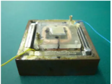
Fig. 11. Laser displacement sensor measures displacement signal. In VCM with shorted turn design and manufacture aspects, the magnetic design is based on the third design of Fig. 2.5 and we place a copper tube (shorted turn) in the outer moving coil. The cross section of lateral VCM with shorted turn and the VCM mechanism design are shown in Figs. 12 and 13. The VCM photo is shown in Fig. 14 that includes lens foundation, coil, shorted turn, yokes and permanent magnets. The VCM sizes are about four times of an actual product. Concerning materials, lens foundation, coil, shorted turn, yokes and permanent magnets use acryl, 200 laps AWG37

copper wire whose diameter is 0.113mm, copper, iron and N48H (NdFeB).

Fig. 12. Cross section of lateral VCM with shorted turn.

Fig. 13. Mechanism design of VCM with shorted turn.

Fig. 14. Photo of VCM with shorted turn.

B. Measurement Result

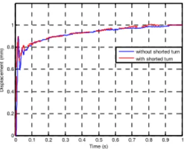
In the experiment apparatus, the voice coil motor is turned on using a switch in power supply, which provides voltage to VCM. By adjusting input voltage, this study compares VCMs without and with shorted turn. Figs. 15 and 16 show measurement results in step response when input voltages are 2.5V and 3.0V, respectively. Hence, it is concluded that the stroke of VCM with shorted turn is larger than without shorted turn when supply voltages are the same. Because of the design of shorted turn, the moving part of VCM can have a greater stroke in the transient response.

0 0.1 0.2 0.3 0.4 0.5 0.6 0.7 0.8 0.9 1 0 0.1 0.2 0.3 0.4 0.5 0.6 0.7 0.8 0.9 1 Time (s) D isp la ce m e n t ( m m )

without shorted turn with shorted turn

Fig. 15. Measurement result in step response when input voltage is 2.5V.

0 0.1 0.2 0.3 0.4 0.5 0.6 0.7 0.8 0.9 1 0 0.1 0.2 0.3 0.4 0.5 0.6 0.7 0.8 0.9 1 Time (s) D is p la c e me n t (

mm) without shorted turn

with shorted turn

Fig. 16. Measurement result in step response when input voltage is 3.0V.

C. Control Experiment Result

The control block diagram is shown in Fig. 17. The control method is computed in PC, and through AD/DA card output voltage to the diver (current amplifier) to drive the VCM. The moving part of VCM is moved by electromagnetic force. A laser displacement sensor is used to measure displacement and transfer acquisition data to a personal computer. Figs. 18 and 20 show positioning control experiment result of stroke 0.8mm and input signal measurement result. Fig. 19 shows experimental result of 0.8mm stroke which extends time axis to steady state. Figs. 21 and 23 show positioning control experimental result (1.0mm stroke) and input signal measurement result. Fig. 22 shows positioning control experiment result (1.0mm stroke) which extend time axis to steady state. We conclude that responses of VCM with shorted turn and without shorted turn are both similar, but VCM with shorted turn can arrive at the same location by lower input signal.

0 0.1 0.2 0.3 0.4 0.5 0.6 0.7 0.8 0.9 1 0 0.1 0.2 0.3 0.4 0.5 0.6 0.7 0.8 0.9 1 Time (s) D isp la ce m e n t ( m m

) without shorted turn

with shorted turn

Fig. 18. Experimental result (0.8mm).

0 0.2 0.4 0.6 0.8 1 1.2 0 0.1 0.2 0.3 0.4 0.5 0.6 0.7 0.8 0.9 1 Time (s) D isp la ce me n t ( m m

) without shorted turn

with shorted turn

Fig. 19. Experimental result (0.8mm).

0 0.1 0.2 0.3 0.4 0.5 0.6 0.7 0.8 0.9 1 0 0.5 1 1.5 2 2.5 3 3.5 4 4.5 5 Time (s) V o lt age ( V )

without shorted turn with shorted turn

Fig. 20. Input signal measurement result (0.8mm).

0 0.1 0.2 0.3 0.4 0.5 0.6 0.7 0.8 0.9 1 0 0.2 0.4 0.6 0.8 1 Time (s) D is p la c e m ent ( m m

) _{without shorted turn}

with shorted turn

Fig. 21. Experimental result (1.0mm).

0 0.2 0.4 0.6 0.8 1 1.2 0 0.2 0.4 0.6 0.8 1 Time (s) D isp la ce m e n t ( m m )

without shorted turn with shorted turn

Fig. 22. Experimental result (1.0mm).

0 0.1 0.2 0.3 0.4 0.5 0.6 0.7 0.8 0.9 1 0 0.5 1 1.5 2 2.5 3 3.5 4 4.5 5 Time (s) V o lt age ( V )

without shorted turn with shorted turn

Fig. 23. Input signal measurement result (1.0mm).

V. CONCLUSION

This study has proposed a new voice coil motor design. The design places a copper tube (shorted turn) in the outer moving coil, and it can make the coil current to rise quickly, providing a greater accelerating force right from the start. According to experimental results, both response curves of VCMs with and without shorted turn are close to each other, but the VCM with shorted turn can reach the same location under smaller input voltage.

REFERENCES

[1] Wagner, J. A., “The Shorted Turn in the Linear Actuator of a High Performance Disk Drive”, IEEE Transactions on Magnetics, Vol. MAG-18, No. 6, pp. 1770-1772 , 1982.

[2] Wagner, J. A., “The Actuator in High Performance Disk Drives: Design Rules for Minimum Access Time”, IEEE Transactions on Magnetics, Vol. MAG-19, No. 5, pp.1686-1688 , 1983.

[3] Barton, R. K., “Eddy Current and Skin Effect in Edgewise Wound Copper Coils”, IEEE Transactions on Magnetics, Vol. 25, No. 4, pp. 3016-3018, 1989.

[4] Moser, M.A., “Shorted Turn Effects in Rotary Voice coil Actuators”, IEEE Transactions on Magnetics, Vol. 32, No. 3, pp. 1736-1742 , 1996.