Efficient Cluster Radius and Transmission Ranges in Corona-based Wireless Sensor Networks

(1)

Efficient Cluster Radius and Transmission

Ranges in Corona-based Wireless Sensor

Networks

Wei Kuang Lai1, Chung-Shuo Fan2* and Chin-Shiuh Shieh3

1 _{Department of Computer Science and Engineering, National Sun Yat-Sen University} Kaohsiung 804 - Taiwan

[e-mail: wklai@cse.nsysu.edu.tw] 2

Department of Computer Science, National Chiao Tung University Hsinchu 300 - Taiwan

[e-mail: csfan@g2.nctu.edu.tw] 3

Department of Electronic Engineering, National Kaohsiung University of Applied Sciences Kaohsiung 807 - Taiwan

[e-mail:csshieh@cc.kuas.edu.tw] *Corresponding author: Chung-Shuo Fan

Received December 2, 2013; revised February 6, 2014; accepted March 14, 2014; published April 29, 2014

Abstract

In wireless sensor networks (WSNs), hierarchical clustering is an efficient approach for lower energy consumption and extended network lifetime. In cluster-based multi-hop communications, a cluster head (CH) closer to the sink is loaded heavier than those CHs farther away from the sink. In order to balance the energy consumption among CHs, we development a novel cluster-based routing protocol for corona-structured wireless sensor networks. Based on the relaying traffic of each CH conveys, adequate radius for each corona can be determined through nearly balanced energy depletion analysis, which leads to balanced energy consumption among CHs. Simulation results demonstrate that our clustering approach effectively improves the network lifetime, residual energy and reduces the number of CH rotations in comparison with the MLCRA protocols.

Keywords:Wireless sensor networks, clustering, sensors, load balancing, cluster head

This work was supported in part by the National Science Council, Taiwan, ROC under the grant Nos. 100-2221-E-151-041-, 101-2219-E-110-001- and 100-2219-E-110-001-.

(2)

1. Introduction

W

ireless sensor networks (WSNs) have a wide range of applications, such as environment monitoring [1]–[3], security [4], [5], military sensing, home automation, healthcare [6] and traffic surveillance [7], etc. A typical WSN comprises a sink node and a large number of sensor nodes. A sensor node is in general of small sized and capable of sensing and communicating. However, sensor nodes are generally powered by batteries. Energy becomes one of the most critical issues in WSNs as these sensor nodes are non-rechargeable in most cases.

It is well recognized that cluster architecture can save more energy and therefore increase the network lifetime. In a typical two-tier WSN, the information is aggregated at the cluster head (CH) and then be transmitted to the sink via multi-hop communications. The concept of clustering is advantageous for both intra-cluster data collection and inter-cluster data forwarding, since the transmission ranges, as well as power consumption, in both case can be substantially reduced.

Aimed at balanced power consumption, numerous cluster-based approaches have been studied. However, to the best of our knowledge, none of existing protocols contributes directly to the determination of appropriate cluster radius of each corona in corona-structured WSNs. To this issue, we introduce a novel cluster-based routing protocol called “ECT” (Efficient Cluster radius and Transmission ranges in corona-based WSNs), which determines the cluster radius for each corona according to the traffic load imposed on its CH. The main contributions of this paper are listed as follows.

(1) Calculating the cluster radius for each corona according to the energy

consumption of CHs.

This will prevent the overloading of CHs close to the sink. That is, relaying load is evenly allocated to CHs so that the CHs near the sink do not run out their power far earlier than others.

(2) Adopting cross-corona transmissions for extend network lifetime.

When the sensor nodes in cluster CSi,j, where i represents the ith corona and j denotes the

order of the cluster in that corona, can no longer serve as a CH, the CHs in corona Ci+1 take

charge of cross-corona data transmissions. In this way, the network lifetime can be effectively extended.

The rest of this paper is organized as follows. Section 2 surveys some related works. Section 3 presents the assumptions and observations. Section 4 explains how cluster radius can be determined according to the demand of relaying traffic. The proposed method ECT is explained in detail in Section 5. In Section 6, we discuss the simulation results. Finally, Section 7 concludes this paper.

2. Related Work

A number of clustering schemes [8]–[12] are proposed for the purpose of equalizing the energy consumption among all sensor nodes. Li and Mohapatra [13] investigate the validity of various possible methods to alleviate the energy hole problem. It has been noted that in a uniformly distributed WSN, hierarchical deployment has its benefits. Heinzelman, et al. [14] propose a CH rotation approach called LEACH. It picks out CHs randomly while each sensor node takes turns to serve as the CH in order to achieve energy-balancing. LEACH assumes

(3)

that every node within the network is capable of reaching the sink directly. Deterministic cluster-head selection (LEACH-DCHS) [15] improves LEACH by taking the residual energy of the sensor node into consideration in the threshold function. This scheme ensures that the sensor node with more energy has a larger opportunity to be a CH. Ye, et al. [16] propose a distance-based cluster formation method (called EECS) with unequal cluster size in single-hop WSNs. Cluster sizes closest to the sink are larger while those located away from the sink are smaller. Therefore, CHs far from the sink can reserve more residual energy for long-distance data transmission to the sink. However, single-hop transmission consumes more energy than multi-hop communications. Lian, et al. [17] examine static models with uniformly distributions of sensor nodes for large-scale WSNs. At the end of the network lifetime, there is still considerable amount of residual energy, which can be up to 90 percent of total initial energy. Therefore, the static models with uniformly distributed sensor nodes fail to utilize their energy effectively. However, we demonstrate that nearly balanced energy depletion can be achieved with the help of carefully planned cluster radius and transmission ranges.

We here introduce a typical approach, which is compared to our proposed ECT scheme. Liu, et al. [18] propose a novel clustering scheme integrating hierarchical clustering on the basis of classical routing algorithm, which is called Multi-Layer Clustering Routing Algorithm (MLCRA). First of all, each sensor node broadcasts its own information within one hop to set up neighbor lists. This algorithm relies on probability (based on LEACH-DCHS) to determine whether a sensor node is a CH (first-class CH) or not. The chosen CH then broadcasts a CH_message that contains the node ID, residual energy, the layer number of the node and the distance to the sink node. Each sensor node receives a CH_message to check whether the layer number of the received CH_message belongs to its upper layer or not. If yes, it stores the information of the sensor node to the candidate list (first-class clusters formed); otherwise, it discards the received message. Sensor nodes in the candidate list can be chosen as the CH (second-class CH) based on the following two cases. If a sensor node is in the first level, the sensor node with the maximum ratio (i.e., the ratio of (the node's residual energy) to (the distance to the sink)) is selected as the CH (second-class CH). On the other hand, if the node is not in the first level, the sensor node in the candidate list (closest to the sink) is chosen as the CH (third-class CH). The process continues until the k-class CHs selected and the k-class clusters formed (the entire network topology is covered). Sensor nodes in the first-class clusters adopt direct communications, and the non-first-class CHs use multi-hop communications. Simulation results show that the MLCRA protocol achieves considerable improvement in network lifetime compared to the LEACH and LEACH-DCHS schemes.

3. Preliminaries

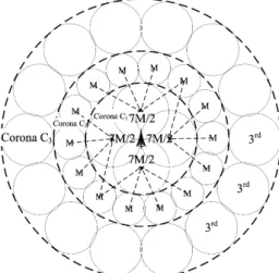
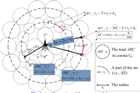
We consider a circular area of radius R with a static sink located in the center. Sensor nodes are uniformly distributed in topology. A corona model is used by partitioning the circular area into several coronas. The ith corona is denoted by Ci. A corona Ci is further divided into several

cluster CSi,j with the same cluster radius (ri), where i represents the ith corona and j donotes the

order of the cluster in that corona, as shown in Fig. 1 (note that Fig. 1 is only an illustration of corona model, actual cluster radius in each corona will be calculated later in Section 5.1). Moreover, following are one theorem and two observations that can be further used in Section 4.

(4)

Fig. 1. An illustration of 3-corona model Theorem 1. The deviations (

∆

_i) is defined as arc_ri / (2×ri ), then

}

)

4 sin(

2 {

}

360 {

o i o i i

θ

π

×

=

∆

. (1)

The proof is given in Appendix.

Observation 1. When θi-1∈ [10°,120°] and θi∈ [10°,120°], for two arbitrary deviations

∆

i−1 and

∆

_i, their ratio

i i

∆

₋₁

have a value close to 1 (i.e.,

0 .

95

1

≤

1 .

05 ∆

∆

≤

− i i ). That is

i

i i

≈

∀

∆

₋

,

1

1 . (2)

Proof. According to Theorem 1, even when the difference between θi-1 and θi is obvious (i.e.,

θi-1 =10° and θi =120°), the value of i i

∆

₋₁

is very close to 1 (i.e.,

).

1 955233

.

0 }

)

4

10 sin(

360

120 {

}

)

4

120 sin(

360

10 {

}

)

4 sin(

2

360 {

}

)

4 sin(

2

360 {

1 1 1

=

≈

×

=

×

=

∆

− − − o o o i o i o i o i i i

θ

π

θ

π

(5)

Fig. 2 shows all values for any θi and θi-1 between 10° and 180°. Therefore, we can simply

assert that this observation is right based on Fig. 2.

Fig. 2. The ratio of

∆

_i₋₁ to

∆

_iwhen θi-1

∈

[10°, 180°] and θi

∈

[10°, 180°]

Observation 2. For two arbitrary ai and aj (the number of clusters in corona Ci and corona Cj), its ratio can be expressed as

. , ) 2 ( ) 2 ( 2 1 1 1 1 1 1 i r r r r r r a a i k i k i i k i k i i i ∀ + × + × =

∑

− = − − = − − (3) Proof.

Let ARC_ri be the total circumference of the circle in corona Ci (as shown in Fig. 1),

therefore

,

)

2 (

2 _

),

(

2 _

r

₁

r

₁

ARC

r

₂

r

₁

r

₂

ARC

=

π

×

=

π

×

+

,

_

2 (

2 ).

1 1 i i k k i

r

ARC

=

×

∑

+

− =

π



(4)

Let arc_ri be a part of the arc in corona Ci (which is equal to 2×ri×Δi, as shown in Theorem 1

and Fig. 1). We can have arc_ri divided by ARC_ri to roughly calculate the ai .









∆

×

+

×

≈









∆

×

+

×

≈









∆

×

≈

∑

− = i i i i k k i

r

a

r

a

r

a

2 )

2 (

2 ,

,

2 )

2 (

2 ,

2

1 1 2 2 2 1 2 1 1 1 1

π



(5)

, where Δi is the deviations (as mentioned before). Based on (5) and Observation 1

(i.e., 1

≈

1 ∆

∆

₋ i i _{), then} i r r r r r r a a i k i k i i k i k i i i ∀ + × + × =

∑

− = − − = − − , ) 2 ( ) 2 ( 2 1 1 1 1 1 1

. This completes the proof of this

(6)

4. Balanced Energy Depletion Analysis

According to the radio energy dissipation model in [19], the transmission energy for l bit of data over a distance d is ETx(l,d)= l×(Eelec +εamp×d2), where Eelec is the energy used in a sensor node for transmitting one bit of data, εamp is the amplifier energy (multi-path model) and d

refers to the maximum transmission distance. Note that various energy dissipation models can be used in the following derivations. That is, our scheme can be applied to different models. We use the radio energy dissipation model as an example because it is a typical model in WSNs.

Assume that each cluster member transmits 1 bit of data to its CH. Let D and CHi,j are the

density of the sensor nodes (uniformly distributed) and the CH belongs to CSi,j, respectively.

Basically, each CH (CHi,j) in outermost corona Ci only takes care of the data transmitted by its

own cluster members (i.e.,

π

×

r

_i2

×

D

). However, the CHs in corona Ci-1 not only handle the

data transmitted by their own cluster members, but they also relay packets from corona Ci

(i.e., 1 2 2 1 − − × + × × × × i i i i a a D r D r

π

), where ai be the number of clusters in corona Ci. The

distance between the centers of two clusters is regarded as the transmission range for simplicity (i.e., (ri+ri-1) in corona Ci, (ri-1+ri-2) in Ci-1 and so on). In addition, the distance

between each CH1,j (in innermost corona C1) and sink is only r1. Applying Observation 2, the total energy consumption of a CH in corona Ci can be evaluated as follows.

                                  × + × + × × × + × = + × + × + × + × × × + + × + × × × + × = + × + × + × + × × × + × = + × + × × =

∑

= − = − − − = − − = − − = − − − = − − − − − − − − = − − = − − − − i p amp elec p p k p k p i i amp elec i k i k i i k i k i i i k i k i i k i k i i i i i i amp elec i k i k i i k i k i i i i i i amp elec i i r E r r r D r D r E r r E r r r r r r D r r r r r r r D r D r E r r E r r r r r r D r D r E r r E D r E 2 2 1 1 1 2 2 1 1 2 3 2 3 1 2 1 1 2 2 3 1 2 1 2 1 1 2 2 1 2 2 2 2 2 1 2 1 1 1 1 1 2 2 1 1 2 1 2 ] [ ) 2 ( ] ) ( [ )] ) 2 ( ) 2 ( ( ) ) 2 ( ) 2 ( ( ) [( ] ) ( [ )] ) 2 ( ) 2 ( ( ) [( ] ) ( [ ) ( ε π π ε π π π ε π π ε π 

(6)

To balance the energy consumption among CHs, we apply (7) to calculate the cluster radius for each corona.

(7)







=

×

+

×

+

×

+

×

≈

− −

R

r

E

i i i i

2

₁ ₂ ₁ 1 2 1



(7)

, where R is the radius of the whole topology.

5. ECT

The ECT scheme consists of three phases, namely cluster formation phase, data forwarding phase and cluster maintenance phase.

5.1 Cluster Formation Phase

The cluster formation phase consists of the number of coronas in network topology, the cluster radius, cluster setup and CH-to-CH transmission capacity.

 The Number of Coronas in Network Topology

First of all, the sink divides the network topology into K-coronas. The cluster radiuses within the same corona are equal. Clusters closest to the sink grouped in the 1st corona and so on. The clusters located farthest from the sink are put in the Kth corona (as shown in Fig. 1).  Cluster Radius

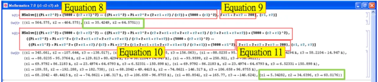
As stated before, the cluster radius in each corona can be calculated using (6) and (7). More specifically, two numerical examples for 2-corona and 3-corona model are illustrated. The ratio of r1, r2 and r3 can be obtained by (8) and (10). By substituting the obtained ratio into (9) and (11), actual cluster radius in each corona (i.e., r1, r2 and r3) can be calculated.For the purpose of clarity, we detailed descript how to solve Equations 8, 9, 10 and 11 by using Mathematica [20], as shown in Fig. 3. It is easy extend this example to the k-corona model. Table 1 shows the variation of the cluster radius (ri) with various network radii (R) ranging

from 200m to 600m. It also provides the guideline for designing the cluster radius in WSNs.

       ≈ × + × × + × × × × + × × = + × + × × × = 2 1 2 1 1 2 2 1 1 2 2 2 1 1 2 1 2 2 2 2 ] ) ( [ )] ) ( ) 2 ( ( ) [( ] ) ( [ ) ( E E r E r r r r r D r D r E r r E D r E amp elec amp elec

ε

π

ε

π

(8)

200

2

2 r

₁

+ r

₂

=

(9)                ≈ ≈ × + × + + × × × + + × × × + × × = + × + × + × + + × × × × + × × = + × + × × × = 3 2 1 2 1 3 3 2 1 2 3 2 2 1 2 2 2 1 1 2 1 2 2 1 3 3 2 1 2 2 3 2 2 2 2 2 3 2 3 3 ] ) ( [ )] 2 2 ( ) 2 ( ) [( ] ) ( [ )] ) 2 ( ) 2 2 ( ( ) [( ] ) ( [ ) ( E E E r E r r r r D r r r r D r D r E r r E r r r r r r r D r D r E r r E D r E amp elec amp elec amp elec

ε

π

ε

π

ε

π

(10)

200

2

2 r

1

+

r

2

+

r

3

=

(11)

(8)

Fig. 3. Using Mathematica to solve Equations 8 and 9

Table 1. Computational results for 2-corona, 3-corona and 4-corona models

 Cluster Setup

The sensor nodes broadcast their own information with each other; the one with the most central location (minimum euclidean distance in each cluster) in each cluster serves as a CH. The chosen CH broadcasts a Head_Msg within its transmission range. This message contains current energy level, the distance between the CH and sink, and the sensor node’s ID, which is used as the cluster’s ID as well. If a sensor node receives multiple Head_Msgs, the sensor node selects and joins the closest CH. For those sensor nodes that do not serve as CHs and do not receive any Head_Msg, they may send a Find_Msg to seek the closest clusters to join them.

 CH-to-CH Transmission Capacity

After clusters are setup, the sink can calculate the number of clusters in each corona based on the cluster radius. Once ai is obtained (as mentioned before), we have the number of

clusters in corona Ci divided by the number of clusters in corona Ci-1.

) 2 ( ) 2 ( 1 1 1 1 j j p p i i i k k j i j r r r r r r S + × + × =

∑

− = − = (12)

(9)

Fig. 4. Unequal amount of transmission capacity between two CHs

Fig. 5. Equal amount of transmission capacity between two CHs

In some cases, the transmission capacity of CHs may be unequally arranged (as shown in Fig. 4, the transmission capacity of some clusters in corona C1 are 3×M2, others are 4×M2). Accordingly, the transmission capacity of each CH may be well adjusted to balance its sharing (as shown in Fig. 5, each cluster in corona C1 has an equal amount of transmission capacity of 14×M2/4).

5.2 Data Forwarding Phase

The data forwarding phase consists of intra-cluster and inter-cluster data forwarding.  Intra-Cluster Data Forwarding

In this phase, we adopt the MST [21] to shorten the distance of data transmission between sensor nodes and CHs. When a network has high density of sensor nodes, the transmitted information may take a long time before reaching the targeted CHs. Therefore, a hop count H is assigned. Once the sensor nodes proceed to forwarding data, the value of H is decreased by one. When the value of H is equal to zero and the data do not reach the targeted CH yet, the sensor node holding the data at the time directly transmit data to the CH to avoid time-consuming routing.

(10)

 Inter-Cluster Data Forwarding

In this phase, CHs in corona Ci receive data from designated CHs in corona Ci+1, and then

transmit data to the next adjacent CHs in corona Ci-1 (closest to the sink); the process keeps on

going until the data finally reaches the sink.

5.3 Cluster Maintenance Phase

 CH Rotations in a Cluster

A lot of typical clustering protocols reselect CHs per round so that the loads can be shared among all sensor nodes. However, frequent CH rotations impose considerable overheads since all cluster members have to be notified about the changes. In order to avoid such scenario, this phase defines the threshold of CH power as T. Note that CH rotation is triggered only when the residual energy of original CH is below a threshold T. Specifically, if the residual power of the CH is under T, the sensor node closest to the CH is elected as the new CH in the cluster. Meanwhile, new CH broadcasts the Change_Msg to notify its cluster members.

 Cross-Corona Data Transmissions

When each sensor node in cluster CSi,j is no longer serve as a CH, the CHs in corona Ci+1

implement cross-corona data transmissions (as shown in Algorithm 1). In this way, the network lifetime can be prolonged.

Algorithm 1: Cross-corona data transmissions

1. Begin

2. For all i = k to 1 // For each corona 3. For each CH in corona Ci, pass data to CH in Ci-1

// Ck… C1C0 , C0 represents the sink

4. Repeat

5. if (the residual energy of CH in corona Ci is under T) // T: the threshold of CH power

6. pick out a new CH // closest to the original CH within its cluster

7. While (the power of each sensor node in Ci is under T)

8. {For each cluster in Ci+1, pass data to the sink directly

// cross-corona data transmissions

9. } // End While

10. Until (residual energy of first sensor node is depleted)

11. End // End Begin

6. Simulations

We evaluate the performance metrics of ECT and compared it with MLCRA protocol. We choose MLCRA [18] as a comparison reference because MLCRA is one of the most recent clustering algorithms proposed in the literature. It achieves much improvement in the network lifetime when compared to LEACH [14] and LEACH-DCHS [15]. All the parameters are given as follows: The network radius ranges from 200m to 600m; Eelec = 50 nJ/bit, εamp = 10 pJ/bit/m2; Energy dissipation of CH rotation is 0.02 mJ; each sensor node has an initial energy of 1 joule; 500 sensor nodes are uniformly distributed in topology; each sensor node sends 400 bits of data per unit time to the sink via multi-hop communications. Besides, sensor nodes can adjust the transmission ranges, the maximum transmission range can be used in transmitting data to the sink directly. We average the results of 200 runs for each scenario.

(11)

1) network lifetime [14]; 2) residual energy; and 3) the number of CH rotations.

The network lifetime is defined as the time until first sensor node uses up its energy and is measured in “round”. The definition of a round is that one packet is transferred from the sensor node via the CH to the sink. The number of CH rotations indicates the total number of cluster head rotations before the network operation ends.

6.1 Network Lifetime

Fig. 6. Network lifetime comparison between ECT and MLCRA

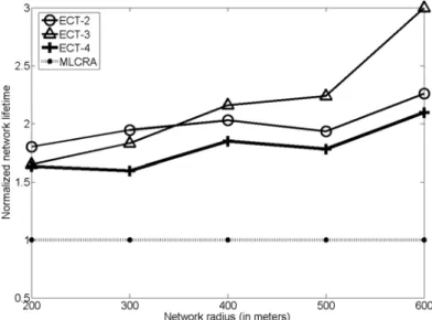
Fig. 7. Normalized network lifetime comparison between ECT and MLCRA

Fig. 6 compares the proposed ECT with the MLCRA protocol. We regard the ECT scheme with k-corona model as ECT-k. It shows that ECT-2 (2-corona model), ECT-3 (3-corona model) and ECT-4 (4-corona model) exceed MLCRA protocol for the network lifetime. This is due to the fact that, the ECT using nearly balanced energy analysis scheme to determine

(12)

cluster radius and transmission ranges in each corona. Fig. 7 compares the proposed ECT with the MLCRA protocol in terms of normalized network lifetime.

To evaluate the impact for 2-corona model (ECT-2), 3-corona model (ECT-3) and 4-corona model (ECT-4), we first measure the network lifetime of ECT scheme versus the network radius ranges from 200m to 600m. T is fixed at 20 percent (T is the threshold of CH power, as mentioned in Section 5.3). From Fig. 8, we can clearly observe that ECT-2 gets better network lifetime when the network radius is 200m and 300m; ECT-3 is recommended when the network radius exceeds 400m. In fact, the same trends hold for T=15% and T=10%. Furthermore, the network lifetime has a decreasing trend as the network radius increases. This is because when network radius increases, transmission distances are increased for each sensor node. Hence, the network lifetime is decreased.

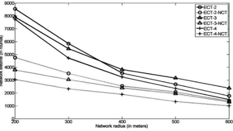
Fig. 9 shows the network lifetime of ECT scheme and the ECT-NCT (Non Cross Transmissions) scheme. The difference between the ECT scheme and ECT-NCT scheme is that the ECT does cross-corona data transmissions (CT) while ECT-NCT scheme does not. It is worth mentioning that the ECT-2 scheme has longer network lifetime than the ECT-2-NCT scheme when the network operation is terminated. Likewise, ECT-3 scheme and ECT-4 schemes improve the network lifetime when compared with the ECT-3-NCT scheme and the ECT-4-NCT scheme, respectively. It also indicates that cross-corona data transmissions have benefits.

Fig. 8. Network lifetime comparison between ECT-2, ECT-3 and ECT-4

(13)

6.2 Residual Energy of Each Sensor Node

To evaluate our ECT scheme in terms of residual energy (RE), we also compare it to the MLCRA scheme. We only choose the ECT-3 scheme since simulation results show it has good performance (compared to ECT-2 and ECT-4). The network radius is set to 500m.

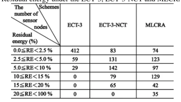
For ECT-3, most of the sensor nodes nearly use up their energy when the network operation ends as shown in Table 2. As a matter of fact, the residual energy of most sensor nodes is below 2.34×10-2 joule when utilizing our ECT-3 scheme. By comparison, we can see that the residual energy improvement of ECT-3 scheme compared to the ECT-3-NCT scheme.

MLCRA algorithm follows the CH rotations used by the LEACH-DCHS [15]. However, MLCRA does not guarantee the energy depletion can be consumed in the well-balanced status. From Table 2, we can see that the ECT-3 scheme is more energy efficiency than the MLCRA scheme.

Table 2. Residual energy under the ECT-3, ECT-3-NCT and MLCRA schemes

6.3 Total Number of CH Rotations

As mentioned earlier in Section 5.3, many traditional clustering algorithms frequently rotate the role of CH so that the loads can be shared among all sensor nodes. However, periodical CH rotations increase considerable overheads. Therefore, we need to reduce the total number of CH rotations if possible.

Table 3 shows the total number of CH rotations for ECT-2, ECT-3, ECT-4 and MLCRA. We observe that, as threshold T increases, the total number of CH rotations also increases. This is because larger threshold T triggers the CH rotations earlier. Furthermore, CH rotations of ECT-2 are less than that of the ECT-3 and ECT-4 schemes (for T of 10, 15 and 20 percent). Specifically, CH rotations of ECT-2 can be reduced by 14.8 percent (compared to ECT-3) and 17.4 percent (compared to ECT-4) when the threshold T is set to 10 percent.

As to the MLCRA algorithm, it frequently rotates the role of CHs to share the loads among all sensor nodes. As a result, its number of CH rotations is much larger.

(14)

7. Conclusions

In this paper, we proposed a novel energy balanced clustering mechanism ECT to extend the network lifetime in corona-based WSNs. The main idea is to divide network into varies cluster radiuses based on the energy consumption among CHs for each corona. Simulation results show that the ECT protocol can efficiently improve network lifetime, achieve energy efficiency and reduce CH rotations compared to the MLCRA protocol.

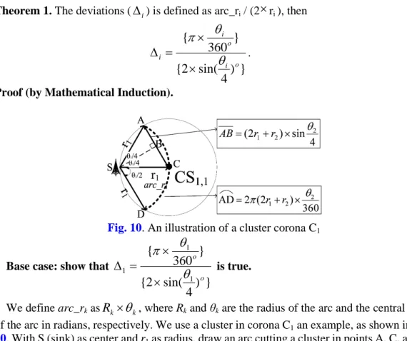
Appendix

Theorem 1. The deviations (

∆

_i) is defined as arc_ri / (2

×

ri ), then

}

)

4 sin(

2 {

}

360 {

o i o i i

θ

π

×

=

∆

. (1)

Proof (by Mathematical Induction).

Fig. 10. An illustration of a cluster corona C1

Base case: show that

}

)

4 sin(

2 {

}

360 {

1 1 1 o o

θ

π

×

=

∆

is true.

We define arc_rk as

R

_k

×

θ

_k, where Rk and θk are the radius of the arc and the central angle

of the arc in radians, respectively. We use a cluster in corona C1 an example, as shown in Fig. 10. With S (sink) as center and r1 as radius, draw an arc cutting a cluster in points A, C, and D. Without loss of generality, we let ∠ASD =

θ

₁. Since ─_{SA =}_{SC =}─ _{SD = R}─ 1 = r1, then arc_r1

=

⌒

_ACD=

R

1

×

θ

1= r o 360 ) ( 2 1 1

θ

π

× . Because ─_{SC is a bisector of ∠ASD, ∠ASC = ∠CSD} =

2

1

θ

. △ASC is an isosceles triangle since ─_SA=_{SC. Let the midpoint of}─ _{AC be B. Since B lies}─ on the perpendicular bisector of ─_{AC, therefore}_AB=─ _{BC and ∠ASB =∠BSC =}─

4 1

θ

. Then 2×r1 = 4 × ─_AB= 4 sin ) ( 4 1 1

θ

× × r . Finally, we have

(15)

1 1 1

2 _

r

arc

×

=

∆

=

}

)

4 sin(

)

(

4 {

}

360 )

(

2 {

1 1 1 1 o o

r

θ

π

×

}

)

4 sin(

2 {

}

360 {

1 1 o o

θ

π

×

=

.

Hence, the equality holds when i = 1.

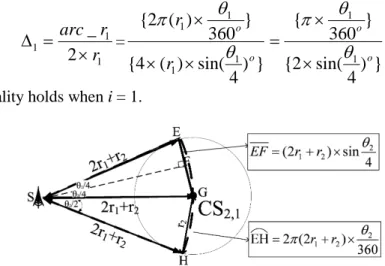
Fig. 11. An illustration of a cluster corona C2

Base case: show that

}

)

4 sin(

2 {

}

360 {

2 2 2 o o

θ

π

×

=

∆

is true.

We use a cluster in corona C2 an example, as shown in Fig. 11. Without loss of generality, we let ∠ ESH =

θ

₂ . Since ─_{SE =} _{SG =}─ _{SH = R}─ 2 = 2r1+r2, then arc_r2 =

⌒

EGH =

2 2

×

θ

R

=

r

_o

360 )

2 (

2

2 2 1

θ

π

+

×

. Similar to

∆

₁, the detailed description in this part can be omitted. Then 2×r2= 4× ─EF = 4 sin ) 2 ( 4 2 2 1

θ

× + × r r . Finally, we have 2 2 2

2 _

r

arc

×

=

∆

=

}

)

4 sin(

)

2 (

4 {

}

360 )

2 (

2 {

2 2 1 2 2 1 o o

r

θ

π

×

+

×

+

}

)

4 sin(

2 {

}

360 {

2 2 o o

θ

π

×

=

.

As a result, the equality holds when i = 2.

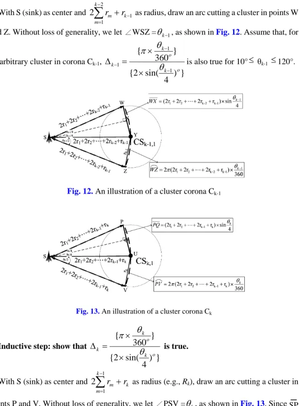
Inductive hypothesis: assume that

}

)

4 sin(

2 {

}

360 {

1 1 1 o k o k k − − −

×

=

∆

_θ

θ

π

is true.

(16)

With S (sink) as center and 1 2 1 2 ₋ − = +

∑

k k m m r

r as radius, draw an arc cutting a cluster in points W and Z. Without loss of generality, we let ∠WSZ =

θ

k−1, as shown in Fig. 12. Assume that, for

an arbitrary cluster in corona Ck-1,

}

)

4 sin(

2 {

}

360 {

1 1 1 o k o k k − − −

×

=

∆

_θ

θ

π

is also true for 10°

≤

θk-1

≤

120°.

Fig. 12. An illustration of a cluster corona Ck-1

Fig. 13. An illustration of a cluster corona Ck

Inductive step: show that

}

)

4 sin(

2 {

}

360 {

o k o k k

θ

π

×

=

∆

is true.

With S (sink) as center and _k

k m m r r +

∑

− = 1 1

2 as radius (e.g., Rk), draw an arc cutting a cluster in

points P and V. Without loss of generality, we let ∠PSV =

θ

_k, as shown in Fig. 13. Since ─_SP

= ─_{SU =} _{SV =}─ _k k m m r r +

∑

− = 1 1

2 , then arc_rk =

⌒

PUV =

R

k

×

θ

k = o

k k k m m r r 360 ) 2 ( 2 1 1

θ

π

∑

− + × = .

(17)

Because ─_{SU is a bisector of ∠PSV, ∠PSU =∠USV =}

2

k

θ

. △PSU is an isosceles triangle since ─_{SP =}_{SU. Let the midpoint of}─ _{PU be Q. Since Q lies on the perpendicular bisector of}─ _PU─ , therefore ─_PQ=_{QU and ∠PSQ =∠QSU=}─

4 k

θ

. Then 2×rk= 4× ─PQ= 4 sin ) 2 ( 4 1 1 k k m k m r r + ×

θ

×

∑

− = . Hence, we get k k k

r

arc

×

=

∆

2 _

=

}

)

4 sin(

)

2 (

4 {

}

360 )

2 (

2 {

1 1 1 1 o k k k m m o k k k m m

r

θ

π

×

+

×

+

∑

− = − =

}

)

4 sin(

2 {

}

360 {

o k o k

θ

π

×

=

.

This completes the proof of the theorem.

References

[1] M. V. MICEA, A. STANCOVICI, D. CHICIUDEAN and C. FILOTE, “Indoor Inter-Robot Distance Measurement in Collaborative Systems,” Advances in Electrical and Computer

Engineering, Vol. 10, pp. 21–26, 2010. Article (CrossRef Link)

[2] M.L. Filograno, P. Corredera Guillen, A. Rodriguez-Barrios, S. Martin-Lopez, M. Rodriguez-Plaza, A. Andres-Alguacil, and M. Gonzalez-Herraez, “Real-Time Monitoring of Railway Traffic Using Fiber Bragg Grating Sensors,” IEEE Sensors Journal, Vol. 12, pp. 85–92, 2012. Article (CrossRef Link)

[3] J. Li, Q.S. Jia, X. Guan, and X. Chen, “Tracking a moving object via a sensor network with a partial information broadcasting scheme,” Information Sciences, Vol. 181, pp. 4733–4753, 2011.

Article (CrossRef Link)

[4] T. Kwon, and J. Hong, “Secure and Efficient Broadcast Authentication in Wireless Sensor Networks,” IEEE Transaction on Computers, Vol. 59, pp. 1120–1133, 2010.

[5] I. FERNÁNDEZ, A. ASENSIO, I. GUTIÉRREZ, J. GARCÍA, I. REBOLLO and J. d. NO, “Study of the communication distance of a MEMS Pressure Sensor Integrated in a RFID Passive Tag,” Advances in Electrical and Computer Engineering, Vol. 12, pp. 15–18, 2012.

[6] S.J Jung, T.H. Kwon, and W.Y. Chung, “A new approach to design ambient sensor network for real time healthcare monitoring system,” IEEE Sensors, pp. 576–580, 2009.

[7] E.I. Gokce, A.K. Shrivastava, J.J. Cho, and Y. Ding, “Decision Fusion from Heterogeneous Sensors in Surveillance Sensor Systems,” IEEE Transaction Automation Science and Engineering, Vol. 8, pp. 228–233, 2011. Article (CrossRef Link)

[8] Y. Park, Y. Park, and S. Moon, “Privacy-preserving ID-based key agreement protocols for cluster-based MANETs,” Int. J. of Ad Hoc and Ubiquitous Computing, Vol. 14, pp. 78–89, 2013.

[9] L. Guo, B. Wang, C. Gao, W. Xiong, and H. Gao, “The Comprehensive Energy-Routing Protocol Based on Distributed Cluster Optimization in Wireless Sensor Networks,” Sensor Lett., Vol. 11, pp. 966-973, 2013. Article (CrossRef Link)

[10] A.S. Poornima, and B.B. Amberker, “PERSEN: power-efficient logical ring based key management for clustered sensor networks,” Int. J. of Sensor Networks, Vol. 10, pp. 94–103, 2011.

[11] Sangwook Kang, Sangbin Lee, Saeyoung Ahn and Sunshin An, “Energy Efficient Topology Control based on Sociological Cluster in Wireless Sensor Networks,” KSII Transactions on

(18)

Internet and Information Systems, Vol. 6, pp. 341–360, 2012. Article (CrossRef Link)

[12] B. Elbhiri, R. Saadane and D. Aboutajdine, “Stochastic and Equitable Distributed Energy-Efficient Clustering (SEDEEC) for heterogeneous wireless sensor networks,” Int. J. of Ad Hoc and

Ubiquitous Computing, Vol. 7, pp. 4–11, 2013. Article (CrossRef Link)

[13] J. Li, and P. Mohapatra, “Analytical modeling and mitigation techniques for the energy hole problems in sensor networks,” Pervasive and Mobile Computing, Vol. 3, pp. 233–254, 2007.

[14] W.R. Heinzelman, A. Chandrakasan, and H. Balakrishnan, “Energy-Efficient Communication Protocol for Wireless Microsensor Networks,” in Proc.of Hawaii Int. Conf. on System Sciences

(HICSS), pp. 1–10, 2000. Article (CrossRef Link)

[15] Y. Liu, J. Gao, Y. Jia, and L. Zhu, “A Cluster Maintenance Algorithm Based on LEACH-DCHS Protocol,” in Proc of IEEE Int. Conf. Networking, Architecture, and Storage, pp. 165–166, 2008.

[16] M. YE, C. LI, G. CHEN, and J. WU, “An energy efficient clustering scheme in wireless sensor networks,” Int. J. Ad Hoc and Sensor Wireless Networks, Vol. 3, pp. 99–119, 2007.

[17] J. Lian, K. Naik, and G. Agnew, “Data capacity improvement of wireless sensor networks using non-uniform sensor distribution,” Int. J. Distributed Sensor Networks, Vol. 2, pp. 121–145, 2006.

[18] Y. Liu, N. Xiong, Y. Zhao, A.V. Vasilakos, J. Gao, and Y. Jia, “Multi-layer clustering routing algorithm for wireless vehicular sensor networks,” IET Commun., Vol. 4, pp. 810–816, 2010.

[19] W.R. Heinzelman, A. Chandrakasan, and H. Balakrishnan, “An application-Specific Protocol Architecture for Wireless Microsensor Networks,” IEEE Transaction Wireless Commun., Vol. 1, pp. 660–670, 2002. Article (CrossRef Link)

[20] Wolfram Mathematica 7.0. http://www.wolfram.com/mathematica/

[21] H. Shen, “Finding the k Most Vital Edges with Respect to Minimum Spanning Tree,” in Proc.of IEEE National on Aerospace and Electronics Conf. (NAECON), Vol. 1, pp. 255–262, 1997.

(19)

Wei Kuang Laireceived a BS degree in Electrical Engineering from National Taiwan University, Taiwan in 1984 and a Ph.D. degree in Electrical Engineering from Purdue University in 1992. He is a professor in Department of Computer Science and Engineering, National Sun Yat-sen University, Taiwan. His research interests are in wireless networks and high-speed networks. He was a visiting fellow at Electrical Engineering of Princeton University from August 2010 to June 2011, where he was involved in applying machine learning for clustering and routing of network nodes.

Chung-Shuo Fan received the M.S. degree in Computer Science and Information Engineering from National Changhua University of Education, Changhua, Taiwan, in 2007, and the Ph.D. degree in Computer Science and Engineering, National Sun Yat-Sen University, Kaohsiung, Taiwan, in 2012. Currently, he is a postdoctoral fellow in Department of Computer Science, National Chiao Tung University, Taiwan. His research interests include wireless sensor networks and vehicular ad-hoc networks.

Chin-Shiuh Shieh received the M.S. degree in electrical engineering from the National Taiwan University, Taipei, Taiwan, in 1991 and the Ph.D. degree in computer science and engineering from the National Sun Yat-Sen University, Kaohsiung, Taiwan in 2009. In August 1991, he joined the faculty of the Department of Electronic Engineering, National Kaohsiung University of Applied Sciences, Kaohsiung, where he is currently an Associate Professor. His research interests include wireless networks and handover techniques.