IEEE 802.15.3c 無線個人區域網路之單載波區塊傳輸基頻接收機的設計與模擬

國 立 交 通 大 學

電信工程學系

碩 士 論 文

IEEE 802.15.3c 無線個人區域網路之單載波

區塊傳輸基頻接收機的設計與模擬

Design and Simulation of the Baseband Receiver for Single

Carrier Block Transmission in IEEE 802.15.3c

Wireless Personal Area Network

研究生：汪奕廷

指導教授：黃家齊 博士

IEEE 802.15.3c 無線個人區域網路之單載波

區塊傳輸基頻接收機的設計與模擬

Design and Simulation of the Baseband Receiver for Single Carrier Block

Transmission in IEEE 802.15.3c Wireless Personal Area Network

研 究 生：汪奕廷 Student：Yi-Ting Wang

指導教授：黃家齊 博士 Advisor：Dr. Chia-Chi Huang

國 立 交 通 大 學

電信工程學系

碩 士 論 文

A Thesis

Submitted to Department of Communication Engineering College of Electrical and Computer Engineering

National Chiao Tung University in partial Fulfillment of the Requirements

for the Degree of Master of Science

in

Communication Engineering June 2009

Hsinchu, Taiwan, Republic of China

IEEE 802.15.3c 無線個人區域網路之單載波

區塊傳輸基頻接收機的設計與模擬

學生：汪奕廷

指導教授：黃家齊博士

國立交通大學電信工程學系 碩士班

摘

要

為了提供室內高速個人區域網路的需求，IEEE 802.15.3c 的標準被制定

出來。它兼採單載波區塊傳輸和正交頻分多工兩種調變方式，操作在 60GHz

免認證頻段，所提供的傳輸速率為 1 Gbps 以上。這篇論文將依據 IEEE

802.15.3c 標準內單載波區塊傳輸所規定的封包格式設計其基頻接收機架

構，其中包含符元時序估計、通道估計、頻域等化器、及資料檢測等部分。

每個部分將針對其運作原理及演算法做詳細的介紹，在每個部分中盡可能

在性能表現與運算複雜度間取一平衡點。為了驗證接收機的效能，我們進

行各種電腦模擬，特別在資料檢測的部分我們會提出各種方法來提升接收

機在位元錯誤率上的表現，並計算其運算複雜度作為參考。最後我們提出

結論與未來的研究方向。

Design and Simulation of the Baseband Receiver for Single Carrier Block

Transmission in IEEE 802.15.3c Wireless Personal Area Network

Student：Yi-Ting Wang

Advisors：Dr. Chia-Chi Huang

Department of

Communication Engineering

National Chiao Tung University

ABSTRACT

The IEEE 802.15.3c WPAN standard was defined in order to support the demand of high data rate indoor transmission. It adopts SCBT and OFDM modulations and operates at 60 GHz unlicensed band. Hope to provide data rates more than 1 Gbps. In this thesis, we propose an IEEE 802.15.3c SCBT baseband receiver architecture according to its specified frame format. The receiver includes symbol timing estimation, channel estimation, frequency domain equalization, and data detection. We will describe the operation principles and the algorithms of each block in details. And we try to make a tradeoff between system performance and computation complexity. In order to verify the performance of the receiver, computer simulations are conducted under different conditions. Especially in data detection part, we propose several methods to enhance the performance of the receiver in BER, and we will calculate the complexity of computation as references as well. Finally, we draw conclusions and comments on possible future research directions.

誌 謝

首先要感謝我的指導老師黃家齊教授在這兩年來的指導，提供了良好的

學習與研究環境使我得以專注在學業上並順利完成這兩年的學業。另外特

別感謝古孟霖學長總是不厭其煩的與我討論我的研究，並提供了許多經驗

幫我解決了許多問題，使我收穫良多。並感謝口試招集人吳文榕教授、委

員陳紹基教授與高銘盛教授，提供許多寶貴的意見使得我的論文能更為完

整。

接著感謝我親愛的家人們從小到大對我的栽培與照顧，在外念書的期

間雖然總是聚少離多，但他們依舊願意給我溫暖與後盾在背後支持著、鼓

勵著我，讓我能夠心無旁騖的完成自身的學業。

感謝同為碩二的同學們冠群、丁丁、王森和小顗這兩年來的照顧與陪

伴，彼此之間的幫忙扶持讓上課與研究都更加的有趣與踏實。另外也感謝

碩班的學長姐，阿威、建勳、文娟與思潔還有學弟妹小馬、煒翰、詠仁與

佳儀，雖然相處的時間不多，但這一切都因為有你們而更加的充實。

另外感謝 NTL 實驗室的朋友們，雖然是在偶然的情況下認識，但你們

總是願意把我當成實驗室的一分子關心著我，讓我倍感溫暖。還要感謝一

起打球的朋友們，歪歪、黑人、Sony、忠傑、Sky 等人，還有從大學起就一

路照顧著我的紹峰學長，與你們打球的時間和比賽的過程都是我相當珍貴

的回憶。

最後我要感謝我的女朋友簡家齊，在交往的過程中總是體貼著我，給

我很多精神上的支持與鼓勵，讓我更有勇氣並且積極的面對一切的困難與

挑戰。

iv

Contents

Chapter 1 Introduction ……….…..1

1.1 IEEE 802.15.3c WPAN ……….…...1

1.2 Challenges ...……….2

1.3 About the thesis …...……….3

Chapter 2 Single carrier (SC) system (vs. OFDM) …...……….4

2.1 Compare with OFDM ...………...4

2.2 Single Carrier Block Transmission (SCBT) ...……….5

Chapter 3 IEEE 802.15.3c WPAN PHY standard ……….9

3.1 Channelization ……….9

3.2 Frame Format …...………..10

3.3 PLCP Preamble ...………...12

Chapter 4 IEEE 802.15.3c single carrier receiver structure ……….14

4.1 Block diagram ...……….14

4.2 Synchronization ...………..16

4.3 Channel estimation ...……….……….22

4.3.1 Golay complementary code ...……….……….22

4.3.2 Channel estimation scheme ...………..……….23

4.4 Equalization ...………28

4.5 Data detection ...……….32

4.5.1 Gibbs sampler (GS) ...………...33

4.5.1.1 Markov Chain Monte Carlo method ...……….33

4.5.1.2 Gibbs sampler ...………...35

4.5.2 Multi-path interference cancellation (MPIC) .………..39

v

Chapter 5 Simulation results ...……….49

5.1 Simulation results of synchronization ...……….49

5.2 Simulation results of channel estimation ...………53

5.3 Simulation results of frequency domain equalization ...……….60

5.4 Simulation results of data detection ………...62

Chapter 6 Conclusions ...………..74

Appendix …………...………..76

vi

List of Tables

Table 3.1 Parameters of IEEE 802.15.3c channel plan (full rate) ………..……….9

Table 3.2 Parameters of IEEE 802.15.3c channel plan (half rate) ………..9

Table 3.3 IEEE 802.15.3c frame format parameters ……….12

Table 4.1 Synchronization algorithm ………21

Table 4.2 Channel estimation method ………...26

Table 4.3 Modified channel estimation method ………27

Table 4.4 General Gibbs Sampler algorithm ………35

Table 4.5 Gibbs Sampler algorithm in SCBT data detection ………37

Table 4.6 MPIC detector method in SCBT data detection ………...42

Table 4.7 PDA algorithm ………..…46

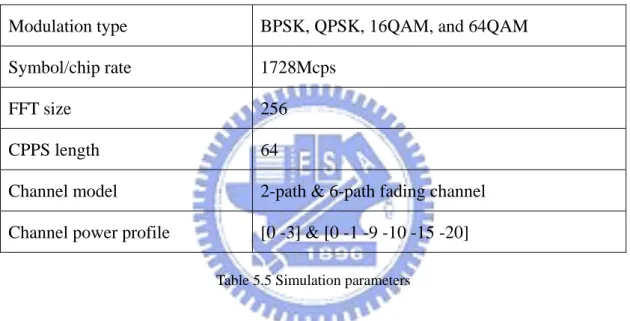
Table 4.8 Simulation parameters ………..47

Table 5.1 Parameters for synchronization in 2-path fading channel ………...…49

Table 5.2 Probability of tracking on each path as the first path for different γ ……….51

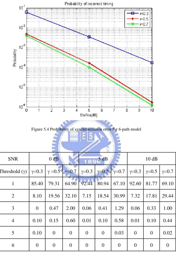
Table 5.3 Parameters for synchronization in 6-path fading channel …………...……51

Table 5.4 Probability of tracking on each path as the first path for different γ …….…52

Table 5.5 Simulation parameters ………..…53

Table 5.6 Patterns of error number after each iteration in figure 5.34 ………..…71

vii

List of Figures

Figure 2.1 OFDM and SCBT Tx ………...………….………6

Figure 2.2 OFDM and SCBT Rx ………...……….………6

Figure 2.3 Performances for SCBT and OFDM system in 2-path channel ...…………7

Figure 2.4 Performances for SCBT and OFDM system in 6-path channel ...…………8

Figure 3.1 IEEE 802.15.3c channel plan (full rate) ...……….………9

Figure 3.2 IEEE 802.15.3c channel plan (half rate) ...……….9

Figure 3.3 IEEE 802.15.3c Frame Format …………...……….11

Figure 3.4 Structure of Frame Payload ...………..11

Figure 3.5 IEEE 802.15.3c PHY preamble structure ...……….13

Figure 4.1 SCBT baseband receiver structure ...………...14

Figure 4.2 IEEE 802.15.3c SCBT synchronization sequence ...………16

Figure 4.3 Auto-correlation of Golay code with 128 chips ..………17

Figure 4.4 An example of received SYNC sequence in two path channel ...…………17

Figure 4.5 2 paths channel impulse responses ...………...18

Figure 4.6a Output sequence of matched filter ...………..19

Figure 4.6b Mapping the CIR on output of matched filter ...………19

Figure 4.7 Flow chart of synchronization algorithm ……….20

Figure 4.8 Auto-correlation of complementary codes with length 256 ..………..23

Figure 4.9 Structure of IEEE 802.15.3c SCBT CE sequence ...………24

Figure 4.10 An Example of channel estimation scheme …..……….24

Figure 4.11 Original channel impulse responses …...………...25

Figure 4.12 Estimated channel impulse responses with noise ...………...26

Figure 4.13 The block diagram of FDE ...……….29

viii

Figure 4.14 The block diagram of our Gibbs Sampler detector ………38

Figure 4.15 Received data signal over multipath channel ...……….39

Figure 4.16 The block diagram of our MPIC detector ………..41

Figure 4.18 Performances of SD and PDA for FFT size=32 ...……….………47

Figure 4.19 Performances of SD and PDA for FFT size=64 ...……….………48

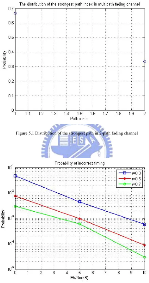
Figure 5.1 Distribution of the strongest path in 2-path fading channel ...…………..50

Figure 5.2 Probability of synchronization error for 2-path model ……….50

Figure 5.3 Distribution of the strongest path in 6-path fading channel ...…………..51

Figure 5.4 Probability of synchronization error for 6-path model ...………..52

Figure 5.5 Normalize mean square error of CIRs with different γ...………….……..54

Figure 5.6 Normalize mean square error of NP with different γ ...………….…….…55

Figure 5.7 Performance of estimated CSI with different γ in BER (BPSK) ...…...55

Figure 5.8 Performance of estimated CSI with different γ in BER (QPSK) ...………56

Figure 5.9 Performance of estimated CSI with different γ in BER (16QAM) ..…….56

Figure 5.10 Performance of estimated CSI with different γ in BER (64QAM) ..…….57

Figure 5.11 Normalize mean square error of CIRs with different γ ..………….……..57

Figure 5.12 Normalize mean square error of NP with different γ ..…….……….58

Figure 5.13 Performance of estimated CSI with different γ in BER (BPSK) ..………58

Figure 5.14 Performance of estimated CSI with different γ in BER (QPSK) ..………59

Figure 5.15 Performance of estimated CSI with different γ in BER (16QAM) ..…….59

Figure 5.16 Performance of estimated CSI with different γ in BER (64QAM) ..…….60

Figure 5.17 BER for FDE with different modulations in 2-path channel ..………….61

Figure 5.18 BER for FDE with different modulations in 6-path channel ..………….61

Figure 5.19 GS detector with different iteration numbers (BPSK) ..………...….62

ix

Figure 5.21 GS detector with different iteration numbers (QPSK) ...………...63

Figure 5.22 MPIC detector with different iteration numbers (QPSK) ..………...64

Figure 5.23 GS detector with different iteration numbers (16QAM) ..………64

Figure 5.24 MPIC detector with different iteration numbers (16QAM) ..………65

Figure 5.25 GS detector with different iteration numbers (64QAM) ..………65

Figure 5.26 MPIC detector with different iteration numbers (64QAM) ..………66

Figure 5.27 GS detector with different iteration numbers (BPSK) ..………67

Figure 5.28 MPIC detector with different iteration numbers (BPSK) ..………...68

Figure 5.29 GS detector with different iteration numbers (QPSK) ..………...68

Figure 5.30 MPIC detector with different iteration numbers (QPSK) ..………...69

Figure 5.31 GS detector with different iteration numbers (16QAM) ..………69

Figure 5.32 MPIC detector with different iteration numbers (16QAM) ..………70

Figure 5.33 GS detector with different iteration numbers (64QAM) ..………70

Figure 5.34 MPIC detector with different iteration numbers (64QAM) ..………71

Figure 5.35 Different data detection methods (BPSK) ..…….……….73

1 

Chapter 1 Introduction

To respond the demands for very high data rates indoor wireless communication such as

uncompressed high definition video streaming, flash file downloading and so on, many

applications for high speed and short range transmission are being standardized. For example,

IEEE 802.11 very high throughput (VHT) and wireless HD are proposed. IEEE 802.15.3c

wireless personal area network (WPAN) is one of them to satisfy such requirements. In this

chapter, we will briefly describe the situation of this standard including potential,

requirements, and challenges. And we will introduce organization of this thesis at the end of

this chapter as well.

1.1 IEEE 802.15.3c WPAN

The millimeter-wave 60 GHz WPAN is being standardized by the IEEE 802.15

Alternative PHY Task Group 3c (IEEE 802.15.3c). This emerging IEEE 802.15.3c standard

targets the data rates of multi-giga bits per second (multi-Gbps) for short range around 5 to 10

meters indoor applications [1].

The realization of such high speed wireless transmission has long been obstructed mainly

by two critical factors: one is the lack of spectrum which is wide enough and the other is the

high cost of high frequency circuits and device. Recently, the substantial unlicensed spectrum

2 

technology drives the cost of 60 GHz circuits and devices much lower than in the past.

There are two kinds of systems in this standard. One is the OFDM mode, and the other is

the single carrier (SC) mode. Common mode which enables the IEEE 802.15.3c devices

having different PHYs (SC and OFDM) to communicate with each other, and it is therefore a

key technique for standardization to realize flexible systems with easy expandability from SC

to OFDM or other SCs and vice versa. After comparing SC with OFDM, we found that SC

system is more suitable in application in IEEE 802.15.3c WPAN system. We focus on SC

system receiver design only in this paper.

1.2 Challenges

Despite its huge potentials to achieve Gbps data rate, 60 GHz system has a number of

technical challenges and many open issues to be solved before its full deployment. One of

them is channel propagation issue, which causes significantly higher path loss at 60 GHz than

those at lower frequencies. According to this issue, the propagation range of 60 GHz must be

shorter, usually in 5 to 10 meters, than other system. Although the price of such high speed

circuit is much lower than in the past, the peak to average power ratio (PAPR) issue still

remains in transceiver design. Another important issue is the computation complexity of the

system. To achieve such high data rates, the design of the system structures and the methods

3 

1.3 About the thesis

This paper is organized as following. Chapter 2 compares the SC and OFDM systems.

Then we will introduce the advantages and remaining issues of each system. In chapter 3, we

will give a simple introduction of IEEE 802.15.3c standard draft 3. We focus on the PHY

layer specification, and base on this standard to develop our baseband receiver. The baseband

receiver that we proposed will be shown in chapter 4. The receiver contains synchronization,

channel estimation, equalization, and data detection parts. The simulation results of each part

in SC receiver will be shown in chapter 5. Finally, we will make our conclusions and future

4 

Chapter 2 Single carrier (SC) system (vs. OFDM)

In this chapter, we will introduce the SC system. And we will make a comparison

between SC and OFDM systems. Some open issues of OFDM system such as PAPR issue,

effect of carrier frequency offset (CFO), and so on will be mentioned at later of this chapter.

According to the requirements of our system, SC system outperforms OFDM system. So we

choose the SC system as our proposed receiver structure for IEEE 802.15.3c WPAN. At last,

we will simply introduce the single carrier block transmission (SCBT) system in the end of

this chapter.

2.1 Compare with OFDM

Orthogonal frequency division multiplexing (OFDM) has already been included in

digital audio/video broadcasting (DAB/DVB) standard in Europe, and has been successfully

applied to high-speed digital subscriber line (DSL) modems in the United States.

To annihilate inter-block interference (IBI) between successive inverse fast Fourier

transform (IFFT) processed blocks, a cyclic prefix (CP) of length no less than the channel

order is inserted per transmitted block. Discard the CP at the receiver not only suppresser IBI,

but also converts the linear channel convolution into circular convolution, which means after

converted by FFT the channel frequency will be one tap for each sub-carrier. By

5 

inter-symbol interference (ISI) channel into parallel ISI-free sub-channels with gains equal to

channel frequency response values on FFT grid.

Although OFDM enables simple equalization, it introduces the following three

well-known problems: one is the PAPR of the transmitted signal power is large, necessitating

power back off. SC modulation uses a single carrier, instead of the many typically used in

OFDM, so the PAPR is smaller than multi-carrier systems. The other is that OFDM system is

very sensitive to transmit-receive oscillator mismatch which cause CFO. The last problem is

that the uncoded OFDM system does not enable the available multipath diversity, as described

in [2].

Consortium of Millimeter wave Practical Applications (CoMPA) has been established to

promote single carrier (SC) modulation for the future WPAN system. This is because SC

modulation has several advantages in realizing low-cost and low-power consumption devices

over multi-carrier modulation especially in short range communications environment [3].

2.2 Single Carrier Block Transmission (SCBT)

In order to reduce the complexity of equalization, we copy the last part of each single

carrier data block as CP which is the same operation as OFDM time domain signals. Then we

can equalize the ISI caused by multi-path effect by one-tap equalizer on each subcarrier in

Moreover, from figure 2.1 and figure 2.2, we can easily found that the difference between

SCBT and OFDM systems is only the position of IFFT operation, but the overall system

complexities remain the same.

OFDM Tx

SCBT Tx

Figure 2.1 OFDM and SCBT Tx OFDM Rx

SCBT Rx

Figure 2.2 OFDM and SCBT Rx

Compare to OFDM system, SCBT system with frequency domain equalization has

similar performance, efficiency, and low signal processing complexity advantages as OFDM.

SCBT system also has several advantages. SCBT system reduces PAPR requirement. This in

turn means that the power amplifier of the SC transmitter requires a smaller linear range to

support the given average power. This enables the use of a cheaper power amplifier than a

comparable OFDM system, as mentioned in [4]. And in addition are less sensitive than

OFDM to radio frequency (RF) impairments such as CFO which caused by the mismatch of

oscillators in transmitter and receiver. According to these attractive features, we choose the

SCBT system as our 60 GHz receiver.

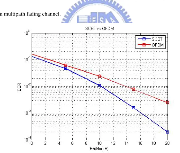
In figure 2.3 and 2.4, we can easily find the performances for SCBT system are much

better than OFDM system in BER comparison. Furthermore, the BER curves for OFDM are

almost the same. That because the signals in OFDM are carried by frequency, and it can’t

obtain any diversity from multipath fading channel. The performances for SCBT are quite

different according to the different path numbers. More path number gets better performance.

Different from OFDM system, the signals in SCBT system can gain diversity in time domain

from multipath fading channel.

Figure 2.3 Performances for SCBT and OFDM system in 2-path channel

Figure 2.4 Performances for SCBT and OFDM system in 6-path channel

Chapter 3 IEEE 802.15.3c WPAN PHY standard

In this chapter, we will introduce IEEE 802.15.3c physical layer specification. Include

channelization in 60 GHz unlicensed band, frame format which contains the structure of

headers, preambles, and data symbols, and the physical (PHY) layer convergence protocol

(PLCP) preamble which contains the information for synchronization (SYNC) and channel

estimation (CE).

3.1 Channelization

IEEE 802.15.3c WPAN is operated at 60GHz unlicensed band. Divide this frequency

band into four independent channels. Figure 3.1 and 3.2 show the channel plans of full and

half rate transmission. The detail parameters of these four channels are listed in table 3.1 and

3.2 which are full rate and half rate, respectively.

(GHz) f

58.320

60.480

62.640

64.800

Figure 3.1 IEEE 802.15.3c channel plan (full rate)

(GHz) f

58.320

60.480

62.640

64.800

10    Channel number Low freq. (GHz) Center freq. (GHz) High freq. (GHz) Nyquist BW (MHz) Roll off factor CH#1 57.240 58.320 59.400 1728 0.25 CH#2 59.400 60.480 61.560 1728 0.25 CH#3 61.560 62.640 63.720 1728 0.25 CH#4 63.720 64.800 65.880 1728 0.25

Table 3.1 Parameters of IEEE 802.15.3c channel plan (full rate)

Channel number Low freq. (GHz) Center freq. (GHz) High freq. (GHz) Nyquist BW (MHz) Roll off factor CH#1 57.240 58.320 59.400 1728 0.25 CH#2 59.400 60.480 61.560 1728 0.25 CH#3 61.560 62.640 63.720 1728 0.25 CH#4 63.720 64.800 65.880 1728 0.25

Table 3.2 Parameters of IEEE 802.15.3c channel plan (half rate)

3.2 Frame Format

Frame format that includes a preamble providing sufficient robustness against wireless

the preamble is Golay code, which realizes a reduced SYNC circuit, and which can also be

shared with the channel estimator.

Figure 3.3 shows the proposed frame format for IEEE 802.15.3c standardization. The

frame format consists of a PHY preamble, frame header, and frame payload including pilot

channel estimation sequence (PCES) and data slot. Frame header contains PHY and MAC

headers which include the information that used in PHY and MAC layers. The PHY preamble

which is also named PLCP preamble will be introduced in detail in next section.

PHY Preamble (long, short, or middle) Frame Header Frame Payload

Figure 3.3 IEEE 802.15.3c Frame Format

The structure of frame payload is shown in figure 3.4. A data slot consists of cyclic

prefix pilot symbols (CPPS) with different length and SCBT data blocks with two sizes, 256

and 512. The most important role of CPPS is used as CP for frequency domain equalization

which is used for compensating the multi-path effect. The PCES here is used for timing

tracking, CFO compensation, and more accurate channel estimation. More parameters of

IEEE 802.15.3c frame format are listed in table 3.3.

M

a

a

a

a

Figure 3.4 Structure of Frame Payload 11 

12 

Data block size PCES length PCES period CPPS length

256 (mandatory) 768 8192, 16384, or 32768 16, 32, or 64

512 (option) 1536 8192, 16384, or 32768 32, 64, 96, or 128

Table 3.3 IEEE 802.15.3c frame format parameters

3.3 PLCP Preamble

Figure 3.5 illustrates the structure of PHY preamble defined in IEEE 802.15.3c SCBT

system. The preamble consists of synchronization sequence, start frame delimiter (SFD), and

channel estimation sequence. There are the long, medium, and short preambles can be chosen

to deal with different requirements or transmission modes. The preambles can be selected

according to the information contained in the PHY header. Synchronization sequence is

constructed by 32, 16, or 8 Golay code with 128 chips. According to the correlation property

of Golay code with 128 chips, we can develop our symbol timing tracking algorithm by using

matched filter. SFD is also constructed by Golay code with 128 chips. Base on the special

arrangement of these 4 Golay codes with 128 chips, we can estimate when the

synchronization sequence is over and get the starting timing in channel estimation part and

data detection part. Channel estimation sequence consists of two complementary sequences of

length 256 with both cyclic prefix and postfix. We develop our channel estimation algorithm

Figure 3.5 IEEE 802.15.3c PHY preamble structure

Chapter 4 IEEE 802.15.3c single carrier receiver structure

From previous chapters, we know synchronization, channel estimation, equalization, and

data detection are very important in IEEE 802.15.3c SC receiver design. Synchronization

means symbol timing estimation. In SCBT system, we need to know the timing of data block

coming. By using the estimated channel state information (CSI) which provided by channel

estimator, equalizer can equalize the multi-path channel effect. At last, we use some data

detection method to enhance the performance in bit error rate (BER). We will introduce the

receiver structure that we design in detail in this chapter.

4.1 Block diagram

Figure 4.1 SCBT baseband receiver structure

Figure 4.1 shows the proposed SCBT receiver block diagram for IEEE 802.15.3c

baseband transmission. The receiver consists of symbol timing estimation, channel estimation,

guard interval removal, frequency domain equalization, and data detection.

We assume the CFO is already perfectly compensated before converting the signal to the

15 

baseband. Symbol timing estimation provides the channel estimation timing and the data

sequence timing for follow up applications. In symbol timing estimation, we use the

synchronization sequence in PLCP preamble to get the correct timing for channel estimation

and data detection.

According to the timing provided by the symbol timing estimator, channel estimator

knows when the channel estimation sequence comes and starts to estimate the time domain

impulse responses of the frequency selective fading channel. Then channel estimator passes

these channel state information, including channel impulse responses (CIRs) and noise power,

to the equalizer and data detector.

Before we send the signal into equalizer, we need to remove the CP of data sequence. On

the receiver side of SCBT system, ISI caused by multi-path fading channel is removed by

frequency domain equalization (FDE). FDE can take the form of either zero forcing (ZF) or

minimum mean square error (MMSE). While MMSE-FDE has much better performance than

ZF-FDE, it needs to know signal-to-noise ratio (SNR) at receiver side. We use the FFT

structure here of FDE to simplify the complexity of receiver and get an initial value for data

detection after equalization.

In data detection part, we propose two detection methods to enhance the performance of

FDE. One is the Gibbs Sampler, and another is multi-path interference cancellation (MPIC)

whether or not to use these methods which can be replaced by a simple hard decision device.

The algorithms we use in symbol timing estimation, channel estimation, equalization, and

data detection parts will be introduced in detail in following sections.

4.2 Synchronization

In IEEE 802.15.3c standard, the synchronization sequence consists of 40, 20, or 12

repetition Golay sequences ( ) corresponding to long, medium, or short preamble. The

Golay sequence can be represented as hexadecimal form shown in equation 4.1.

128 s 128 s 128=[05C99C5005369CAFFA3663AF05369CAF]. (4.1) s .

Figure 4.2 shows the structure of synchronization sequence. The former part of

synchronization sequence is used for timing tracking, and the latter part of it is start frame

delimiter which is used for detecting when the synchronization sequence ends.

128

s

s

s

s

s

SFD

-s

-s

.

SYNC seq

Figure 4.2 IEEE 802.15.3c SCBT synchronization sequence

To develop our synchronization scheme, we need to know the auto-correlation of 128

chips Golay code, s₁₂₈. We define auto-correlation by following equation:

127 128 0 [ ] [ ] [(( - )) ] (4.2) s n R k s n s n k = =

∑

for 0≤ ≤k 127  where  (( ))⋅ _N denotes the modulo N operation. Figure 4.3 shows the result of

auto-correlation of . We observe that peak value occurs when the sequence is totally

matched. And the correlation value when is not matched is relatively small comparing with

the peak value. By using this special property, we can develop our symbol timing

synchronization scheme.

128

s

peak value

interference free region

Figure 4.3 Auto-correlation of Golay code with 128 chips

1

τ

τ

e

α

×

+

s

s

s

s

-s

s

-s

AWGN n

e

α

×

s

s

s

s

-s

s

-s

received SYNC seq r

128

s

s

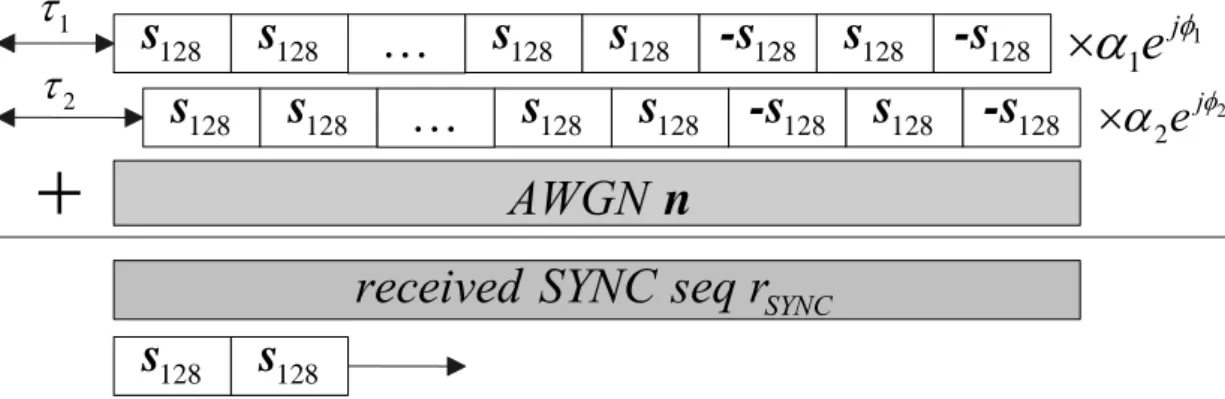
Figure 4.4 An example of received SYNC sequence in two-path channel

      A simple case is shown in the above figure. The synchronization sequence passes

through a two-path Rayleigh fading channel. Figure 4.4 also shows the relationship between

18  ]

the synchronization sequence and the received signal. To simplify the main topic, we ignore

the noise effect in the following deriving. We define the correlation filter window as

. Then we use the sliding window to calculate the cross-correlation of

128 128

[

sync =

s s s r_sync

and s_sync. We can expect that the peak value will occur when s_sync is perfectly matched to

the synchronization sequence in the r_sync. It means the peak value will occur at τ₁, τ₂,

1 128

τ + , τ2+128, , until the SFD appears.

Figure 4.5 is the channel impulse response, and figure 4.6a is the output sequence of

correlation detector. We can easily find that peak values occur repeatedly. We overlap the

channel impulse responses with processing gain 256 on the output sequence in figure 4.6b,

and find they are almost the same. When the SFD passes through the filter, the peak value will

occur with 180 degrees phase rotation. According to these peak values and the phase rotation,

we can easily find the position of the strongest path and the timings when channel estimation

sequence and data sequence come.

propagation delay

Figure 4.6a Output sequence of matched filter

Figure 4.6b Mapping the CIR on output of matched filter

However, if the strongest path is not the first path, then the symbol timing estimated may

be incorrect [5]. Due to this problem, the modified synchronization method is proposed to

increase the probability of tracking on the first path.

After we find the position ( ) of the strongest path, we need to check if there is

another path which is strong enough in the interval

max_pos

n

[nmax_pos−τmax ,nmax_pos] where τmax  is

the maximum delay of channel impulse response. Finally, we used the special assignment of

SFD to find the timing of synchronization sequence ends. We propose our synchronization

algorithm as table 4.1. Flow chart is shown in figure 4.7.

Frame Start Power accumulator

Find maximum value and position (Step 1)

Check pos-128 & pos+128 (Step 2)

First path check (Step 4)

Start frame delimiter (Step 5)

Y

Y

Y

Y

N

N

N

N

Start

Find first path position (Step 3)

Figure 4.7 Flow chart of synchronization algorithm

( ) max

Step 1:

find

max{

( [ ])}

find

max{

( [ ])}

Step 2:

if

( [

128])

||

( [

128])

else

[

]

0 and go s

max_pos max_pos max

first_pos max_pos max_pos

y

abs y i

n

abs y i

abs y n

y

abs y n

y

n

n

y n

α

α

=

=

−

>

+

>

=

=

Synchronization algorithm :

tep 1.

Step 3:

find

[ ]

,

from

to

and

Step 4:

if

( [

128]

) ||

( [

128]

)

.

else

[

]

0 and go step 3.

Step 5:

if (

( [

j max first_pos max first_pos

j pos

j pos max j pos max

first_pos j pos j pos fir

y

y j

y

j

n

n

n

j

abs y n

y

abs y n

y

n

n

y n

abs y n

γ

τ

γ

γ

=

≥

−

=

+

>

−

>

=

=

128])

)

and

else

=

+128 and go step 5.

first_pos first_pos Length

first_pos first_pos

y

CE timing = n

+ 256

Data timing = n

+CES

.

n

n

ρ

+

<

Table 4.1 Synchronization algorithm

4.3 Channel estimation

The issue of this section is to estimate channel impulse responses (CIRs) for later

applications. We use the special structure of CES in the PLCP preamble and the correlation

property of complementary sequences to develop our channel estimation scheme. Some

channel estimation and channel tracking methods which use Golay complementary code for

OFDM system can be found in [6] and [7]. We will introduce Golay complementary sequence

first, and then we will explain our algorithm for channel estimation.

4.3.1 Golay complementary code

A set of complementary series is defined as a pair of equally long, finite sequences of

two kinds of elements which have the property that the number of pairs of like elements with

any given separation in one series is equal to the number of pairs of unlike elements with the

same separation in the other series [8]. For example, the two series A=00010010 and

B=0011101 are complementary.

Binary complementary code can be defined as follow. Let us consider a pair of equally

long sequences{ [ ]}α n and{ [ ]}β n ,  for 0≤ ≤ − ,  where N is the length of two sequences. n N 1

These sequences are called complementary codes if their auto-correlations satisfy the

relationship shown in equation 4.3.

1 * * 0 [ ] { [ ] [(( )) ] [ ] [(( )) ]} 2 [ ] 2 , 0 (4.3) 0, 0 N N N m n m m n m m n N n N n n α α β β δ − = Γ − + − = = ⎧ = ⎨ _≠ ⎩

∑

where ( )⋅* denotes the complex conjugate operation, and δ[ ]n is the Kronecker delta

function. The auto-correlation of complementary sequences defined in IEEE 802.15.3c

standard is shown in figure 4.8.

peak value

interference free region

Figure 4.8 Auto-correlation of complementary codes with length 256

4.3.2 Channel estimation scheme

In IEEE 802.15.3c standard, the channel estimation sequence (CES) consists of one pair of complementary sequences (a₂₅₆ and  b256). Figure 4.9 shows the structure of CES, where

256, pos

a , a_{256, pre}, b_{256, pos} , and b_{256, pre} are the last and first half part of and ,

respectively.

256

256

a

a

a

b

b

b

Figure 4.9 Structure of IEEE 802.15.3c SCBT CE sequence

According to this special arrangement, we can use the auto-correlation property that we

introduced in the previous section to implement our channel estimation algorithm. Figure 4.10

shows a simple example for our channel estimation scheme. The received CES   is the

summation of CESs with different delay arguments, gains, and phases and AWGN . In this

section, we assume the synchronization block can provide perfect timing for channel

estimation. By using this special structure of CES, the received CES can be represented

as CE r n CE r 256 1 256 1 [(( 1 )) 1] , 1 256 [ ] (4.4) [(( 1 512 )) 1] , 513 768. l l L j l l l CE _L j l l l a n e n r n b n e n φ φ τ α τ α = = ⎧ _{− − + ≤ ≤} ⎪⎪ = ⎨ ⎪ _{− − − + ≤ ≤} ⎪⎩

∑

∑

e

α

×

e

α

×

e

α

×

+

Figure 4.10 An example of channel estimation scheme 24 

By using the correlation scheme (or matched filter), we can calculate the correlation between

and  [  

CE

r a₂₅₆ 0  ₂₅₆ ].  If we know the maximum channel delay which is smaller than CP

length in general, then output sequence of matched filter can be modified as   

256 b 256 256 256 1 1 768 256 256 513 1 1 [ ] ( [(( 1 )) 1] [(( 1 )) 1]) ( [(( 512 )) 1] [(( 512 )) 1]) 512 [ ] (4.5) l l l L j l l n l L j l l n l L j l _l l c m a n e a n m b n e b n m e m φ φ φ τ α τ α α δ τ = = = = = = − − + − − + + − − + − − + = −

∑ ∑

∑ ∑

∑

for 1≤ ≤m τ_max, where αl, φ , and _l τl are estimated channel gain, phase, and delay,

respectively.

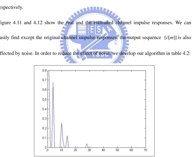
Figure 4.11 and 4.12 show the real and the estimated channel impulse responses. We can

easily find except the original channel impulse responses, the output sequence is also

affected by noise. In order to reduce the effect of noise, we develop our algorithm in table 4.2:

{ [ ]}c m

Figure 4.11 Original channel impulse responses

noise

γ

Figure 4.12 Estimated channel impulse responses with noise

[ ]

Step 1.

Calculate [ ] for 1

delay maximum.

Set

max{

( [ ])} & path number

Step 2.

for

1: delay maximum

if ( [ ]

)

[ ]

[ ] / 512

path number=path number+1

else

[ ]

0

end

c m

m

abs c m

= 0.

i

c i

c i

c i

c i

γ

γ

γ

≤ ≤

=

=

>

=

=

Channel estimation algorithm :

Table 4.2 Channel estimation method

Define the accepted threshold γ_th can help us to filter the noise effect and estimate the more

accurate channel impulse responses.

After estimating the channel impulse responses by the above method, we also need to

estimate the noise power for the following section. From above, we know the elements in

sequence { [ ]}c m their absolute values under the threshold γ_thare constructed of i.i.d AWGN

with zero mean and 0

2

N

variance. We derive the noise statistic as follow:

Assume and are both Gaussian random variables with zero mean and

variance. Ii n n_Qi N₀/ 2 512 1 ( ) ( j _{i Ii Qi} Ij Qj i n c n jn n jn = =

∑

∑

∑

512 512 1 1 [ Ij] _{i Ii i} [ _Ii] 0, (4.7) i i E n E c n c E n = = ⎡ ⎤ = _{⎢ ⎥}= = ⎣

∑

∑

∑

∑ ∑

Furthermore, the elements in complementary sequences   and  are either +1 or

-1, so the complexity of this channel estimation scheme can be much reduced by replacing

multiplication by inverter and summation. Because of this characteristic, we can reduce the

complexity in circuit design and make it more suitable for high speed signal processing.

Finally, we modify our scheme and show it in table 4.3.  

256

a b₂₅₆

max 2 [ ] max 2 2 ₂

Step 1:

Calculate [ ] for 1

.

Set

max{

( [ ])},

0, and

0

Step 2:

for

1:

if ( [ ]

)

[ ]

[ ] / 512 and

1

else

=

+ c[ ] /512 and [ ]

0

e

c m

m

abs c m

path

i

c i

c i

c i

path

path

i

c i

τ

γ

γ

σ

τ

γ

σ

σ

≤ ≤

=

=

=

>

=

=

=

Channel estimation algorithm :

=

+

nd

Step 3:

[ ] and

/(

)

e

c l

path

α

=

σ

=

σ

τ

−

Table 4.3 Modified channel estimation method

4.4 Equalization

After above two sections, we get the time of data sequence arriving, the estimated CIR,

and estimated noise power. Now we need to equalize the channel effect on received data

sequence caused by multipath fading channel. There are several equalization methods such as

decision feedback equalizer which is proposed in [9]. However, according to the specification

that published by IEEE 802.15.3c working group, we use the frequency domain equalizer

(FED) to compensate the channel effect.

The SCBT with FDE is very similar to OFDM since both of them perform channel

equalization in frequency domain. Their difference is the position of IFFT operation. In SCBT

with FDE, IFFT is placed in the receiver, between the equalization and data decision. The

block diagram of FDE is shown in figure 4.13.    

In figure 4.13, we show the block diagram of SCBT with FDE. Take the k-th block of the

received signal as an example. After removing the CP, this N-length block can be written in

vector form

T

[ [ , 0] [ ,1] [ , 1]] (4.9)

k y k y k y k N−

y

where is the  n-th symbol in the k-th data block. For simplicity, we drop the block

index k and the original vector becomes

[ , ] y k n T [ [0] [1]y y y N[ −1]] . (4.10) y  

⊗

⊗

⊗

y

x

Figure 4.13 The block diagram of FDE

Through  N‐length FFT, the time domain vector is transformed into frequency domain and

represented as y T [ [0] [1]Y Y Y N[ −1]] (4.11) Y   29 

where Y n[ ]  is the signal at n-th subcarrier which can be expressed as 1 0 2 [ ] [ ]exp( ). (4.12) N l j nl Y n y l N π − = =

∑

Suppose the originally sent data block is

T

[ [0] [1]x x x N[ −1]] . (4.13)

x  

And its corresponding frequency domain vector is

T

[ [0]X X[1] X N[ −1]] . (4.14)

X  

Hence, the original and received frequency domain signals at the n-th subcarrier have the

following relationship

[ ] [ ] [ ] [ ] (4.15)

Y n =H n X n +N n  

where and   are channel frequency response (CFR) and noise at the  n‐th

subcarrier respectively.

[ ]

H n N n[ ]

The FDE can be realized as an N-branch linear feed-forward equalizer with W[n] as

complex coefficient at the n-th subcarrier. Transforming the equalized frequency domain

signal back into time domain by IFFT operation, we have

1 0 1 2 [ ] [ ] [ ]exp( ). (4.16) N l j nl x n W l Y l N N π − = − =

∑

The equalized time domain data block

T

[ [0] [1]x x x n[ ]] (4.17)

x  

can be sent to the hard decision device for data decision or further processing.

The linear FDE can take form of either zero forcing (ZF) or minimum mean-square error

(MMSE). If optimized based on ZF criterion, the FDE coefficient W[n] is 1 [ ] . (4.18) [ ] zf W n H n =  

If optimized based on MMSE criterion, the FDE coefficient W[n] becomes

* 2 [ ] [ ] (4.19) | [ ] | 1/ mmse H n W n H n η = +   where  _{η   denotes SNR.}

In severe frequency selective fading where the spectral null (deep fading) occurs, the

inversion of H[n] in ZF-FDE leads to infinity and results in noise enhancement at those

frequencies of spectral null. MMSE-FDE is more appealing since it can make compromise

between the residual inter-symbol interference (ISI) (in the form of gain and phase

mismatches) and noise enhancement. Therefore, it can minimize the combined effect of ISI

and noise. This is particularly attractive for equalizing the channels of severe frequency

selective fading. According to past studies, MMSE-FDE has significantly better performance

than ZF-FDE for SCBT systems. However, MMSE-FDE needs to know SNR. The accuracy

of SNR estimation affects the performance of MMSE-FDE [10]. The simulation result of

MMSE-FDE and ZF-FDE is shown in figure 4.14.

Figure 4.14 Performances of MMSE-FDE and ZF-FDE in 6-path channel

4.5 Data detection

In this section, we introduce some methods to improve the performance after FDE.

According to the definition of the SCBT system, the relationship between received and

transmitted signal can be written in matrix form as follow:

1 1 2 1 1 2 2 1 2 2 2 1 (4.20) L L L L N L N N y h h h x n y h h x n h y h y h h h x n ⎡ ⎤ ⎡ ⎤⎡ ⎤ ⎡ ⎤ ⎢ ⎥ ⎢ ⎥⎢ ⎥ ⎢ ⎥ ⎢ ⎥ ⎢ ⎥⎢ ⎥ ⎢ ⎥ ⎢ ⎥ ⎢ ⎥⎢ ⎥ ⎢ ⎥ = + ⎢ ⎥ ⎢ ⎥⎢ ⎥ ⎢ ⎥ ⎢ ⎥ ⎢ ⎥⎢ ⎥ ⎢ ⎥ ⎢ ⎥ ⎢ ⎥⎢ ⎥ ⎢ ⎥ ⎢ ⎥ ⎢ ⎥⎢ ⎥ ⎢ ⎥ ⎢ ⎥ ⎢ ⎥ _{⎣ ⎦}⎢ ⎥ ⎢ ⎥ ⎣ ⎦ ⎣ ⎦ ⎣ ⎦  

where y , _n x , and _n are received signal, transmitted signal, and i.id AWGN noise

respectively.

n

n

From equation 4.20, the posteriori distribution can be expressed as / 2 2 / 2 2 1 1 ( | ) exp( ( ) ( )). (4.2 (2 ) ( ) 2 H N N p H H π σ σ = − − − y x y x y x 1)

In general, the best data detection performance is provided by maximum likelihood (ML)

detector whose detection rule can be expressed as

( ) ( ) max ( | ). (4.22) i i ML = p x x y x  

To maximize the conditional probability in the above equation is equivalent to minimize the

following equation: ( ) ( ) ( ) min(_i i ) (H i ). (4.23) ML = −H −H x x y x y x

However, when the size of x becomes large, the ML detector may be too complex to be

implemented in practical.

In this section, in order to focus on the data detection methods, we assume that the

channel state information (CSI) is perfectly known by the receiver.

4.5.1 Gibbs sampler (GS)

Gibbs sampler is an application of Markov Chain Monte Carlo method which is

proposed in statistics first. It is used for approaching the complex probability distribution by

drawing the samples from a simple probability distribution. In other words, the Gibbs sampler

is a technique for generating random variables from a marginal distribution indirectly, without

having to calculate the density [11].We will introduce the Markov Chain Monte Carlo method

before we look into the Gibbs sampler in detail at later of this section.

4.5.1.1 Markov Chain Monte Carlo method (MCMC)

Before we mention the details of Gibbs sampler, we take a look on how a probability

distribution can be approximated by generating random samples. Bayesian approach is a

common method used in data detection, but usually needs high dimension of integration

which is too complex to be implemented on hardware. Therefore, we introduce the Markov

Chain Monte Carlo method to reduce the complexity of computation.

First, we introduce the Monte Carlo integration which is developed for high dimensional

integration, the equation of Monte Carlo integration can be expressed as

( ) ( ) ( ) ( ) [ ( )] (4.24) b b p x ah x dx= a f x p x dx E= f x

∫

∫

where p(x) is a probability density function defined in [a,b].

As the equation mentioned above, if we draw samples _x( )i

  from probability density

function ,  and the number of samples is large enough. Then the integration of can

be expressed as ( ) p x h x( ) ( ) ( ) 1 1 ( ) ( ) [ ( )] ( ). (4.25) N b _i p x a i f x p x dx E f x f x N = = ≅

∑

∫

Moreover, we derive the conditional probability as follow:

( ) ( ) 1 1 ( | ) ( ) [ ( | )] ( | ). (4.26) N b _i p x a i f y x p x dx E f y x f y x N = = ≅

∑

∫

Equation 4.24 is called Monte Carlo integration

35 

)

t

j

After mentioning about Monte Carlo integration, then we introduce the Markov Chain.

We use the following equation to describe a Markov Chain process

  where    presents the

sample of a variable x at time t and Pr is the transition probability. In other words, each

sample of variable in Markov Chain is correlated only with the former sample .

1 1 0 0 1 1 1 1 Pr(Xt+ =st+ |X =s X, =s, ,Xt =st)=Pr(Xt+ =st+ |Xt =s 1 t X₊ t X t X

Now, we define the transition probability as p i j( , )=Pr(X_t+₁ =s X_j| _t =s ) , 

andπ_j( )t =Pr(X_t =s_j)presents the state of the Markov Chain is s_j  at time t. One important

property of Markov Chain is when Markov Chain becomes stable

( πk(t n+ )=πk( )t =πk forn 0

,

P_{k j k} P_{j k}

≥

, j

), then it must satisfy the detailed balance

function π = π . The proof of detailed balance function is derived as

, , , P P P . (4 j k j k j k j j j k j k k k π =

∑

∑

∑

4.5.1.2 Gibbs sampler

The Gibbs sampler was proposed by Geman in 1984 for image processing. It is a special

case from Metropolis-Hastings algorithm with accepted ratio α   always equals to 1. In other words, the samples generated by the transition probability will always be accepted. If the

number of samples that we generated is large enough, then we can approach the target

distribution by Monte Carlo method. The algorithm can be developed and demonstrated in

(0) (0) (0) (0) T 1 2 N 0 (n) (n-1) (n-1) (n-1) 1 1 2 3 N (n ) 2

Given the initial values [ ] , the algorithm iterates the following loop from n 1 to n n +Ns.

Draw sample from ( | , , , ). Draw sample from (

x x x x p x x x x x p = = = • • … x y (n ) (n-1) (n-1) 2 1 3 N (n ) (n ) (n ) (n ) N N 1 2 N-1 | , , , , ).

Draw sample from ( | , , , , ).

Samples from the last Ns iterations are used to calculate the Bayesian estimates of the u x x x x x p x x x x • … … y y 0 0 0 n +Ns (n) n=n +1

nknown quantities.The initial period of length n is known as the "burn-in" period.

1 ( ) ( | ) ( ) f p d x f N ⇒

∫

∑

Table 4.4 General Gibbs Sampler algorithm

According to the equation 4.21 at the beginning of this section, we know that

2 1 ( | ) exp( ( ) ( )). (4.28) 2 H p H H σ ∝ − − − y x y x y x . 

To start the Gibbs sampler process, we need to calculate the probability density function (PDF) 

1 1 1

( _n| , , , _n , _n , , _N)

p x y x x ₋ x ₊ x . As the derivation in [12], we derive target PDF as follow:

1 1 1 1 1 1 1, 1, 1 ( | ) ( ) ( | , , , , , , ) ( , , , , , , ) ( | ) ( ) ( , , , ) n n n N n n N n n n N p p p x x x x x p x x x x p p x p x x x x − + − + − + = = y x x y y y x 1, 1, 1 1, 1, 1 ( | , _{n n} , , _N) ( , _{n n} , , _N) p y x x ₋ x ₊ x p x x ₋ x ₊ x 1 1 1 1 ( | ) ( ) (4.29) ( | , , , , , , ) ( ) n M n n i n N n i i p p x p x x ₋ x m x₊ x p x m = = = =

∑

where mi  is the possible symbol of x , and M is the total number of possible symbols of x. n

If the probability for all i are equally likely which is suitable for general cases in

communication engineering. Then we can continue to derive above equation as ( n i

p x = )m

1 1 1 ( | ) ( | , , , , , , ) . (4.30) ( | ) n n n n N x p p x x x x x p − + =

∑

For example, in BPSK transmission,

1 1 1 1 ( | ) ( 1| , , , , , , ) . (4.31) ( | ) n n x n n n N x p p x x x x x p = − + = =

∑

Then the ratio 1/D which is defined as _n 1 1 1

1 1 1 ( 1| , , , , , , ) ( 1| , , , , , , n n n n n n p x x x x x p x x x x x − + − + ) N N = = − y y can be derived as 1 1 1 1 1 1 2 2 2 1 1 ( 1| , , , , , , ) 1/ ( 1| , , , , , , ) 1 exp( ( )). (4.32) 2 n n n n n N n n n n N x x p x x x x x D p x x x x x H H σ − + − + = =− = = = − = − − − − y y y x y x  

After we get the above probabilities, we draw a sample from random variable U which is

uniformly distributed in an interval [0,1]. And we decide the value of sample

n u n x by following rule: ( ) 1 1, if 1 = . ( 1, Otherwise n i n n u D x ⎧ _< ⎪ ₊ ⎨ ⎪ − ⎩ 4.33)  

According to the above derivation, we conclude our Gibbs sampler detector algorithm for

SCBT system in BPSK transmission in table 4.5.

To compute the number of multiplications in Gibbs sampler detector, we found to

calculate ( ) 2 1 i n x H ₌ −

y x need 2P multiplications, where P is the number of paths. In general,

  multiplications per iteration and

2P M× ×N 2P M×   multiplications per symbol are

needed, where M is the number of transmitted symbols, N is the length of data symbols. If the

Gibbs sampler iterates Ns times, there are 2P M N Ns× × × multiplications in this process.

More detail in calculation for number of multiplications is shown in appendix A.

( ) ( ) (0) (0) (0) 1 0 2 1 Step 1.

Start with an initial values [ , Calculate Step 2. for 1 ~ ( ) for 1 ~ Calculate i i n n P p p n x x Hx x h i n Ns n N d H H = = = = = + = = − − −

∑

Gibbs sampler algorithm (BPSK tr

x y x y x (0) (0) 1 2 , ] . T N x x x ansmission) 2 2 ( 1) 1 2 ( 1) 1 ( ) ( ) ( ) ( 1) 1 1 ( ) ( 1 ( [(( 2)) 1] 1] ( [ ] 1) ) ( [(( 2)) 1] 1] ( [ ] 1) ) Calculate ( 1| , , , , ( 1| , s s P n p N p N p p P n p N p N p p i i i n n i i n y n h x n y n h x n p x x x x p x x − = − = − + = + − + − + + − − + − + − + + + = = −

∑

∑

τ

τ

τ

τ

Draw a random value ~ (0, 1 1, if 1 = 1, Otherwise end end Step 3.

Take the last Ns samples ~ on by the follo

i n n i i n n n n i n n n d D x x u U u D x

σ

, and make decisi

i N x − − wing rule: 1 , ( 1) ( 1 . 1 , n n i i i if num x num x x othrwise ⎧ = > = − = ⎨ − ⎩ ) 38   

Table 4.5 Gibbs Sampler algorithm in SCBT data detection

There are some problems need to be discussed when using Gibbs sampler in our system.

One is the number of burn-in period and total samples. It would become a tradeoff between

complexity and performance. The fewer samples we take the lower complexity we have, but it

leads the poor performance and vice versa. In this case, we can use experience to find the best

performance on the constraint of computation complexity or efficiency to solve this problem.

The other problem is the selection of initial values. The past studies had shown that the

Gibbs sampler performs well in low SNR region, it may suffer from a noise floor, or even its

performance may degrade as SNR increase. At high SNR region, some of the transition

probabilities in the underlying Markov Chain may become very small. It leads the Markov

Chain may be divided into several disjoint chains. As the result, a Gibbs sampler which starts

from a random initial set will remain within the set surrounding the initial set. Then this chain

may converge at local minimum and become stable [13]. To face this situation, we can use

some simple method to get a set of initial values around the global optimum. Developed in

our system, the result by making hard decision after FDE may be good enough to solve this

problem. Figure 4.15 shows the complete block diagram of the proposed Gibbs sampler

detector.

Figure 4.15 The block diagram of our Gibbs Sampler detector 39