國 立 交 通 大 學
電信工程學系碩士班
碩士論文
IEEE 802.11n
多重輸出輸入最佳化接收器設計
Optimum MIMO Receiver for IEEE 802.11n System
研 究 生:吳俊穎
指導教授:吳 文 榕 博士
IEEE 802.11n 多重輸出輸入最佳化接收器設計
Optimum MIMO Receiver Design for IEEE 802.11n System
研 究 生:吳俊穎 Student:Jiun-Ying Wu
指導教授:吳文榕 博士 Advisor:Dr. Wen-Rong Wu
國 立 交 通 大 學
電信工程學系碩士班
碩 士 論 文
A Thesis
Submitted to Department of Communication Engineering
College of Electrical and Computer Engineering
National Chiao-Tung University
in Partial Fulfillment of the Requirements
for the Degree of
Master of Science
In
Communication Engineering
July 2007
Hsinchu, Taiwan, Republic of China
IEEE 802.11n 多重輸出輸入最佳化接收器設計
研究生:吳俊穎 指導教授:吳文榕 教授
國立交通大學電信工程學系碩士班
摘要
IEEE 802.11n 使用了正交分頻多工 (OFDM) 與多重輸入輸出
(MIMO) 作為其基頻之傳輸模式。與傳統的無限網路系統相比,
802.11n 可以提供更為高速的傳輸速度。然而,多重輸入輸出接收器
的設計是一個非常困難的工作。最大相似度 (ML) 接收器擁有最好的
效能,但是卻要付出極高的複雜度去實現。球型接收器 (SD) 可以有
效的簡化運算複雜度,然而其運算量非常不固定,不利於硬體上之實
現。在本論文中,我們將提出一個新的演算法來解決這個問題。我們
所提出的演算法,在效能上能接近最佳的ML 接收器,並且可以大幅
降低複雜度;與SD 相比,我們提出的演算法擁有固定的運算量。另外
一個優點是,我們提出的演算法,可以容易的在複雜度與效能中做出
取捨。除此之外,我們可以延伸此演算法來計算軟性位元,以提供軟
性解碼器之使用。模擬的結果顯示出,在與傳統的方法(最小均方差
等化器(MMSE))相比,我們所提出的演算法在效能上能有超過10 dB
的提升。
Optimum MIMO Receiver Design for IEEE 802.11n System
Student:
Jiun-Ying
Wu
Advisor:
Dr.
Wen-Rong
Wu
Department of Communication Engineering
National Chiao-Tung University
Abstract
IEEE 802.11n uses the multiple input multiple output (MIMO) with
orthogonal frequency division multiplexing (OFDM) as its transmission
scheme. Compare with conventional wireless network system, IEEE
802.11n can provide a very high throughput. However, the receiver
design for MIMO systems remains a very challenging task. As we known,
the maximum-likelihood detector (MLD) is the optimum receiver, but the
cost of implementation is very high due to its high complexity. In this
thesis, we propose a new algorithm to overcome the problem. The
proposed algorithm can achieve the performance of MLD, and reduce the
complexity significantly. Meanwhile, the throughput of the proposed
algorithm is constant, and it can be easy to change complexity by
modifying the parameter in our algorithm. Simulation with 802.11n
system shows that our proposed algorithm has significant gain compared
with conventional method.
誌謝
本篇論文得以順利完成,首先要特別感謝我的指導教授 吳文榕
博士,在課業學習與論文研究上不厭其煩的引導我正確的方向。
另外,我要感謝許兆元學長、謝弘道學長、李俊芳學長與楊華龍
學長等在研究上不吝指導,且同時感謝寬頻傳輸與訊號處理實驗室所
有同學與學弟妹們的幫忙。
Contents
1 Introduction 1
2 IEEE 802.11n Transmitter Overview 4
2.1 Introduction . . . 4 2.2 Packet Format . . . 4 2.3 Cyclic Shift . . . 5 2.4 High-Throughput Preamble . . . 6 2.4.1 HT SINGAL Field . . . 7 2.4.2 HT-STF training symbol . . . 9 2.4.3 HT-LTF training symbol . . . 9 2.5 Data Field . . . 9 2.5.1 Scrambler . . . 9 2.5.2 FEC . . . 10 2.5.3 Stream Parser . . . 12 2.5.4 Frequency Interleaver . . . 12 2.5.5 QAM Mapping . . . 13 2.5.6 OFDM modulation . . . 15 2.6 Channel Model . . . 15
3 IEEE 802.11n Receiver Design 17 3.1 Packet Detection . . . 17
3.2 Frequency Synchronization . . . 19
3.3 Symbol Timing Offset . . . 21
3.5 Phase Tracking . . . 24
3.6 Sampling Frequency Offset . . . 25
4 MIMO Detector 27 4.1 Problem Definition . . . 27
4.2 Maximum Likelihood Detector . . . 28
4.3 Sphere Decoding . . . 28
4.4 Proposed Method . . . 31
4.5 Complexity Analysis . . . 35
4.6 Simulations . . . 37
5 MIMO Soft Bit Demapping 45 5.1 Bit-interleaved Coded Modulation . . . 45
5.2 Log Likelihood Ratio . . . 45
5.3 List Sphere Decoding . . . 47
5.4 Soft Output of Proposed Algorithm . . . 48
5.5 Simulations . . . 50
6 Simulations With IEEE 802.11n System 59 7 Conclusions 66 7.1 Conclusion . . . 66
List of Figures
1 802.11n Block Diagram . . . 4
2 802.11n Packet Format . . . 5
3 HT Singal Field . . . 8
4 Constellation for Legacy Signal Field and the HT signal Field 8 5 Data Scrambler . . . 10
6 Convolution Encoder . . . 10
7 Punture Process . . . 11
8 QAM Modulation . . . 14
9 Singal flow structure of the delay and correlation algorithm . . 17
10 Process of Packet Detection . . . 18
11 Preamble for CFO Estimation . . . 20
12 Preamble for Symbol Timing . . . 22
13 Histogram of Number of Candidates . . . 31
14 Projection in each group . . . 32
15 BER comparison for 2 × 2 16-QAM(I) . . . 39
16 BER comparison for 2 × 2 16-QAM(II) . . . 39
17 BER comparison for 3 × 3 16-QAM(I) . . . 40
18 BER comparison for 3 × 3 16-QAM(II) . . . 40
19 BER comparison for 4 × 4 16-QAM(I) . . . 41
20 BER comparison for 4 × 4 16-QAM(II) . . . 41
21 BER comparison for 2 × 2 64-QAM(I) . . . 42
22 BER comparison for 2 × 2 64-QAM(II) . . . 42
24 BER comparison for 3 × 3 64-QAM(II) . . . 43 25 BER comparison for 4 × 4 64-QAM(I) . . . 44 26 BER comparison for 4 × 4 64-QAM(II) . . . 44 27 BER comparison of soft demapping for 2 × 2 16-QAM system(I) 52 28 BER comparison of soft demapping for 2×2 16-QAM system(II) 52 29 BER comparison of soft demapping for 3 × 3 16-QAM system(I) 53 30 BER comparison of soft demapping for 3×3 16-QAM system(II) 53 31 BER comparison of soft demapping for 4 × 4 16-QAM system(I) 54 32 BER comparison of soft demapping for 4×4 16-QAM system(II) 54 33 BER comparison of soft demapping for 2 × 2 64-QAM system(I) 55 34 BER comparison of soft demapping for 2×2 64-QAM system(II) 55 35 BER comparison of soft demapping for 3 × 3 64-QAM system(I) 56 36 BER comparison of soft demapping for 3×3 64-QAM system(II) 56 37 BER comparison of soft demapping for 4 × 4 64-QAM system(I) 57 38 BER comparison of soft demapping for 4×4 64-QAM system(II) 57 39 BER comparison of hard decision and soft demapping for 3×3
64-QAM system . . . 58 40 BER comparison of hard decision and soft demapping for 4×4
64-QAM system . . . 58 41 PER comparisons of Proposed Algorithm, LSD and MMSE
(20MHz, 4 × 4, 64QAM, 5/6 code rate, Channel B) . . . 61 42 PER comparisons of Proposed Algorithm, LSD and MMSE
43 PER comparisons of Proposed Algorithm, LSD and MMSE (20MHz, 4 × 4, 64QAM, 5/6 code rate, Rayleigth uncorrelated Channel) . . . 63 44 PER comparisons of Proposed Algorithm, LSD and MMSE
(20MHz, 4 × 4, 64QAM, 1/2 code rate, Rayleigth uncorrelated Channel) . . . 64 45 PER comparisons of Proposed Algorithm, LSD and MMSE
(20MHz, 2 × 2, 16QAM, 1/2 code rate, Rayleigth uncorrelated Channel) . . . 65
List of Tables
1 Cyclic shift for non- HT portion of the packet . . . 6
2 Cyclic shift for HT portion of the packet . . . 6
3 Normalization Factor . . . 13
4 Pliot Value for 20MHz . . . 15
5 Pliot Value for 40MHz . . . 16
6 Number of Multiplications required in proposed and ML algo-rithm . . . 37
7 Number of Multiplications required in proposed and SD algo-rithm . . . 37
1
Introduction
In recent years, wireless data communication has been grown extensively. As a result, existing wireless communication systems can not satisfy the fast-growing demand. It is know that increasing the bandwidth can effec-tively increase the data transmission rate. However, the resource for wireless communication is limited. Thus, how to improve the spectrum efficiency of wireless communication systems becomes an important issue.
One effectively way to improve capacity is to use the multiple transmit and receive antennas, resulting in multi-input multi-output (MIMO) systems. Conventionally, the communication system is implemented as a single-input single-output (SISO) system. In 1998, Telartar and Foschini have shown that the MIMO channel capacity can grow approximately linearly with the num-ber of antennas used [1], [2]. MIMO techniques can basically group into two categories. The first one aims to improve the power efficiency and transmis-sion reliability by maximizing spatial diversity. One popular example of such a system is the space-time block codes (STBC) [3]. The second category uses a layered approach to increase capacity. One popular example is the vertical-Bell Laboratories layered space-time (V-BLAST) architecture [4], [5]. In this case, independent data streams are transmitted over different antennas to increase the data rate.
Another way to enhance the spectrum efficiency is to use the orthog-onal frequency division multiplexing (OFDM) technique. This technique, proposed by Salzberg in 1967 [6], evolves to becomes a digital multi-carrier modulation scheme. The main idea of ODEM is to spilt a high rate stream
into a number of low rate streams, and transmit them simultaneously over different sub-carriers. Each sub-carrier is modulated with a conventional modulation scheme, maintaining its data rate similar to conventional single-carrier modulation scheme in the same bandwidth. The primary advantage of OFDM is its ability to convert the multi-path frequency-selective fading channel into a number of flat sub-channels. The receiver can easily adapt to channel conditions with simple equalization. In implementation, OFDM symbols can be generated by the efficient Fast Fourier transform (FFT) algo-rithm. Nowadays, OFDM has developed into popular schemes for wideband digital communication systems, such as terrestrial digital video broadcasting (DVB-T), the IEEE 802.11a/g wireless local area network (WLAN) and the IEEE 802.16e Worldwide Interoperability for Microwave Access (WiMAX) Wireless MANs. Combining with the MIMO structure, OFDM can further enhance the spectrum efficiency. The MIMO-OFDM scheme has been con-sidered as the main solution for enhancing the data rates in next-generation wireless communication systems, such as IEEE 802.11n High Throughput WLAN and the Fourth-Generation Cellular Communications System (4G).
However, the receiver design for MIMO systems between the cost-performance tradeoff remains a very challenging task. The maximum-likelihood detector (MLD) is the optimum receiver, but the cost of implementation is very high due to its high complexity. Another popular approach is called sphere decod-ing (SD) [7]; it can achieve the performance of MLD and significantly reduce the computational complexity. But the disadvantage is that the through-put of SD is not constant, it is difficult to have an efficient hardware im-plementation. In this thesis, we propose a new algorithm to overcome the
problem. The proposed algorithm can reach the performance of MLD, and reduce the complexity significantly. Meanwhile, the throughput of the pro-posed algorithm is constant. We also extend this algorithm to accommodate the MIMO soft-bit demapping problem. This will be very useful in modern bit-interleaved coded modulation systems (BICM).
The rest of this thesis is organized as follows. In Chapter 2, we review the specification of 802.11n Draft 2.0, and the transceiver structure of 802.11n. In Chapter 3, we present the design of the receiver structure and describe synchronization method. In Chapter 4, we discuss the MIMO detection al-gorithm including MLD, SD and the proposed alal-gorithm. Also, we will show the simulation results, conduct performance comparison, and analyze com-putational complexity in this chapter. In Chapter 5, we extend the proposed algorithm to reduce the computational complexity in the MIMO soft-bit demapping problem. Finally, we give some conclusions and outline future works in Chapter 6.
2
IEEE 802.11n Transmitter Overview
2.1
Introduction
IEEE802.11n is the next generation wireless local area networks (WLAN) standard. The transmission technique is similar to the previous IEEE802.11a standard, except for that the MIMO (multiple-input multiple-output) tech-nology is introduced. The MIMO techtech-nology uses multiple transmitter and receiver antennas to increase data throughput (with spatial multiplexing), or increase range (with space-time coding).
The publication of the standard is currently expected in September 2008. In this thesis, we will target on the latest specification ”IEEE 802.11n Draft 2.00”.
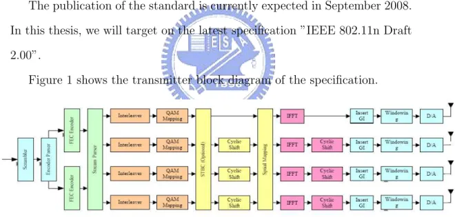
Figure 1 shows the transmitter block diagram of the specification.
Figure 1: 802.11n Block Diagram
2.2
Packet Format
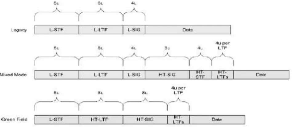
There are three kinds of packet format shown in fig.2. The elements of packets are:
Figure 2: 802.11n Packet Format
L-LTF: Legacy Long Training Field L-SIG: Legacy Singal Field
HT-SIG: High Throughput Singal Field HT-STF: High Short Training Field HT-LTF1: First High Long Training Field HT-LTF’s: Additional High Long Training Field Data: The Data Field
2.3
Cyclic Shift
Cyclic shifts are used to prevent unintentional beamforming when the same signal or scaled multiples of one signal are transmitted through different spatial streams or transmit chains. A cyclic shift of duration TCS on a signal
s(t) on interval 0 ≤ t ≤ T is defined as follows,
scs(t) =
½
s(t − TCS) TCS < t ≤ T
s(t − TCS+ T ) 0 ≤ t ≤ TCS (1)
Table 1: Cyclic shift for non- HT portion of the packet
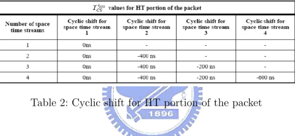
Table 2: Cyclic shift for HT portion of the packet
Table 1 specifies the values for the cyclic shifts that are applied in the non-HT short training field (in an non-HT mixed format packet), the non-non-HT long training field, and non-HT SIGNAL field. It also applies to the HT SIGNAL field in an HT mixed format packet. The values of the cyclic shifts to be used during the HT portion of the HT mixed format preamble and the data portion of the frame are specified in Table 2.
2.4
High-Throughput Preamble
The high throughput (HT) preambles are defined in HT mixed and in green-field formats to carry the required information to operate in a system with multiple transmit and multiple receiver antennas.
preamble compatible with the legacy mode. The legacy Short Training Field (L-STF), the legacy Long Training Field (L-LTF) and the legacy signal field are transmitted, so they can be decoded by legacy 802.11a/g devices. The rest of the packet has a new format. In this mode, the receiver shall be able to decode both the Mixed Mode packets and legacy packets.
In the greenfield format, all of the non-HT fields are omitted. The specific HT fields used are:
- HT SIGNAL Field(HT-SIG): provides all the information required to in-terpret the HT packet format,
- One HT Short Training Field (HT-STF) for automatic gain control (AGC) convergence, timing acquisition, and coarse frequency acquisition,
- One or several HT Long Training Fields (HT-LTF): provided as a way for the receiver to estimate the channel between each spatial mapper input and receive chain. The first HT-LTFs (Data HTLTFs) are necessary for demod-ulation of the HT-Data portion of the PPDU, and are followed, for sounding packets only, by optional HT-LTFs (Extension HT-LTFs) to sound extra spatial dimensions of the MIMO channel.
2.4.1 HT SINGAL Field
The high-throughput signal field is used to carry information required to interpret the HT packet formats. The fields of the HT SIGNAL field are described in table
The HT-SIG is composed of two parts, HT-SIG1 and HT-SIG2, each containing 24 bits, as shown in Figure 3 (Format of HT-SIG1 and HT-SIG2). All the fields in the HT-SIG are transmitted LSB first, and HT-SIG1 is
Figure 3: HT Singal Field
transmitted before HT-SIG2.
The HT-SIG parts are encoded, interleaverd, BPSK mapped, and have pliots inserted following the steps described in IEEE 802.11a standard. The result of BPSK modulation constellation is rotated by 90 degree relative to the traditional constellation shown in Figure 4
2.4.2 HT-STF training symbol
The purpose of the HT STF training field is to improve AGC training in a multi transmit and multi-receive system. The duration of the HT-STF is 4µsec. The frequency sequence used to construct the HT-STF in 20MHz transmission is identical to the legacy STF; in 40MHz transmission the HT-STF is constructed from the 20MHz version by frequency shifting and dupli-cating, and rotating the upper sub-carriers by 90X.
2.4.3 HT-LTF training symbol
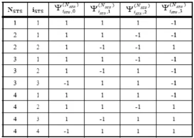
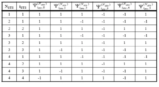
The HT long training field provides means for the receiver to estimate the channel between each spatial stream. In order to estimate all the response for each pass of the MIMO channel, the spatial-time mapping matrix is used. The mapping matrix PHT LT F
Hk= 1 −1 1 1 1 1 −1 1 1 1 1 −1 −1 1 1 1 (2)
2.5
Data Field
2.5.1 ScramblerThe DATA field shall be scrambled with a length-127 frame-synchronous scrambler. The octets of the PSDU are placed in the transmit serial bit stream, bit 0 first and bit 7 last. The frame synchronous scrambler uses the generator polynomial S(x) as follows, and is illustrated in Figure ??.
The 127-bit sequence generated repeatedly by the scrambler shall be (left-most used first), 00001110 11110010 11001001 00000010 00100110 00101110 10110110 00001100 11010100 11100111 10110100 00101010 11111010 01010001
Figure 5: Data Scrambler
10111000 1111111, when the all ones initial state is used. The same scram-bler is used to scramble transmit data and to descramble receive data. When transmitting, the initial state of the scrambler will be set to a pseudo random non-zero state. The seven LSBs of the SERVICE field will be set to all zeros prior to scrambling to enable estimation of the initial state of the scrambler in the receiver.
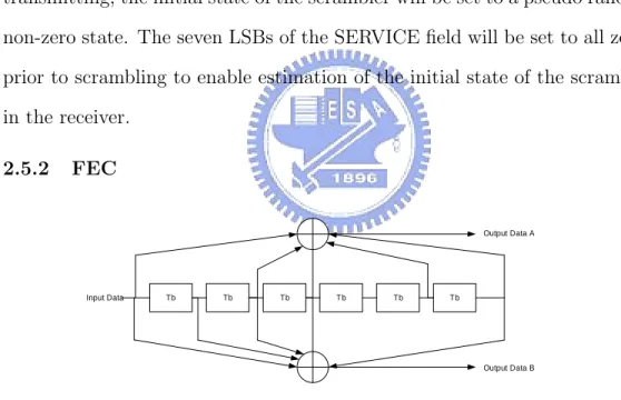
2.5.2 FEC
Input Data Tb Tb Tb Tb Tb Tb
Output Data A
Output Data B
Figure 6: Convolution Encoder
The mandatory coder is the convolutional code (CC) encoder and the optional one is a low-density parity-check (LDPC) encoder. We only focus our research in CC encoder. The CC encoder is defined by the Figure 6. A single CC encoder is used when Nss = 1 or Nss = 2, two CC encoders are
Coded Sequence Input Sequence I0 I1 I2 I3 I4 A0 A1 A2 A3 A4 B0 B1 B2 B3 B4 I0 I1 I2 I3 I4 A0 A1 A2 A3 A4 B0 B1 B2 B3 B4 Punctured Sequence : R=5/6 R=2/3 I0 I1 I2 I3 I4 I0 I1 I2 I3 I4 II5 1338 1718 1338 1718 A0B0A1B2A3B4 1338 1718 1338 1718 A0 A1 A2 A3 A4 B0 B1 B2 B3 B4 A0 A1 2 A3 4 B0 B1 B2 B3 B4 A5 B5 B A0B0A1A2B2A3A4B4A5 R =3/4 I0 I1 I2 I3 I4 I0 I1 I2 I3 I4 II5 1338 1718 1338 1718 A0 A1 A2 A3 A4 B0 B1 B2 B3 B4 A0 A1 2 A3 4 B0 B1 B2 B3 B4 A5 B5 B A0B0A1B2A3B3A4B5A6B6A7B8 Coded Sequence Input Sequence Punctured Sequence : I6 I7 I I II8 A6 A7 B6 B7 A B B A8 B8 B
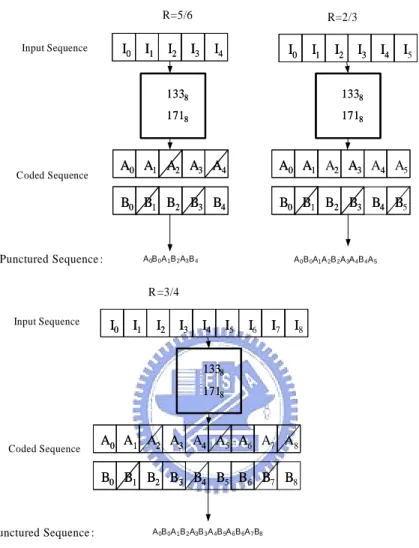
Figure 7: Punture Process
If two encoders are used, the data scrambled bits are divided between the encoders by sending alternating bits to different encoders.
The CC encoder output only provides the encoding output with 1 2 code
rate. In order to support a variable code rate, we can use puncture operation after encoding. The procedure of puncturing is shown in Figure 7. There are three kinds of code rates (2
2.5.3 Stream Parser
After coding and puncturing, the data bit streams at the output of the CC en-coders are parsed to multiple spatial streams. Define s = max{NBP SCS(iss)
2 , 1},
which is the number of bits assigned to a single axis (real or imaginary) in a constellation point in spatial stream iss.
Consecutive blocks of s(iss) bits are assigned to different spatial streams
in a round robin fashion.
If two encoders are present, the output of each encoder is used alternately for each round robin cycle, i.e., at the beginning bits from the output of first encoder are fed into all spatial streams, and then bits from the output of second encoder are used and so on.
2.5.4 Frequency Interleaver
In order to have frequency diversity gain and reduce the sptial correlation of the MIMO channel, the frequency interleaver is used. The interleaving is defined with three permutations, and the interleaving block size (NCBP SS
bits). Parameters are defined using a table (Table ??). The first permutation is defined by the rule:
i = NROW(k mod NCOL) + floor(k/NCOL) (3)
k = 0, 1, . . . , NCBP SS− 1
The second permutation is defined by the rule:
j = s(iss) × floor(i/s(iss)) (4)
+ (i + NCBP SS(iss) − floor(NCOL× i/NCBP SS(iss)))mods(iss)
The third permutation is defined by the rule:
r = (j − ((iss− 1) × 2)mod3 + 3 × ((iss− 1/3) × NROT × NBP SCS(iss))
j = 0, 1, . . . , NCBP SS − 1
2.5.5 QAM Mapping
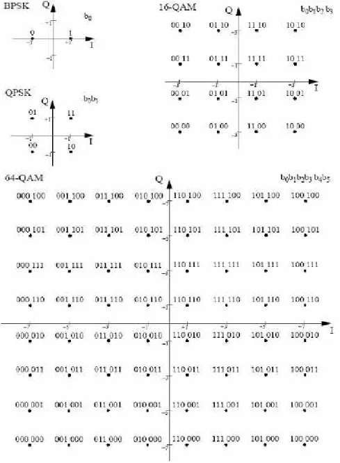
The encoded and interleaved binary serial output data shall be divided into groups of NBP SC (1, 2, 4, or 6) bits for BPSK, QPSK, 16QAM and 64QAM.
The conversion shall be performed according to Gray-coded constellation mappings, illustrated in Figure 8, with the input bit, b0, being the earliest in
the stream.
The average power for different modulation size should be normalized. The output values, d, are formed by multiplying the resulting (I+jQ) value by a normalization factor Kmod, as described in Equation 5.
d = (I + jQ) × Kmod (5)
The normalization factor, Kmod, depends on the base modulation mode,
as prescribed in Table 8 Modulation Kmod BPSK 1 QPSK √2 16QAM √10 64QAM √42 Table 3: Normalization Factor
2.5.6 OFDM modulation
In 20MHz mode, each OFDM symbol contains 64 subcarrier. There are 56 tones being used(52 data tones and 4 pilot tones). The frequency index of the data tones are -28 -22, -20 -8, -6 -1, 1 6, 8 20, 22 28, and the pilot tones are -21,-7,7,21. The 0th subcarrier is DC, the subcarrier is null. The pilot values are shown in Table 4
Table 4: Pliot Value for 20MHz
In 40MHz mode, each OFDM symbol contains 128 subcarrier. There are 114 tones is used (108 data tones and 6 pilot tones). The frequency index of the data tones are -58 -54, -52 -26, -24 -12, -10 -2, 2 10, 12 24, 26 52, 54 58, and the pilot tones are -53,-25,-11,11,25,53. The pilot values show in Table 5
2.6
Channel Model
There are six channel models, A, B, C, D, E and F, provided by TGn Sync [15] for 802.11n. The environments for these channel models can be described
Table 5: Pliot Value for 40MHz
as follows.
(Channel-A) a typical office environment, non-line-of-sight (NLOS) condi-tions, and 50 ns rms delay spread
(Channel-B) a typical large open space and office environments, NLOS con-ditions, and 100 ns rms delay spread
(Channel-C) a large open space (indoor and outdoor), NLOS conditions, and 150 ns rms delay spread
(Channel-D) the same as model C, line-of-sight (LOS) conditions, and 140 ns rms delay spread (10 dB Ricean K-factor at the first delay
(Channel-E) a typical large open space (indoor and outdoor), NLOS condi-tions, and 250 ns rms delay spread.
The time resolution of the channel model is 10ns, which is one-fifth of the sampling period (3.2ms/64=50ns). We oversample the transmitted signal by a factor of 5 and interpolate it linearly in order to convolve with the response generated by the channel model.
3
IEEE 802.11n Receiver Design
3.1
Packet Detection
Packet detection is the task of finding an approximate estimate of the start of the preamble for an incoming packet. The structure of L-LTF preamble enables the receivers to use a very simple and efficient algorithm to detect the packet. The algorithm we used is called the delay and correlate algorithm. The method is illustrated in Figure 9, which shows the signal flow structure of the delay and correlation algorithm. We define three parameter:
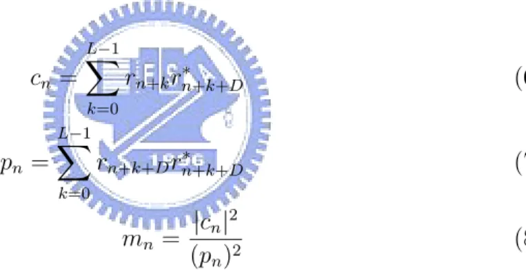
cn= L−1 X k=0 rn+kr∗n+k+D (6) pn= L−1 X k=0 rn+k+Dr∗n+k+D (7) mn= |cn|2 (pn)2 (8) The figure shows two sliding windows C and P. The window C is used to calculate the crosscorrelation between the received signal and a delay version of received signal. The delay z−D is equal to the period of the preamble.
In IEEE 802.11n, the delay D is 16. The window P is used to calculate the received signal energy. The value of the P window is then used to normalize
Figure 10: Process of Packet Detection
the decision statistic, so that it is not dependent on absolute received power level.
The variable mn is restricted between the range of [0,1]. If the received
signal only consists of noise, the output cn of the delayed crosscorrelation is
a zero-mean random variable. Once a packet is received, cn corresponds to
a crosscorrelation of two identical preambles. Thus, mn jumps up quickly to
its maximum value. Figure 10 shows the operation of the algorithm.
The approach outlined above is useful for high to normal SNR. Unfor-tunately, for low SNR, the decision statistic mn may exceed the threshold
even no packet is present. Thus, the probability of the false alarm will be increased. We can increase the threshold level; however, the probability of missing will be increased also. Here, we propose a modification to solve this problem. We add an extra window to accumulate the decision statistic. If most decision statistics (may be three forth) in the window are higher than the threshold, we then declare the detection of a packet. The rationale for this approach is that if a packet actually arrives, the decision statistics mn
will remain high until the end of preamble. Simulations show that the mod-ified approach can have more robust detection performance.
3.2
Frequency Synchronization
Both the transmitter and the receiver use their own oscillators to generate carrier and sampling signals. Unfortunately, the signal generated from the oscillator in the receiver will never have the same frequency as that from the transmitter. The difference between the transmitter and receiver oscillator frequencies is called frequency offset. The frequency offset can be divided into two types: The carrier frequency and sampling frequency offsets.
One of the main drawbacks of OFDM is its sensitivity to carrier frequency offset. The degradation is caused by two main phenomena: reduction of amplitude of desired subcarrier and ICI caused by neighboring carriers. The amplitude loss occurs because the desired subcarrier is no longer sampled at the peak of the sinc-function of DFT.
Defined the baseband transmitted signal is sn. The complex bandpass
signal yn can be expressed as:
yn= snej2πftxnTs (9)
where ftx is the transmitter carrier frequency, Ts is sampling period. The
receiver downconverts the signal with the carrier frequency frx. If we ignore
the noise for the moment, the received complex baseband signal rn will be
yn = snej2πftxnTsej2πfrxnTs
= snej2π(ftx−frx)nTs
= snej2π(Mf )nTs (10)
Many algorithms have been developed to estimate the CFO in OFDM systems. We use a data-aided scheme operating on the received time domain
Figure 11: Preamble for CFO Estimation
signal. The preamble is at least two consecutive repeated symbols. Let D be the delay between the identical samples of the two repeated symbols and define an intermediate variable z as
z = L−1 X n=0 rnrn+D∗ = L−1 X n=0 snej2πftxnTs(sn+Dej2πftx(n+D)Ts)∗ = L−1 X n=0 (sns∗n+D)(ej2πftxnTse−j2πftx(n+D)Ts) = e−j2pi(Mf )DTs L−1 X n=0 |sn|2 (11)
Equation (11) is a sum of complex variables with an angle proportional to the frequency offset. Then, the frequency offset can be estimated as:
M f = − 1 2πDTs
]z (12)
where the ]z takes the angle of its argument.
In 802.11n system, we use short preambles for coarse CFO estimate, and long preambles for fine CFO estimate. Figure 11 shows this approach.
A limitation of the CFO estimation method is its operation range, which defines how large the CFO can be estimated. The range is directly related
to the length of the repeated symbols(D). The angle of z is of the form −2π(M f )DTs, which is unambiguously defined only in the range [−π, π).
Thus the absolute value of the CFO must be lager than the limit shown below. | M f | ≤ π 2πDTS = 1 2DTs (13) For short training symbol, the sample time Ts is 50ns, and the length of
the repeated symbols is 16. Thus, the maximum frequency error that can be estimated is 625kHz. This should be compared with the maximum possible frequency error in the 802.11n system. The transmitter center frequency tol-erance shall be 20 ppm maximum for the 5GHz band and 25 ppm maximum for the 2.4GHz band. If the transmitter and receiver clocks have the maxi-mum allowed error, but with opposite signs. The total amounts of frequency error is 200kHz for the 5GHz band and 120kHz for the 2.4GHz band. The maximum frequency offset is well within the range of the estimation.
3.3
Symbol Timing Offset
The objective of symbol timing offset (STO) estimation is to locate the edge of an OFDM symbol. The result is used to define the DFT window, a set of samples for the DFT operation. Since the preamble is available to the receiver, it enables the receiver to use the simple correlation-based STO al-gorithm. After the packet is detected, the start of the packet is roughly located. The STO refines the precision to the sample-level. Thus, the packet detection can be regarded as a coarse symbol timing synchronization, and
Figure 12: Preamble for Symbol Timing
the symbol timing correction as a fine symbol timing synchronization. The refinement is performed by calculating the crosscorrelation of the received signal rn and a known reference tk.
ˆ ts = arg max | L−1 X k=0 rn+kt∗k|2 (14)
Where L is the length of reference. We select the end of short training symbol and the cyclic prefix of long training symbol as the reference signal, shown in Figure 14. The value of n that corresponds to maximum absolute value of the crosscorrelation is the symbol timing estimate. Thus, L equals 48 here.
3.4
Channel Estimation
The channel estimation is the task of estimating the frequency response of the channel. Since we generally assume that the channel response in wire-less LAN system is quasistationary, the channel response does not change during one packet. Therefore, we only need to estimate the channel once in one packet. We use the HT-LTF training symbol to estimate the channel response.
After DFT processing, the time-domain receive signal will be transformed to the frequency domain. The frequency domain received preamble for the
k-th subcarrier can be expressed (without noise) as yk = Hk x1 x2 ... xNt (15)
Where Hk is a Nr× Nt MIMO channel response matrix we want to
esti-mate, and x1, x2· · · xNt are corresponding preamble in k-th subcarrier. The
channel matrix contains Nr×Ntelements, but we only have Nr equations. ??
Therefore, we need to collect more equations in different time. Review the time-space mapping matrix and depend the number of transmitted antenna, we can generate (14) to the equations below:
When two transmitted antennas are used, the equations can be incrased as [yk(n), yk(n + 1)] = Hk · x1 −x1 x2 x2 ¸ (16) [yk(n), yk(n + 1)] · x1 −x1 x2 x2 ¸T = Hk · x1 −x1 x2 x2 ¸ · x1 −x1 x2 x2 ¸T (17) Since x1, x2 = ±1, we then have
[yk(n), yk(n + 1)] · x1 −x1 x2 x2 ¸T = Hk · 2 0 0 2 ¸ = 2Hk (18) Thus, Hk= 1/2 × [yk(n), yk(n + 1)] · x1 −x1 x2 x2 ¸T (19) Use the same method in three and four transmitted antennas. We can have the channel estimation result as
Hk = 1/4 × [yk(n), yk(n + 1), yk(n + 2), yk(n + 3)] xx12 −xx21 −xx12 xx12 x3 x3 x3 −x3 T (20)
and Hk = 1/4 × [yk(n), yk(n + 1), yk(n + 2), yk(n + 3)] x1 −x1 x1 x1 x2 x2 −x2 x2 x3 x3 x3 −x3 −x4 x4 x4 x4 T (21)
3.5
Phase Tracking
Frequency synchronization is not a perfect process, so there is always some residual frequency error. The residual frequency offset will cause constellation rotation, affecting signal detection. Here, we use the data-aided method to eliminate the residual frequency error. In 802.11n, there are four pilot subcarriers in 20 MHz bandwidth mode, and eight pilot subcarriers in 40 MHz bandwidth mode. Using the known pilot subcarrier and the estimated channel, we can reestablish the received data of n-th received antenna in k-th subcarrier yk
n without phase shift as
ykn=Hˆkn,mΨkm (22) where Hˆkn,m is the estimated channel matrix in k-th subcarrier for the path from m-th transmit antenna to n-th receive antenna, and P sik
m is the pilot
value of m-th transmit antenna in k-th subcarrier.
Then, we can find the phase error by the difference of the phase between received data Rk
n and Ynk
ˆ
φ = ][Rnk(Ynk)∗] (23) After calculating the phase error of all pilot tones in one OFDM symbol, we take average of these phase, and then subtract it from the phase of the receive signal in each tone.
3.6
Sampling Frequency Offset
The sampling frequency offset (SFO) results from the mismatch between the frequency of the digital to analog converter (DAC) at the transmitter, and that of the analog to digital converter (ADC) at the receiver. The SFO will have two main effects: (1) a slow drift of the symbol timing boundary, which rotates the phase of the subcarriers similar to the timing offset, and (2) a loss of the orthogonality of the subcarriers. This is due to the subcarriers are not sampled at the optimum positions and ICI occurs. This will also result in a loss of signal to noise ratio (SNR).
The sampling error is defined as
t∆ = Trx− Ttx
Ttx
(24) where Trxand Ttxare the transmitter and receiver sampling periods. The
overall effect, after DFT, on the received subcarrier Rl,k is shown as
Rl,k = ej2πkt∆l
Ts
Tuxl,ksinc(πkt∆)Hl,k+ Wl,k+ Ct
∆ (25)
where l is the OFDM symbol index, k is the subcarrier index, Ts is the
duration of the total symbol, Tu is the duration of the useful data portion,
Wl,k is additive white noise and Ct∆ is the induced ICI due to the SFO.
Since the sampling error t∆ is very small, the ICI term can be ignored.
The remained item is ej2πkt∆lTsTu. This term shows the amount of rotation
angle experienced by the different subcarrier. Even though the term t∆ is
quite small, as l increases, the rotation may eventually become so large that correct demodulation is no longer possible. Therefore, it is necessary to compensate for the error.
The receiver only uses one oscillator to generate the carrier frequency and sampling frequency. Thus, we can find sampling frequency error using the estimated carrier frequency offset.
SF O CF O = fs fc (26) t∆= 1 fs − 1 fs+ SF O (27)
4
MIMO Detector
4.1
Problem Definition
We first consider a flat-fading MIMO system with NT transmit and NR
re-ceive antennas. The complex baseband rere-ceived vector, defined by yc = [y1, y2, . . . , yNR]
T, is given by:
yc= Hcxc+ w (28)
where xc = [x1, x2, . . . , xNT]
T is the x
i transmitted signal vector , Hc is a
NT × NR complex channel matrix, and w = [w1, w2, . . . , wNR]T is a i.i.d.
complex Gaussian noise vector. Here, we assume that each element in xc is
a quadrature amplitude modulation (QAM) signal.
The complex system model can converted to an equivalent real-valued model by separating a complex signal to the real and image parts. Thus, (??) can be rewritten as y=Hx+w (29) where y = [Re{yc} Im{yc}]T (30) x = [Re{xc} Im{xc}]T (31) H = · Re{Hc} −Im{Hc} Im{Hc} Re{Hc} ¸ (32) We will use the representation shown (29) in the following derivation. For simplicity, we define 2NT = 2NR= N.
4.2
Maximum Likelihood Detector
The optimum detector for a MIMO system is Maximum Likelihood (ML) detector. For a received vector y, and the known channel matrix H, the ML detector finds the transmitted vector x minimizing the distance from y to Hx, i.e.,:
ˆ
xM L = arg min
x∈Ψky − Hxk
2 (33)
where the set Ψ indicates all possible transmit vectors. The ML detector needs an exhaustive search over the entire set of Ψ. Let the QAM con-stellation size be M. For the number of transmitted bit streams being N, the computational complexity of ML detector is on the order of O(MN).
When M is large, the computational complexity of the ML detector be-comes prohibited. Thus, many alternatives have been proposed to reduce the computational complexity. The most well-known one may be the Sphere Decoding(SD) algorithm.
4.3
Sphere Decoding
The main idea of sphere decoding is to search a subset of Ψ, which satisfies ky − Hxk2 < r2 (34) If r is small, the required computational complexity will be effectively re-duced. Using QR-decomposition, we can have H = QR, where Q is or-thonormal matrix and R is a upper triangle matrix. Also,
R = r1,1 r1,2 · · · r1,N 0 r2,2 · · · r2,N ... 0 . .. ... 0 · · · 0 rN,N (35)
Using the result, we can rewrite (34) as
ky − Hxk2 = ky − QRxk2 = kQTy − Rxk2 = ky0− Rxk2 < r2 (36) Where y0 = QTy. Let the ith component of y0 be y0
i and that of x be xi.
Using the upper triangle structure of R, we can further decompose (36) as ky − Hxk2 = n X p=1 (yl0− n X m=p rm,pxm)2 = (y0 N − rN,NxN)2 + (y0 N −1− rN −1,NxN − rN −1,N −1xN −1)2+ . . . < r2 (37)
As we can see, the first summation term in (37) only depends on xN, the
second on xN and xN −1, and so on. Thus, (37) can form a tree search
structure of xi, i = N, N − 1, . . . , 1. The first-level of (34) can then be
written as
(y0
N − rN,NxN)2 < r2 (38)
We can find all possible xN’s satisfying (38). Then, for each candidate of
xN, we can find all xN −1’s satisfying the constraint (see (37)). Continue this
process, we can find all candidates of xN. . . x1. Thus, we only search possible
transmitted vectors, x, inside the sphere and output the one minimizing the distance between y and Hx.
In the representation (36), we can see that the radius r is a very critical parameter. If the radius is too large, there will be many candidates, and the computational complexity will be high. On the other hand, if the radius is too small, there may be no candidates can be found in certain level. In [9],
a method to find a proper radius is suggested. The radius can be chosen as: r2 = C × |det(H)|(1/N) (39) Where C is a constant, H is channel matrix.
Equation (36) can not guarantee that the number of candidates inside the sphere is non-zero. When no candidates can be found, we can either enlarge the radius and conduct the tree structure again (until at least one candi-date is found), or randomly choose a candicandi-date as the output. Apparently, the former approach will have better result. However, the computational complexity will be higher.
Although the SD algorithm requires lower computational complexity than the ML detector, it has other problems. From the algorithm described above, it is easy to see that the number of candidates inside the sphere can have large variation. It depends on the channel, the noise level, and the radius r. To have a better idea of this problem, we conduct simulations for the LSD algorithm using a 4×4 system with 64-QAM transmission. We set the radius as r2 = 8×|det(H)|(1/4), and have 10000 runs. Figure 13 shows the histogram
of the number of candidates in the SD algorithm. From the histogram, we can see that the number of candidates inside the sphere has a large variation, though the averaged number is not particularly high. This is property is not desirable in hardware implementation. Other problems include the large latency (due to the tree structure), and the difficulty in determination of the radius (even with (39)). Here, we propose a new algorithm to overcome the problems.
0 20 40 60 80 100 120 0 500 1000 1500 2000 2500 Number of Candidate
Figure 13: Histogram of Number of Candidates
4.4
Proposed Method
Recall that the ML detection uses a exhausted search for all dimensions, the complexity is then O(MN). The main idea of the proposed algorithm
is that we only conduct exhaustive search in a small number of dimensions (maybe one or two dimension), and conduct optimum estimation in rest of the dimensions. As a result, the required computational complexity is only O(M) or O(M2).
For purpose of illustration, we first use a 2 × 2 4-PAM (real) system as an example. Let the channel matrix be H and the receive signal vector be x = [x1 x2]T. The constellation of the receive signal, excluding noise, is Hx,
parallel lines in the constellation plot, corresponding to x1 = {−3, −1, 1, 3}.
Thus, to estimate x2 for a given x1, we can project the received vector y
onto the corresponding line. In this case, we then have four candidate sets of {x1, x2}. We can then choose the one with the smallest ky − Hxk2 as the
output. Figure 14 shows the idea of the proposed algorithm.
-20 -15 -10 -5 0 5 10 15 20 -15 -10 -5 0 5 10 15 x1=-3 x1=-1 x1=1 x1=3
Figure 14: Projection in each group
We now generalize the idea to a N × N MIMO system. Recall our system model in (29), the channel matrix is H = [h1, h2, . . . , hN]. The transmitted
vector is x = [x1 x2. . . xN]T, where xi is a PAM symbol. The possible values
of a PAM symbol is SP AM = {−(M − 1), −(M − 3), . . . , M − 1}, where M
is the size of PAM signal constellation. We can rewrite the system model as y = h1x1+ h2x2+ . . . + hNxN + w (40)
Let xp = sk, where sk = −(M − 1) + 2(k − 1) and k = 1, 2, . . . , M. We can rewrite (46) as y = h|1x1+ . . . + hp{zsk+ . . . + hNxN} N terms +w y − hpsk = h|1x1+ . . . + h{z NxN} N −1terms +w ˜ yk p = ˜H˜xkp + w (41) where ˜yk p = y−hpsk, ˜Hp = [h1, · · · , hp−1, hp+1, · · · , hN], and ˜xp = [x1, · · · , xp−1, xp+1, · · · , xN]T.
Now, we can project ˜ykp onto the subspace spanned by ˜Hp, and then
quantize the result to obtain a estimated symbol in the constellation (cor-responding to xp = sk). Note that the project can be conducted with the
least-squares (LS) method. Let ˇxk
p = [ˇxk1, · · · , ˇxkp−1, ˇxkp+1, · · · , ˇx (k)
N ]T be the
quantized vector of the projection of ˜yp. Then, we have ˇ xk p = Quan{( ˜H T pH˜p)−1H˜p T ˜ yk p} (42)
where the operation Quan{·} indicates the quantization operations, assigning a vector to the nearest constellation point. Note that the vector in (42) is of dimension N − 1. Denote the complelte N-dimensional vector as vk
p. Then,
vk
p = [ˇxk1, · · · , ˇxkp−1, sk, ˇxkp+1, · · · , ˇxkN] (43)
Thus, vk
p is a candidate for the ML solution. We can then repeat the process
for all k’s and obtain a set of candidates {vs1
p , · · · , vspM}. Choose the one
with the minimum distance and obtain the best exhausted-search solution in the direction of xp. Now, we can now search L different dimensions to
have better result where L ≤ N. The computational complexity will then be O(LM). The higher L indicates the higher computational complexity, but the better performance. Thus, L can be chosen as a compromise between the performance and the computational complexity.
The result derived above can now be expressed as: ˆ x = arg min x=vk p ky − Hxk2, (k = 1, 2, · · · , M ); (44) (p = p1, p2, · · · , pL), pi ∈ {1, 2, . . . , N}, pq 6= pj) (45)
The scheme proposed above can be generalized such that the exhausted search can be conducted in D directions (dimensions) where D = 1, 2, . . . , N. In other words, MDprojections have to be conducted in the chosen directions.
If D = 1, this is the algorithm we described above. If D = N, it will be equivalent to the ML detector. For the systems we considered here, we found that D = 2 will approach the ML solution very well. For each projection, we can choose fixed values from any two dimensions {xp = sk, xq = sj} where
p 6= q. Then, y = h|1x1+ · · · + hpsk+ · · · + h{z qsj+ · · · + hNxN} N terms +w y − hpsk− hqsj = h|1x1+ . . . + h{z NxN} N −2terms +w ˜ yk,jp,q = ˜Hp,qxp,q+ w (46) where ˜yk,j
p,q = y − hpsk− hqsj, and ˜Hp,q is a matrix consisting of columns of
˜
H with ˜hp and ˜hp removed, and xp,q is a vector consisting of elements of x
with xp and xq removed. Let ˇxk,jp,q be the quantized vector of the projection
of xp,q. Using the similar method in (42), we can find ˇxk,jp,q as
ˇ
xk,jp,q = Quan{( ˜HTp,qH˜p,q)−1H˜ T
Then, let ˇxk,j
p,q = [ˇxk,j1 , · · · , ˇxk,jN ] and
vk,jp,q = [ˇxk,j1 , · · · , sk, · · · , sj, · · · , ˇxk,jN ]. (48)
We can see that vk,j
p,q is a candidate for the ML solution. Now, we can choose
L combinations of (p, q) to conduct the exhausted search. In other words, we conduct L exhausted search in D dimensions. The computational complexity will be O(LM2). Finally, we can choose one vector minimizing the distance
from y to Hx, i.e, ˆ
x = arg min x=vk,jp,q
ky − Hxk2, (k, j = 1, 2, · · · , M ; (p, q) = L combinations) (49) Note that (p, q) has N(N −1)/2 combinations. As we can see, we only have to use a small L and the result can approach the ML solution very well. The choice of the combinations does not have a specific rule. From simulations, we found that if (p, q) can be chosen such that xp and xq correspond to the
real and complex component of a symbol, good performance can be achieved.
4.5
Complexity Analysis
In this paragraph, we will compare the computational complexity for the algorithms considered. Here, we only consider the number of multiplica-tions used. For a Nt× Nt MIMO system with M2-QAM transmission, the
ML detector requires (2Nt2+ 3Nt) × M2Nt multiplications in the evaluation
of (33). The proposed algorithm requires (4N2
t − 2Nt· D) × 2DL
multipli-cations in (42), and (2Nt2 + 3Nt) × MDL multiplications in (44). There
is a matrix inverse operation in (42). However note that the matrix does not have to be recomputed when a new exhausted search is initiated. The
matrix differs from its previous one only be D columns, and some fast al-gorithm has been proposed to reduce the computational complexity of the inversion. We can use the fast algorithm proposed in [10], which requires 24N3
t + 12Nt2 × L multiplications. Thus, the proposed algorithm requires
(6N2
t + 3Nt− 2NtD)MDL + 4Nt3+ 12Nt2× L multiplications in total.
Com-plexity comparison for the 2 × 2, 3 × 3 and 4 × 4 with the 64-QAM is shown in the Table 6. As we can see, the proposed algorithm has a remarkable reduction in computational complexity.
Since the throughput of the SD algorithm is variable, it is very difficult to evaluate its computational complexity analytically. Thus, we use the com-puter simulation to actually count how many multiplications are conducted for each run. We simulate SD for 10000 runs, and find the averaged and top one percent averaged results.
Table 7 shows the complexity comparison of the SD and the proposed al-gorithm. The computational complexities of the proposed algorithm shown are maximum ones in (6). From the table, we can see that the computa-tional complexity of the proposed algorithm is still much lower than the SD algorithm.
Note that the result show in Table 7 for the SD algorithm is an averaged result. It is highly possible that in some cases, the candidates in the radius is very large, and in others is very small. This property makes efficient hardware implementation difficult. The other advantage of the proposed algorithm is that it allows a tradeoff between the complexity and performance. When the complexity is the main concern, we can use smaller D and L. On the contrary, when the performance is the main concern, those parameters can
NT × NT D=1 D=1 D=1 D=2 D=2 D=2 ML
(N = 2NT) L=1 L=N/2 L=N L=1 L=2 L=4
2 × 2 248 432 800 1,040 - - 57,344 3 × 3 600 1,368 2,520 2,148 4,080 - 7.07 × 10⁶
4 × 4 1,168 3,136 5,760 3,712 6,912 13,312 7.38 × 10⁸
Table 6: Number of Multiplications required in proposed and ML algorithm NT × NT Proposed Method SD SD
(N = 2NT) (maximum) (averaged) (top 1 % averaged)
2 × 2 1,040 1,015 2,853 3 × 3 4,080 3,602 9,599 4 × 4 13,312 13,683 33,340
Table 7: Number of Multiplications required in proposed and SD algorithm
be enlarged.
4.6
Simulations
In the section, we report simulation results demonstrating the performance of the proposed algorithm. We consider the 2 × 2, 3 × 3 and 4 × 4 MIMO systems with 16-QAM and 64-QAM transmission. The channel is a Rayleigh flat-fading channel. The bit error rate (BER) is used as the performance measure. Three algorithms are compared, namely, the ML, SD and proposed algorithms. The radius of the SD method is set as 8 × |det(H)|(1/N ).
Figure 15-20 show the results for 2 × 2, 3 × 3 and 4 × 4 MIMO systems with 16-QAM modulation. From Figure 15 and 16, we can see that for 2 × 2 systems, the performance of the proposed algorithm with D=1 and L=4 is worse than that of the ML detector. When D=2 and L=1, the performance of the proposed algorithm is almost as good as that of the ML algorithm. From Figure 17 and 18, we can see that for 3 × 3 systems, the performance of
proposed algorithm with D=1 and L=6 is worse than that of the ML detector. However, it can achieve the ML bound when D=2 and L=2. Figure 19 and 20 shows the result for 4 × 4 systems. As we can see, the proposed algorithm can achieve the ML performance when D=2 and L=4.
We then evaluate the performance of the proposed algorithm in 64-QAM transmission. Figure 21 and 22 show the simulation results for 2 × 2 systems. As we can see, the performance of the proposed algorithm with D=2 and L=1 can achieve the same performance as the ML detector. Also, with D=1 and L=4, the performance is also very close to that of the ML detector. Figure 23 and 24 show the simulation results for the 3 × 3 systems. From Figure 23, we can see that the performance of our algorithm with D=1 and L=6 has a small deviation from that of the ML detector. From Figure 24, we see that when D=2 and L=2, the proposed algorithm performs the same as that of the ML detector. Finally, Figure 25 and 26 show the result for 4 × 4 systems. As we can see, when D=1 and L=8, the proposed algorithm is worse than that of the ML detector. However, it can achieve ML performance when D=2 and L=4. Note that in all cases, the SD algorithm can have almost the same performance as that of the ML detector. Note that the price to pay is a higher computational complexity since a larger radius has to be used.
Compare the simulation results for 16-QAM and 64-QAM transmission. We can find that the proposed algorithm can have more advantages when a high QAM size is used.
18 20 22 24 26 28 10−4 10−3 10−2 10−1 SNR BER SD ML D=1,L=1 D=1,L=2 D=1,L=4
Figure 15: BER comparison for 2 × 2 16-QAM(I)
18 20 22 24 26 28 10−4 10−3 10−2 10−1 SNR BER SD ML D=1,L=4 D=2,L=1
18 19 20 21 22 23 24 25 26 10−5 10−4 10−3 10−2 10−1 SNR BER SD ML D=1,L=1 D=1,L=3 D=1,L=6
Figure 17: BER comparison for 3 × 3 16-QAM(I)
18 19 20 21 22 23 24 25 26 10−5 10−4 10−3 10−2 10−1 SNR BER SD ML D=1,L=6 D=2,L=1 D=2,L=2
18 20 22 24 26 28 30 10−5 10−4 10−3 10−2 10−1 SNR BER SD ML D=1,L=1 D=1,L=4 D=1,L=8
Figure 19: BER comparison for 4 × 4 16-QAM(I)
18 20 22 24 26 28 30 10−5 10−4 10−3 10−2 10−1 SNR BER SD ML D=1,L=8 D=2,L=1 D=2,L=2 D=2,L=4
22 23 24 25 26 27 28 29 30 10−3 10−2 10−1 SNR BER SD ML D=1,L=1 D=1,L=2 D=1,L=4
Figure 21: BER comparison for 2 × 2 64-QAM(I)
22 23 24 25 26 27 28 29 30 10−3 10−2 10−1 SNR BER SD ML D=1,L=4 D=2,L=1
22 23 24 25 26 27 28 29 30 10−4 10−3 10−2 10−1 SNR BER SD ML D=1,L=1 D=1,L=3 D=1,L=6
Figure 23: BER comparison for 3 × 3 64-QAM(I)
22 23 24 25 26 27 28 29 30 10−4 10−3 10−2 10−1 SNR BER SD ML D=1,L=6 D=2,L=1 D=2,L=2
22 23 24 25 26 27 28 29 30 10−4 10−3 10−2 10−1 SNR BER SD ML D=1,L=1 D=1,L=4 D=1,L=8
Figure 25: BER comparison for 4 × 4 64-QAM(I)
22 23 24 25 26 27 28 29 30 10−4 10−3 10−2 10−1 SNR BER SD ML D=1,L=8 D=2,L=1 D=2,L=2 D=2,L=4
5
MIMO Soft Bit Demapping
5.1
Bit-interleaved Coded Modulation
Originally proposed by Zehavi [8], BICM inserts a bit-level interleaver be-tween the encoder and modulator. With this operation, bursty bit errors can be reduced, and the correction capability of the decoder can be en-hanced. As a result, BICM is suited to the fast fading channel environment. For non-fading frequency-selective channels, BICM can be cooperated with OFDM to have frequency diversity gain. Besides, when the MIMO structure is added, spatial diversity can be achieved as well. Conventional, it uses a MMSE equalizer to suppress the interference arising in the MIMO system, and then transfer the MIMO system into multiple SISO systems. Then, it applies one-dimensional soft-bit demappers obtaining soft-bit information for the received signal.
5.2
Log Likelihood Ratio
Due to use of BICM system, we have to demap a QAM symbol to its corre-sponding bits before decoding. The operation is called bit demapping. There are two kind of bits can be dempped: hard and soft bits. Hard bits are the detected bits being equals to “0” or “1”. Soft bits corresponds to proba-bilities of being equal to “0” or “1”. It is well know that soft bits in the BICM scheme can have much better performance. The computation of soft bit demapping in the SISO systems is low. In the MIMO systems; however, its computational complexity is very high, comparable to the ML detector. In this section, we will extend the algorithm proposed in the previous section
to overcome the problem. In soft demapping, Log-Likelihood Ratio(LLR) is generally used instead of probability to represent the soft information. Let y be the received signal vector, bn,k be the kth bit of its nth component, and
x be the transmit signal vector. The LLR of bit bn,k is defined as
LLR(bn,k) = ln P [bn,k = 1|y] P [bn,k = 0|y] = ln P c1∈Sn,k(1) P [x = c1|y] P c0∈Sn,k(0) P [x = c0|y] (50) where Sn,k(1) denotes the set comprising all the symbols with bn,k = 1, and so
does Sn,k(0).
Applying Bayes rule and assuming the transmit symbols being equally probable, we can have (50) as
LLR(bn,k) = ln P c1∈Sn,k(1) P [y|x = c1] P c0∈Sn,k(0) P [y|x = c0] (51) Since the noise is Gaussin, each term in the summation of (51) has an exponential form. This can be simplified by the log-sum approximation. Thus,
LLR(bn,k) = ln
maxc1∈Sn,k(1)P [y|x = c1]
maxc0∈Sn,k(0)P [y|x = c0]
(52) From Gaussian distribution, we have the conditional PDF P (x|y) as
P (X|Y ) ∝ exp(− 1
2σ2ky-Hxk
2) (53)
Using (53) in (52), we can obtain LLR(bn,k) = { min x∈Sn,k(1) ky-Hxk2− min x∈Sn,k(0) ky-Hxk2} × 1 2σ2 (54)
With the QAM mapper, we can derive two sets, Sn,k(1) and Sn,k(0), and find one symbol minimizing the distance from y to Hx in each set. The difference of the two distances is the LLR we desire. The term 1
2σ2 can be considered as
a weighting factor. If the variance of noise is low, the weighting of the LLR is high. That means this LLR is reliable, and vice versa.
5.3
List Sphere Decoding
In previous section, we review the sphere decoding algorithm. Sphere decod-ing is a detection algorithm used to reduce the computational complexity of the ML detector. We can use similar idea of sphere decoding and extend it to conduct soft bit demapping. The algorithm is called list sphere de-coding (LSD), and described below. First, reserve all the symbols lie inside the sphere ky-Hxk2 < r2, yielding a candidate list. Then, separate these
candidates into two sets, one with bn,k = 1 and the other bn,k = 0. Finally,
find the one minimizing the distance from y to Hx in each set, and take the difference of the two distances to obtain the LLR. This LSD does not increase the computational complexity of the original SD algorithm too much. The LSD inherent the variable throughput problem associated with the SD. In addition, the LSD induce another problem that it cannot guarantee at least one symbol in each set. That is to say, it is possible that one of the sets is empty. A suboptimum approach is to give an extreme value to represent the LLR of the bit. If we want to avoid the case, we must enlarge the radius and raise the number of candidate. The computational complexity will be increased also. This is a performance-complexity trade-off.
5.4
Soft Output of Proposed Algorithm
The proposed in the previous section can also be extended to conduct soft bit demapping. As we can see, the parameter L is used to define the number of exhausted searches. When L is chosen as N
D, the search can cover all
dimensions (thought separately, not jointly). As we can see, with this setting, the proposed algorithm can achieve the ML performance for 4 × 4 systems. For 2 × 2 and 3 × 3 systems, L can be chosen as less than N
D. Thus, we
consider these two cases.
For the first case where L = N
D, all dimensions are searched. Thus, it
guarantee at least one point can be found in two sets, Sn,k(1) and Sn,k(0). With the proposed algorithm, we can have an efficient method to find LLRs. For the ease of description, we consider a Nt× Nt system (where N = 2Nt with
16-QAM transmission in a noise-free environment. The received signal can be expressed as (real-value model)
y = Hx (55)
where y = [y1 y2. . . yN]T, and x = [x1 x2. . . xN]T. For each element of x,
the possible amplitude is −3, −1, 1, 3, and the corresponding mapped bits are {00}, {01}, {11}, {10}. Recalling (43), we can have projected vectors as vk
p’s, where k = 1, 2, 3, 4, for xp. It is simple to see that for k = 1, 2, the
first bit of xp is 0, and for k = 3, 4, the first bit of xp is 1. It is equivalent
to say that two candidates are also available for bp,1 = 0 and bp,1 = 1 Define
Lk
p = ky − Hvkpk2. From (54), we can then approximate the LLR of bp,1 as
Similarly, for k = 1, 4, the second bit of xp is 0, and for k = 2, 3, the
second bit of xp is 1. Using the similar method, we can have the LLR of bp,2
as
LLR(bp,2) = min{L−3p , L3p} − min{L−1p , L1p} (57)
Similarly, we can derive the LLR corresponding to the 64-QAM system of xp: LLR(bp,1) = min{L−7n , L−5n , L−3n , L−1n } − min{L1 n, L3n, L5n, L7n} (58) LLR(bp,2) = min{L−7n , L−5n , L5n, L7n} − min{L−3n , L−1n , L1n, L3n} (59) LLR(bp,3) = min{L−7n , L−1n , L1n, L7n} − min{L−5 n , L−3n , L3n, L5n} (60)
As shown above, the soft demapping is simple in the proposed algorithm. The above approach for the LLR calculation is for D = 1. It is straightfor-ward to generalize the result for case of D = 2.
For the second case is where L < N
D, there is no symmetric property can
be explored and we can not guarantee at least one candidate can be found for Sn,k(1) and Sn,k(0). In this case, we can use the similar idea in the LSD algorithm. We can construct a candidate list with the vectors we select in (43) or (48), correspond to the case of D = 1 or D = 2. Then, we also partition these candidates into two sets, one with bn,k = 1 and the other with bn,k = 0. Then,
we can find the one minimizing the distance from y to Hx in each set, and take the difference of the two distances to obtain the LLR. Note that the size
of candidates is LM or LM2, a function of L. This is contrast to the LSD
algorithm in which the number of candidates cannot be controlled.
5.5
Simulations
In the section, we will report simulation results demonstrating the perfor-mance of the proposed algorithm. Similar to the last section, We consider 2×2, 3×3 and 4×4 MIMO systems with 16-QAM and 64-QAM transmission. The channel is again a Rayleigh flat-fading channel. A convolutional code with a constraint length of 7 is used in the transmitter, and soft decoding is conducted.
Two algorithms are compared, namely, the LSD and proposed algorithms. The radius of the LSD method is set as 8 × |det(H)|(1/N).
Figure 27-32 show the results for 16-QAM transmission. Figure 27 and 28 show the result of 2 × 2 systems. Let the target BER be 10−3. From
the figures, we can see the performance of the proposed algorithm with D=1 and L=4 is 0.5dB better than that of the LSD algorithm, and 2.5dB better than that of the LSD algorithm when D=2 and L=1. Figure 29 and 30 show the simulation result of 3 × 3 systems. When D=2 and L=1, the proposed algorithm can achieve the performance of that of the LSD algorithm. When D=2 and L=2, The performance of the proposed algorithm is 1.5 dB better than that of LSD. The result of 4 × 4 16-QAM system is shown in Figure 31 and 32. Performance of proposed algorithm with D=2 and L=1 is approx-imately the same as the of the LSD algorithm. When D=2 and L=2, the proposed algorithm outperform the LSD algorithm about 0.5 dB.
and Figure 34, we can see the result of 2 × 2 systems. When D=1 and L=2, the proposed algorithm can have the same performance as that of the LSD algorithm, and when D=2 and L=1, the proposed algorithm can outperform the LSD algorithm about 3 dB. Figure 35 and 36 show the results for 3 × 3 systems. From Figure 35, we can see when D=1 the proposed algorithm cannot better than the LSD algorithm. From Figure 36, we found that to outperform the LSD algorithm, at least the setting of D=2 and L=2 must be used. Finally, Figure 37 and 38 show the result for 4 × 4 systems. When D=2 and L=2, the proposed and LSD algorithm have the same performance. With D=2 and L=4, the proposed method outperform the LSD algorithm by 1 dB.
To realize how much performance gain we can obtain with the soft decod-ing, we conduct another set of simulations. Figure 39 and 40 show the results of hard and soft decoding, Figure 39 for a 3 ×3/64-QAM, and Figure 40 for a 4 × 4/64-QAM system. Note that in soft decoding, MIMO soft demapping is required. As we can see, in 3 × 3 systems, the gap between the LSD and SD algorithm is approximately 2.5 dB. For the proposed algorithm with D=2 and L=2, the gap is about 3.5 dB. In 4 × 4 systems, the gap of the LSD and SD algorithms is 1.5 dB, and 2.2 dB of the proposed algorithm when D=2 and L=4.
12 13 14 15 16 17 18 10−4 10−3 10−2 10−1 100 SNR BER LSD D=1,L=1 D=1,L=2 D=1,L=4
Figure 27: BER comparison of soft demapping for 2 × 2 16-QAM system(I)
12 13 14 15 16 17 18 10−5 10−4 10−3 10−2 10−1 SNR BER LSD D=1,L=4 D=2,L=1 D=2,L=2
14 15 16 17 18 19 20 21 22 10−5 10−4 10−3 10−2 10−1 100 SNR BER D=1,L=1 D=1,L=3 D=1,L=6 LSD
Figure 29: BER comparison of soft demapping for 3 × 3 16-QAM system(I)
14 15 16 17 18 19 20 21 22 10−5 10−4 10−3 10−2 10−1 SNR BER D=1,L=6 D=2,L=1 D=2,L=2 LSD