Robust State Feedback Control Through Actuators With Generalized Sector Nonlinearities And Saturation

ROBUST STATE FEEDBACK CONTROL THROUGH ACTUATORS

WITH GENERALIZED SECTOR NONLINEARITIES AND SATURATION

Chih-Chin Hsu and I-Kong Fong

ABSTRACT

In control systems, actuators often have nonlinear characteristics that can not be neglected. For linear systems driven by actuators satisfying the generalized sector condition, a robust state feedback controller synthesis method is proposed to achieve the ultimate boundedness control. The method is based on the linear matrix inequality approach and is easy to apply. As an important special case of the generalized sector condition, the saturation characteristic of actuators is discussed separately, and non-conservative re-sults are obtained.

KeyWords: Actuator nonlinearity, LMI, robust stability, saturation. I. INTRODUCTION

Most actuators in real control systems are subject to some nonlinearities due to technological factors or physical constraints. Though many actuators are manu-factured so as to have pretty good linear characteristics over their main operation ranges, nonlinearities, such as deadzone and saturation, inevitably exist. It is just a mat-ter of degree. For certain applications, especially those that involve large amounts of power, if these nonlineari- ties are not properly accounted for, they will cause the overall performance to deteriorate, damage the system, or result in instability. Consequently, for many decades, control problems with nonlinear actuators have attracted considerable interest, and no less recently [8,11,12,14, 15]. In the celebrated Lur’e problem [16], a general class of nonlinearities are described by means of the so-called sector condition, and many analytic or graphic stability criteria are derived. However, some common nonlineari- ties, such as deadzone and hysteresis, which are often seen in hydraulic or electro-magnetic devices, do not satisfy the sector condition. Therefore, we will propose a generalized sector condition to cover more nonlinear characteristics of actuators and discuss the corresponding control problem.

In addition, we will discuss a specific problem in-volving actuators with the standard saturation

character-istic. It is probably the most frequently studied problem when actuator nonlinearities are the issue because almost all actuators have this characteristic. To deal with this problem, one very important approach is to use the set invariance concept [3,20]. The main idea is to establish some positively invariant set in the state space. This ap-proach can be further divided into apap-proaches that use ellipsoidal and polyhedral invariant sets, which lead to various solution methods, depending on the adopted mathematical tools, such as linear programming [1,2,18, 19], convex optimization [6,11], eigenstructure assign-ment [5], and polynomial formulation [10]. For this input saturation problem, the goal is usually to find a stabiliz-ing controller, or to find a large stability region in the state space, given a stabilizing controller and actuator saturation data [6,12,17]. Here, we will attempt to achieve both goals by utilizing the results derived for the general nonlinearity problem.

Besides actuator nonlinearities, the other feature of the control problem studied in this paper is plant uncer-tainty. We will adopt the polytopic linear differential inclusion (PLDI) description [4] for the plant and study the robust state feedback stabilization problem. The ex-act problem formulation will be given in Section 2. A sufficient condition for the existence of an ultimate boundedness controller in the presence of actuators sat-isfying the generalized sector condition will be devel-oped in Section 3. The sufficient condition will be given in terms of a linear matrix inequality (LMI) so that it will be easy to search for feasible controllers, which will eventually regulate the system trajectories inside an el-lipsoidal ultimate boundedness set with the major semi-axis shorter than a prescribed length. In Section 4, Manuscript received March 3, 2001; revised October 9,

2001; accepted January 15, 2003.

The authors are with Department of Electrical Engineering, National Taiwan University, Taipei, Taiwan 10617, Republic of China.

we shall apply the results given in Section 3 to deal with control problems with saturating actuators and look for state feedback gain and a stability region simultaneously. Here, all the results involve LMI or bilinear matrix ine-quality (BMI) and will be accompanied by examples to show how the proposed methods can be applied. Finally, some conclusions will be drawn in Section 5.

Before we start, we will define some notations first. For any two matrices X, Y ∈ Rn×n_{, X ≥ Y means that X, Y}

are symmetric, and that X – Y is positive semi-definite. Similar notations will apply to symmetric positive/nega- tive definite matrices. If X > 0, then λmax(X) denotes its

largest eigenvalue. The notation diag(X1, …, XA) stands

for the block diagonal matrix with diagonal blocks X1, …,

XA. The transpose of a real matrix X is denoted by XT. Im

is the m × m identity matrix, and ei is the ith column of Im.

In a symmetric block matrix, for simplicity, the symbol * represents the submatrices that lie above the diagonal. Finally, the notation ⋅ denotes the 2-norm of the ar-gument vector or matrix, and Co{⋅} represents the con-vex hull of the set in the argument.

II. PROBLEM FORMULATION

Consider the uncertain system described by the mathematical model 0 1 1 ( ) ( ) ( ) ( ) ( ), (0) , ( ) ( ), ( ) [ ( , ( )) ( , ( ))] ,T m m x t A t x t B t u t x x u t Kx t u t ψ t u t ψ t u t = + = = = (1) where 1 1 [ ( ) ( )] Co{[A t B t ∈ A B], , [A Bl l]}. (2) The first equation in (1) represents a plant descibed by

PLDI with the state vector x(t) ∈ Rn _{and the input vector}

u(t) = [u1(t) … um(t)]T∈ Rm. It is assumed that the pairs

{Ai, Bi}, i = 1, 2, …, l, are controllable. The plant is to

be stabilized by the state feedback controller of the sec-ond equation in (1), where ũ(t) = [ũ1(t) … ũm(t)]T∈ Rm

is the control signal vector, and K = [ 1

T T

m

k …k ]T_{∈ R}m×n

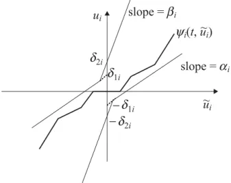
is the state feedback gain matrix. The third equation in (1) represents m actuators which convert the control signals to inputs. The jth actuator is assumed to have the nonlinear characteristic ψj(⋅, ⋅) : [0, ∞) × R → R, which

belongs to the generalized sector [αj, βj] with bias [δ1j,

δ2j], as shown in Fig. 1. Note that the actuator nonlinear

characteristic is not confined in the first and third quad-rants, and does not necessarily pass the origin of the characteristic plane. This enables us to accommodate many of actuator nonlinearities, especially those which are multi-valued, such as backlash, and do not belong to the standard sector condition [16]. Mathematically, this

2i

−

−

u

u

~

~

Fig. 1. Generalized sector nonlinearity.

is equivalent to saying that at any instant t, the signals

uj(t) and k x t satisfy one of the following conditions: Tj ( )

1 2 [ ( )u tj −αjk x tj ( )+δ j][ ( )u tj −βjk x tj ( )−δ j] 0≤ (3) or 1 2 [ ( )u tj −αjk x tj ( )−δ j][ ( )u tj −βjk x tj ( )+δ j] 0≤ (4) for j = 1, …, m.

For the above system (1), we will discuss in Sec-tion 3 how to synthesize state feedback controllers to achieve the ultimate boundedness control. The following definition gives a precise description of the concept of ultimate boundedness.

Definition 1. [13] The solutions of

0 0

( ) [ , ( )], ( ) ,

x t = f t x t x t =x (5)

are ultimately bounded (with bound β) if there exists a β > 0 and if corresponding to any α > 0 and t0≥ 0, there

exists a t1(α) > 0 such that x0 < α implies that x t( )

< β for all t ≥ t0 + t1.

In this paper, the control purpose is made more specific. Given a number γo > 0, it is desired that the

state trajectories of the system (1) eventually enter and stay within some ellipsoidal set Ec = {x ∈ Rn | xTPx ≤ c},

where P > 0, c > 0, and the major semi-axis of Ec is no

longer than γo. The problem is to derive conditions which

enable us to find state feedback controllers such that the system (1) behaves as desired. In Section 4, we will fo-cus on actuators with the standard saturation characteris-tic (to be defined later). In this case, the control purpose is to make the closed-loop system asymptotically stable. However, due to saturation, not all the trajectories can be

brought back to the origin of the state space. Hence, the problem is to find a state feedback controller which forces the state trajectories that start from the largest possible ellipsoidal set P = {x ∈ Rn _{| x}T_{Px ≤ 1} of initial}

conditions to converge. Here, the concept of a positively invariant set will be called upon, and a definition for it is given below.

Definition 2. [3,20] The set Ω ⊂ Rn _{is said to be}

posi-tively invariant for the system (5) if for all x(t0) ∈ Ω, the

solution x(t) ∈ Ω for all t > t0.

III. GENERALIZED SECTOR NONLINEARITIES

We will first present an LMI-based condition for the existence of state feedback controllers which solve the problem defined in Section 2.

Theorem 1. Consider the uncertain system (1) driven by

nonlinear actuators which satisfy the generalized sector conditions depicted in Fig. 1. Let Smin = diag(α1, …, αm),

Smax = diag(β1, …, βm), δ1 = [δ11… δ1m]T, and δ2 = [δ21

… δ2m]T. For a given γo > 0, if the LMIs

2 1 1 2 1 1 1 * * * 1_{( ) ˆ} * * 2 0, 1_{( )} 1_{( )} * 2 2 0 0 i T T i max min m n B S S Y T Q I δ δ δ δ τ − − + Π      _{− −}      <  _{− + −}       −    ε i = 1, 2, …, l, (6) 1 1 2 , m o τ− λ γ + + ≤ (7) and 1 1 1 ˆ , 0, ˆ 0, 0, n n m I Q I T λ − τ− + ≥ ≥ε > ε> > (8) where 1 1 _{( )} 2 1 _{( ) ,} 2 T i i i i max min T T T T max min i i i QA A Q B S S Y Y S S B B T B− Π = + + + + + + (9)

have the feasible solutions Q _{∈ R}n×n_{, Y ∈ R}m×n_{, T}−1 _∈

Rm×m, 1 1

m

τ−

+ , λ, and ˆε , then the static state feedback

control ũ(t) = Kx(t) with K = YQ–1 _{causes the trajectories}

of the system (1) to converge to and stay within the el-lipsoid set Ec = {x ∈ Rn | xTPx ≤ c}, where P = Q–1, c =

1 1

m

τ−

+ , and γo is an upper bound of the major semi-axis

length of Ec.

Proof. For Ec = {x ∈ Rn | xTPx ≤ c} to be an ultimate

boundedness region of the controlled system (1), it is sufficient to ensure that the time derivative of the Lyapunov function candidate υ(x) = xT_{Px is negative}

along all the state trajectories of (1) outside Ec for all the

considered generalized sector nonlinearities. Here, we require that dυ[x(t)]/dt be negative outside a ball Bε = {x

∈ Rn _{| x}T_{x ≤ ε} which is contained by the set E}

c for all

the considered generalized sector nonlinearities. This is implied by the S-procedure [4], or by the existence of positive τj and τ , j = 1, …, m + 1, such that j

1 2 1 1 [ ( ) ( )] ( ) ( ) ( )( ) ( ) 0 T T T T T m j j j j j j j j j j T m x A t P PA t x x PB t u u B t Px u k x u k x x x τ α δ β δ τ = + + + + − − + − − − − <

∑

∑

for all nonzero x, u, and [A(t) B(t)] satisfying (2). Let us discuss (10) first. Defining ˆε = τm+1ε > 0 and T =

diag(τ1, …, τm), we can rewrite (10) as

1 2 1 2 1 2 1 [ ( ) ( )] ( ) ( ) ˆ 0, T T T T T T T T T T

min max min max

T T T T max min T T m x A t P PA t x x PB t u u B t Px u Tu u TS Kx u TS Kx x K S TS Kx TS Kx u T Tu TS Kx T x x δ δ δ δ δ δ τ + + + + − + + − + + − − + − +ε < (12)

which must hold for all [A(t) B(t)] ∈ Co{[A1 B1], …, [Al

Bl]. In matrix language, this is equivalent to

1 1 2 1 2 2 1 1 _ˆ ( ) ₀ 2 1 1 ( ) ( ) 2 2 T T i i m n min max T T T max min T i max min A P PA I K S TS K TS TS K T B P T S S K T T τ δ δ δ δ δ δ + + + − ∗ ∗ − − _{∗ <} + + − −                 ε (13) for i = 1, 2, …, l. By the Schur-complement [4], (13) is

1 1 1 2 2 1 2 1 1 ( ) 2 1 ( ) 2 1 ( ) ( ) 4 1 ( ) 2 1 ( ) 2 1 ( ) ( ) 4 T i i m n T T min max i i T T T min max i i min max T

min max min max

T T max min T T i T min max A P PA I K S TS K PB T B P K S S B P PB S S K K S S T S S K TS TS K B P T S S K τ δ δ δ δ δ δ + − + + − + + + ∗ + + + + + − + − + − +                                1 2 2 1 2 1 0 ˆ 1 ( ) ( ) 4 . T T T δ δ δ δ δ δ < − + − −                                         _ _      _ _   _    ε (14) Multiplying diag(P–1_{, 1) from the left and right hand}

sides to (14) and letting Q = P–1 _{> 0, Y = KQ, we obtain}

2 1 1 2 1 2 1 2 1 2 1 1 _{( )} 2 1 ( ) 2 1 ( ) ( ) 4 1_{( )} 1 2 _{ˆ ( ) ( )} 1_{( ) ( )} 4 4 T T i i m i i T T T min max i i min max T T

max min max min

T T i T T max min QA A Q Q B T B Y S S B B S S Y Y S S T S S Y B T T S S Y τ δ δ δ δ δ δ δ δ − +  + + +      _{+ +}      _∗  _{+ +}      + − −     _{ }  _ − _  _{  − + + +}  _{ }  _+ + − _  ε 0

.

with the pivot term τm+1Q2 and once with the pivot term

1 4Y

T_(S

max− Smin)TT(Smax− Smin)Y, the main inequality (6)

can be obtained. The condition Bε = {x ∈ Rn | xTx ≤ ε} ⊆

Ec = {x ∈ Rn | xTPx ≤ c} is satisfied by setting c = τm−1+1

and requiring, accordingly, Q ≥ ˆεIn > 0. In addition, the

major semi-axis length of Ec is equal to τm−1+1⋅λmax( ),Q

which will be no greater than γo provided that (7) and

the first inequality of (8) hold since 1

1 ( ) m max Q τ− λ + ⋅ ≤ 1 1 1 [ ( )] 2 τm λmax Q − + + .

As for the inequality (11), parallel derivation leads to the following equivalent condition:

2 1 1 2 1 1 1 1 ( ) 2 _0, 1_{( )} 1_{( )} 2 2 0 0 i T T i max min m n B S S Y T Q I δ δ δ δ τ − − +  Π ∗ ∗ ∗     _{− + − ∗ ∗}   _{ <}    _{− − − − ∗}     ₋    ε i = 1, 2, …, l, (16) where ε=τm+1ε and 1 1 _{( )} 2 1 ( ) . 2 T i i i i max min T T T T max min i i i QA A Q B S S Y Y S S B B T B− Π = + + + + + +

However, multiplying diag(In, −1, Im, 1) from the left and

right hand sides to (16) to get

2 1 1 2 1 1 1 1_{( )} 2 _0, 1 1 ( ) ( ) 2 2 0 0 i T T i max min m n B S S Y T Q I δ δ δ δ τ − − +  Π ∗ ∗ ∗     _{+ − ∗ ∗}   _{ <}    _{− + − ∗}     ₋    ε i = 1, 2, …, l,

quickly tells us that the conditions derived from (11) are redundant, and that we only need conditions (6), (7), and

(8). „

Remark 1. The expressions (6), (7), and (8) form an

LMI feasibility problem in the variables Q, Y, T−1, ˆε , λ,

and 1

1

m

τ−

+ , which can be solved with the help of [9] to

determine a state feedback controller ũ = Kx for the ul-timate boundedness control. Since the feasibility prob-lem may have more than one solution, solutions corre-sponding to low controller gains are usually desirable. Thus, we form the following convex optimization prob-lem:

minmize Y (17)

subject to (6), (7), and (8),

where the two-norm of Y is chosen as the objective func-tion to indirectly minimize the controller gain K = YQ−1. Though the solution may not give the smallest gain ma-trix, our numerical experience indicates that excessively large gain matrices are indeed avoided.

Remark 2. When δ1j =δ2j = 0, the generalized sector

con-dition described by (3) and (4) reduces to the standard sector condition [16] formulated by (uj− αjkjx)(uj− βjkjx)

≤ 0. In this case, the control problem discussed previously turns into that of finding state feedback controllers to en-sure asymptotic stability instead of ultimate boundedness of the closed-loop system trajectories. Results of this spe-cial case stated below will be applied to study the actuator saturation problem in the next section.

Corollary 1. Consider the polytopic uncertain system (1)

driven by nonlinear actuators which satisfy the sector conditions

(uj−αjk x uj )( j−βjk xj ) 0,≤ j= …1, , .m

If there exist a positive definite matrix Q ∈ Rn×n_{, a}

posi-tive definite matrix T−1∈ Rm×m_{, and a matrix Y ∈ R}m×n

satisfying 1 1_{( )} 0, 1, 2, , , 2 i max min i l S S Y T− Π ∗    _{− −}  < =     … (18)

then the state feedback control ũ(t) = Kx(t) with K = YQ−1

will asymptotically stabilize the closed-loop system (1). Note that Smax, Smin, and Πi are defined in Theorem 1.

Proof. It is easy to mimic the proof of Theorem 1 to

show that under the assumed conditions, we have

1 [ ( ) ( )] [ ( ) ( )] ( ) ( ) ( )( ) 0, T T T T T T m j j j j j j j j d x t Px t x A t P PA t x dt x PB t u u B t Px u k x u k x τ α β = = + + + <

_∑

where P = Q−1_{, for all nonzero x, u, and [A(t) B(t)]}

satis-fying (2). Here, we can see that in addition to the as-ymptotic stability as concluded above, it is also true that the ellipsoidal set P = {x ∈ Rn _{| x}T_{Px ≤ 1} is a positively}

invariant set [3,20] of the closed-loop system. „

We will give one example to illustrate the proposed ultimate boundedness controller synthesis approach.

Example 1. Consider the uncertain system (1) with two

states, one input, and

1 1 11 21 0 0.5 0.5 ( ) , ( ) , ( ) [ 1, 1], 0.8 ( ) 0.2 ( ) 0.8, 1.2, 0.2, 0.3. A t B t p t p t p t α β δ δ −     =_{ } =_{ } ∈ − −     = = = =

For γo = 0.5, we can solve (17) to obtain

[

]

[

]

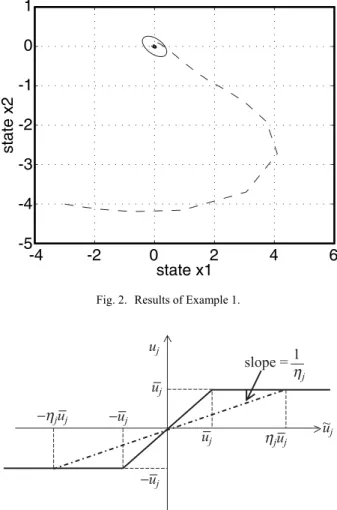
In Fig. 2, the solid ellipse is the ultimate boundedness ellipsoidal set Ec we derived. The actuator is assumed to

have the backlash characteristic with a deadband width of 0.25 for the purpose of simulation. Clearly, starting from the initial condition xo = [−3 −4]T, the state

trajec-tory (dashed line) of the closed-loop system subject to

-4 -2 0 2 4 6 1 0 -1 -2 -3 -4 -5 state x1 state x2

Fig. 2. Results of Example 1.

u_j slope = u_j ~ − u−_j −u−j −u−j − u−_j

Fig. 3. Standard saturation characteristic.

the uncertain parameter p(t) = sin(2 ) 10

π _{enters and stays} within Ec eventually.

IV. ACTUATORS WITH THE STANDARD SATURATION CHARACTERISTIC In this section, we will focus on the polytopic un-certain system (1) driven by actuators that have the standard saturation characteristic; i.e., for j = 1, …, m, and all t ≥ 0, , , ( , ) , , , . j j j j j j j u u t u u u u ζ ψ ζ ζ ζ ζ  ≥  =_ − < < − ≤ −  (19)

This characteristic is depicted in Fig. 3 using thick, solid lines.

At first sight, this particular problem can be solved by using Corollary 1 in Section 3 with Smin = 0 and Smax

= Im. However, the range of applicable cases will be

1 2 _0, 1 2 T T i i i T i A P PA PB K T B P TK T  _{+ +}   _<   + −    

which is feasible only if T i

A P+ PAi < 0 for some P > 0,

implying that all Ai, i = 1, 2, …, l, must be Hurwitz.

This reflects the fact that when unstable plants and satu-rating actuators are involved, in general, it is impossible to stabilize the entire state space. Thus, one must change the control objective. The linear part of the standard saturation characteristic suggests that any stabilizing state feedback controller for the linear plant in (1) can still stabilize some state trajectories of the closed-loop system with the saturating actuators, provided that the initial condition xo is close enough to the origin of the

state space. Thus, the goal may become that of finding state feedback controllers which can handle the largest possible set of initial conditions, from which all the state trajectories will be brought back to the origin asymptoti-cally. As a starting point, we apply Corollary 1 of Section 3 with Smin = Smax = Im in (18) but add the

con-straint that the set P = {x ∈ Rn _{| x}T_{Px ≤ 1} is inscribed}

by the set {x ∈ Rn _{| |k}

jx| ≤ ūj, j = 1, …, m}, which can be

formulated by the LMI constraints

2 0, 1, , . T j j T j u e Y j m Y e Q   ≥ =       … (20)

Clearly, the idea is to have |ũj| = |kjx| ≤ ūj, j = 1, …, m, so

that no actuators will saturate. Also, since P is a positively invariant set, it can serve as the set of stabi- lized initial conditions we are looking for. However, this still causes an unnecessary restriction since to bring the system states back to the origin, the actuators need not be unsaturated at all times.

Suppose the jth actuator is allowed to saturate at most to the level ηj≥ 1, which means that |ũj(t)| must not

exceed ηjūj for all t ≥ 0. In this situation, the nonlinearity

of the jth actuator belongs to the sector [1/ηj, 1], as can

be seen in Fig. 3. Hence, the method proposed in Section 3 can be applied again, with Smin = diag(1/η1, 1/η2, …,

1/ηm) and Smax = Im in (18). In the extra constraints (20),

the term 2

j

u should be replaced with 2 2

juj

η . The next

issue is the question of whether ηj’s are known

before-hand. Usually, for technical or safety reasons, we have an upper bound η for each ηj j but do not know how to

pre-select a set of ηj’s so that the resultant stabilized

re-gion P is as large as possible. This motivates us to ex-amine the related LMIs more closely. Now (18) is

1 1 ( ) 2 _{0, 1, 2, , ,} 1_{( )} 2 T T i m min m min Y I S i l I S Y T−  _{Π −}   _{< =}   − −     … (21) where 1 1 _{( )} 2 1 ( ) 2 T i i i i m min T T T T m min i i i QA A Q B I S Y Y I S B B T B− Π = + + + + + +

and Smin = diag(1/η1, 1/η2, …, 1/ηm). The other set of

LMIs is 2 2 0, 1, , , T j j j T j u e Y j m Y e Q η   ≥ =       … or equivalently 2 _/ 0, 1, , . / T j j j T j j u e Y j m Y e Q η η   ≥ =       … (22)

Note that (21) and (22) are LMIs with respect to the variables {Q, Y, T−1_{} as well as with respect to {Q, S}

min,

T−1_{}. Thus, they are BMIs with respect to the variables}

{Q, Y, Smin, T−1} and remain so after another set of LMIs,

, 1, 2, , ,

T T T

i i i i

A Q QA+ +B Y Y B+ <rQ i= … l (23) is augmented with a pre-assigned r < 0 to set the mini-mum trajectory decay rate when all the actuators enter their linear range.

Since the only coupled variables in the above non-convex BMIs are Y and Smin, a popularly adopted

approach is to solve them alternately. Hence, we propose the following two convex problems (CPs) for the given plant and saturation information {A(t), B(t)}, Smin =

diag(1/η , 1/1 η , …, 1/2 η ), and ūm j, j = 1, …, m: 1 1 0 , ,0 0 , ,0 CP1 min subject to (21), (22), (23), from CP2, CP2 min subject to (21), (22), (23), from CP1, n n min min m I Q Y T min min I Q S S I T S S Y Y ξ ξ ξ ξ − − < ≤ < ∗ < ≤ < ≤ < ∗ − = − =

which are to be solved altenately. Note that minimizing the objective function “−ξ ” is equivalent to maximizing the minimum eigenvalue of Q, which is proportional to the minimum semi-axis length of the ellipsoidal set P = {x ∈ Rn _{| x}T_{Px < 1}. This lets us obtain a large stability}

region. To begin, CP1 is solved first with Smin set to Im or

whatever are feasible values are deemed appropriate. To end the procedure, a stopping rule may be that the in-crement of ξ* _{becomes insignificant. Because each}

sequence of optimal ξ*_{’s will be monotonically non-de-}

creasing. However, as a whole, the sequence may con-verge to a local optimum.

Example 2. Consider the linearized equations of motion

for a satellite studied in [7] and [12], which are in the form of a polytopic uncertain system with four states and two inputs. In [7], the authors found a linear state feed-back controller that stabilized the system for any initial condition x(0) ∈ {xT_{x ≤ 1} under constrained control.}

Subsequently, in [12] it was shown that the controller from [7] could actually stabilize the system for more initial conditions, and an ellipsoidal set P which had a volume 11.30 times larger than that of the unit sphere {xT_{x ≤ 1} was shown to be a positively invariant set of}

the closed-loop system. Here, the problem is studied again to test the method proposed in this section. To let the test conditions be as close to those used in [7] and [12] as possible, Smin is set to 0 because there are no

lim-its on how saturated the actuators are allowed to be, and

r is set to −2 in (23) to match the decay rate of the closed-loop system of [7] and [12] when actuators are not saturated. We can solve CP1 and CP2 alternately from the simplest initial guess Smin = I2 until ξ converges

to a local optimum and get

10.402 4.305 3.057 0.211 , 5.664 0.465 11.067 7.293 9.267 15.576 0.518 2.462 15.576 52.338 3.676 2.644 , 0.518 3.676 5.443 6.469 2.462 2.644 6.469 35.301 K Q ∗ ∗ − − −   =   − − − −     − − −     − −   =   − −    _{− − −}   

which give us a new state feedback gain matrix and a new positively invariant set P for the initial conditions. The volume of the new set is 179.956 times larger than that of the unit sphere. It is also interesting to note that

1

η∗ _{= 1.576, not equal to} 2

η∗ _{= 2.563. Different initial}

guesses of Smin do result in different local optimal

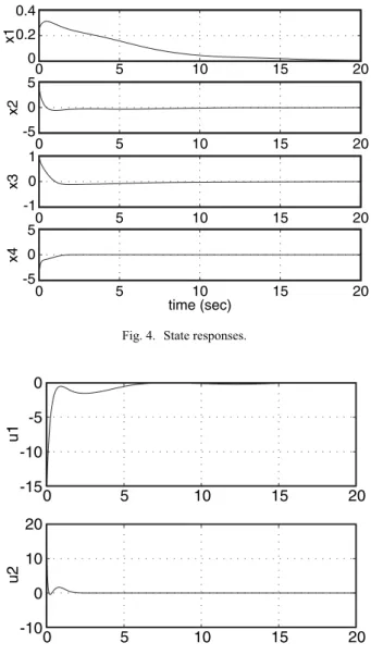
solu-tions or positively invariant sets P due to the non-con- vexity of BMIs. How to get the global optimal solution by adopting, for example, the branch and bound search method is still being studied. In Fig. 4, all the state vari-ables starting from the initial condition [0.25 4.0 1.0 −4.0]T _{are found to converge to zero. The system is}

as-sumed to be subject to a time-varying uncertain parame-ter p(t) given in [12], which lies within the inparame-terval [0.5, 1.5] and is set to 1 + 0.5 sin(2

10

π _{) for the purpose of} simulation. The two actuator outputs that drive all the system states to the origin of the state space are also plotted in Fig. 5. These outputs are limited to a saturation level of ±15. 0 5 10 15 20 0.4 0.2 0 x1 0 5 10 15 20 5 0 -5 x2 0 5 10 15 20 1 0 -1 x3 0 5 10 15 20 5 0 -5 x4 time (sec)

Fig. 4. State responses.

0 5 10 15 20 0 -5 -10 -15 u1 0 5 10 15 20 20 10 0 -10 u2

Fig. 5. Actuator output signals. 5. CONCLUSIONS

For polytopic uncertain systems with nonlinear ac-tuators which satisfy generalized sector conditions, we have derived LMI conditions to guarantee the existence of robust state feedback controllers and to achieve the ultimate boundedness control. For the case in which ac-tuators have the standard saturation characteristic, the proposed conditions can be adapted in order to find state feedback controllers that stabilize state trajectories from a large set of initial conditions. Examples have been pro-vided to illustrate how these new methods are used.

REFERENCES

1. Bitsoris, G., “On the Positive Invariance of Polyhe-dral Sets for Discrete-time Systems,” Syst. Contr.

Lett., Vol. 11, No. 3, pp. 243-248 (1988).

Regula-tion of Linear Systems,” Automatica, Vol. 31, No. 2, pp. 223-227 (1995).

3. Blanchini, F., “Set Invariance in Control,”

Auto-matica, Vol. 35, No. 11, pp. 1747-1767 (1999).

4. Boyd, S., L. El Ghaoui, E. Feron, and V. Balakrish-nan, Linear Matrix Inequalities in System and

Con-trol Theory, SIAM, Philadelphia, PA (1994).

5. Castelan, E. B. and J. C. Hennet, “On Invariant Poly-hedra of Continuous-time Linear Systems,” IEEE

Trans. Automat. Contr., Vol. 38, No. 11, pp. 1680-

1685 (1993).

6. Gomes da Silva, Jr., J. M. and S. Tarbouriech, “Lo-cal Stabilization of Discrete-time Linear Systems with Saturating Controls: an LMI-based Approach,”

Proc. Amer. Contr. Conf., Philadelphia, PA, pp.

92-96 (1998).

7. Dolphus, R. M., and W. E. Schmitendorf, “Stability Analysis for a Class of Linear Controllers Under Control Constraints,” Proc. 30th IEEE Conf. Decis.

Contr., Brighton, England, pp. 77-80 (1991).

8. Fong, I-K., and C.-C. Hsu, “State Feedback Stabili-zation of Single Input Systems through Actuators with Saturation and Deadzone Characteristics,” Proc.

39th IEEE Conf. Decis. Contr., Sydney, Australia,

pp. 3266-3271 (2000).

9. Gahinet, P., A. Nemirovski, A. J. Laub, and M. Chilali, LMI Control Toolbox, The MathWorks, Inc., Natick, MA (1995).

10. Henrion, D., S. Tarbouriech, and V. Kucera, “Con-trol of Linear Systems subject to Input Constraints: A Polynomial Approach, Part I-SISO Plants,” Proc.

38th IEEE Conf. Decis. Contr., Phoenix, AZ, pp.

2774-2779 (1999).

11. Henrion, D., S. Tarbouriech, and G. Garcia, “Output Feedback Robust Stabilization of Uncertain Linear Systems with Saturating Controls: An LMI Ap-proach,” IEEE Trans. Automat. Contr., Vol. 44, No. 11, pp. 2230-2237 (1999).

12. Henrion, D. and S. Tarbouriech, “LMI Relaxations for Robust Stability of Linear Systems with Saturat-ing Controls,” Automatica, Vol. 35, No. 9, pp. 1599- 1604 (1999).

13. Ioannou, P. A., and J. Sun, Robust Adaptive Control, Prentice-Hall, Inc, Upper Saddle River, NJ, (1996). 14. Kapila, V., A. G. Sparks, and H. Pan, “Control of

Systems with Actuator Nonlinearities: An LMI Ap-proach,” Proc. Amer. Contr. Conf., San Diego, CA, pp. 3201-3205 (1999).

15. Kapila, V., H. Pan, and M. S. de Queiroz, “LMI- based Control of Linear Systems with Actuator Am-plitude and Rate Nonlinearities,” Proc. IEEE Conf.

Decis. Contr., Phoenix, AZ, pp. 1413-1418 (1999).

16. Khalil, H. K., Nonlinear Systems, Macmillan

Pub-lishing Company, New York, NY (1992).

17 Pittet, C., S. Tarbouriech, and C. Burgat, “Stability Regions for Linear Systems with Saturating Controls via Circle and Popov Criteria,” Proc. 36th IEEE

Conf. Decis. Contr., San Diego, CA, pp. 4518-4523

( 1997).

18. Vassilaki, M., J. C. Hennet, and G. Bitsoris, “Feed-back Control of Discrete-time Systems under State and Control Constraints,” Int. J. Contr., Vol. 47, No. 6, pp. 1727-1735 (1988).

19. Vassilaki, M. and G. Bitsoris, “Constrained Regula-tion of Linear Continuous-time Dynamical Sys-tems,” Syst. Contr. Lett., Vol. 13, No. 3, pp. 247-252 (1989).

20. Vidyasagar, M., Nonlinear Systems Analysis, Pren-tice-Hall, Inc., Englewood Cliffs, NJ (1978).

I-Kong Fong received his B.Sc. and Ph.D. degrees, both in electrical engineering, from National Taiwan University, Taipei, Taiwan, in 1981 and 1986 respectively. From 1984 to 1986 and 1987 to 1993, respectively, he was an Instructor and Associate Professor at the Department of Elec-trical Engineering, National Taiwan University. In 1986 he worked at University of Califor-nia, Davis, as a Research Associate.

Since 1993, he has been a Professor at the Depart-ment of Electrical Engineering, National Taiwan Univer-sity. Currently, his research interests include robust con-trol theory and application, flight concon-trol systems, Stew-art platform, and optimization methods.

Chih-Chin Hsu received the B.Sc.

degree in control engineering from National Chiao Tung University, Hsinchu, Taiwan, in 1996, and the M.Sc. and Ph.D. degrees, both in electrical engineering, from National Taiwan University, Taipei, Taiwan, in 1998 and 2002 respectively. Since 2002, he has been working on servo system integration and firmware development of optical storage drives for the MediaTek Inc. Currently, his re-search interests include optical data storage system, servo control of optical disk drive, robust control theory, and convex optimization method.

C.-C. Hsu and I.-K. Fong: Robust State Feedback Control through Actuators with Generalized Sector

C.-C. Hsu and I.-K. Fong: Robust State Feedback Control through Actuators with Generalized Sector

C.-C. Hsu and I.-K. Fong: Robust State Feedback Control through Actuators with Generalized Sector

C.-C. Hsu and I.-K. Fong: Robust State Feedback Control through Actuators with Generalized Sector

C.-C. Hsu and I.-K. Fong: Robust State Feedback Control through Actuators with Generalized Sector

383

385

387

387