異質性網格計算環境中之工作排程與處理器配置

(1)

國立台中教育大學數位內容科技學系碩士論文

指導教授：賴冠州博士

異質性網格計算環境中之工作排程與處

理器配置

Job Scheduling and Processor Allocation

for Heterogeneous Grid Computing

Environments

研究生：楊大猷撰

中華民國九十六年七月

(2)

摘要

在科技發達的現在，如何使用網格技術以及高效能的排程演算法，組合成龐大的分散式計算資源，以解決單一電腦無法快速求解的問題，已成為一項熱門的研究議題。本研究將在分散式且異質性資源的環境當中，加入不相等的網路速度，以考慮傳輸花費模式，並進行工作排程與處理器配置機制的演算法分析。因此，一件工作在遞交給網格排

程者後，網格排程者會計算此工作在各個resource (or site)的(1)計算時間、(2)傳輸時間、

(3) resource 可以開始執行工作的時間、及(4)工作在各個 resource 的完成時間，作為網

格排程演算法之設計依據。在計算過程當中，本論文將工作的工作長度單位 MIPS，換

算成需要多少個工作時間單位(job time unit)，每一個 resource 所擁有的計算能力之單位 MIPS，也換算成每秒能提供多少個工作時間單位(job time unit)。在以上幾點的考慮之

下，網格排程者會依據工作在各個resource 的完成時間來進行評估，從中挑選出一個可以最早完成工作的resource 來進行工作的分配。藉由此種網格排程者集中式的接收系統中的工作要求，再透過本論文所提出的工作排程與處理器配置演算法，可得到工作及整個工作列表在網格系統當中的工作最早完成時間，且能縮短工作整體的執行長度。在網格系統當中，若無適當的使用工作排程及處理器配置演算法，雖然最後仍可將系統中的工作要求完成，但所得的執行時間長度過長，會造成系統中資源不必要的浪費。因此，為了使網格系統中的資源能充分利用且不造成浪費，使用工作排程及處理器配置演算法是必要的。最後，在研究結果中，將可看出「需要大量計算的」、「需要大量傳輸的」、「需要大量計算且大量傳輸的」等三種工作，在不同的 meta-computer 環境中，最佳化網格排程演算法的處理結果。關鍵字：網格計算、異質性、傳輸花費模式、工作排程。

(3)

Abstract

In the high-tech world, one of the most popular research topics would be to find the way to use Grid technologies that include highly efficient scheduling algorithms in a large distributed computing environment, to solve problems that a single computer cannot solve quickly. This research adds unequal network speeds into the distributed and heterogeneous resource environment to consider communication cost models, and conduct the algorithm analysis on job scheduling and processor allocation mechanisms. Therefore, when a job is submitted to the Grid scheduler, it will have to compute the following items regarding this job at every resource (or site) to serve as a basis for the design of Grid scheduling algorithms. These include (1) computation time, (2) communication time, (3) the job starting time at every resource, and (4) the job finishing time at every resource. In the computing process, this study will convert the unit “MIPS” of the job length into amounts of job time units; the unit “MIPS” of the computing ability of every resource will also be converted into amounts of job time units that resources can provide every second. Based on the above considerations, the Grid scheduler will estimate (according to the job finishing time at every resource) and select the resource that can finish the job the earliest to dispatch the job. By using this type of job request within the receiving system of a centralized Grid scheduler, we will be able to obtain the earliest job finishing time of the job and job lists within the Grid system, when the job scheduling and processor allocation algorithms proposed by this study are used. Therefore, the entire job execution length is shortened. In Grid systems, the job requests within a system can still be finished by using inadequate job scheduling and processor allocation algorithms, but the execution time will be extended and then unnecessary resource waste within the system will occur. Therefore, job scheduling and processor allocation algorithms are necessary if the resources in the Grid system are to be used fully and entirely.

Finally, the research results display the process results of optimized Grid scheduling algorithms in different meta-computer environments of three types of jobs. The three types of jobs include: “computation-intensive jobs”, “communication-intensive jobs”, or “both computation- and communication-intensive jobs”.

(4)

List of Tables

Table 1-1. Meanings of Terms ... 8

Table 2-1. Transformation of Formulas ... 29

Table 3-1. Resources’ Information in the Grid System ... 38

Table 3-2. Information of Jobs Submitted by Users ... 39

Table 3-3. Information of Jobs after Sorting ... 40

Table 3-4. Job Execution Process of the Algorithm Proposed in this Study ... 42

Table 3-5. Scheduling Results of the Simple Example ... 43

Table 3-6. Resource Handing over the Gridlet and the Resource Executing the Gridlet ... 44

Table 5-1. WWG Testbed Resources ... 50

Table 5-2. Equal Resources ... 50

Table 5-3. 4Small_4Big Resources ... 51

Table 5-4. Power2_2 Resources ... 51

Table 5-5. Collection of all Results with Different Algorithms on Four Meta-computers ... 53

(6)

List of Figures

Figure 1-1. Layered Grid Architecture and Its Relationship to the Internet Protocol

Architecture ... 3

Figure 1-2. Classification of Grid Systems ... 5

Figure 2-1. Architecture of a Meta-computer ... 9

Figure 2-2. Algorithm FCFS ... 11

Figure 2-3. Algorithm LS ... 13

Figure 2-4. Example of Naive Algorithm ... 15

Figure 2-5. Algorithm Naive ... 16

Figure 2-6. Example of LMF Algorithm ... 18

Figure 2-7. Algorithm LMF ... 19

Figure 2-8. Example of SMF Algorithm ... 21

Figure 2-9. Algorithm SMF ... 22

Figure 2-10. Example of MEET Algorithm ... 24

Figure 2-11. Algorithm MEET ... 25

Figure 2-12. Interaction between Site-Scheduler and Grid-Scheduler ... 28

Figure 3-1. Architecture of a Meta-computer ... 33

Figure 3-2. Proposed Algorithm ... 37

Figure 4-1. GridSim Architecture ... 46

Figure 4-2. Simulation Environment ... 47

Figure 5-1. Processing Procedure of Simulation Programs ... 49

Figure 5-2. Comparison of Unordered Computation-intensive Jobs ... 54

Figure 5-3. Comparison of Unordered Communication-intensive Jobs ... 55

Figure 5-4. Comparison of Unordered Computation- & Communication-intensive Jobs ... 55

Figure 5-5. Comparison of LJF Computation-intensive Jobs ... 56

Figure 5-6. Comparison of LJF Communication-intensive Jobs ... 56

(7)

Chapter 1. Introduction

1.1 Motivation

In the recent years of computer technology development, computing power and storage capacity both have displayed rates of exponential growth (Moore’s Law). Therefore, more and more researchers are focusing on using distributed computing and storage resources in different Grid systems within this internet environment that has well developed technologies and Metcalfe’s Law characteristics [36]. It is a proved fact that Grid Computing is very important and that it can use the largest amount of power in a computer to solve dynamic problems of interactions between various organizations [7], [41]. By using Grid Computing as a basis, the internet, and the adequate middleware, we can link together globally distributed different administrative domains, different organizations, and computer resources that span national and international boundaries (such as computer resources, storage devices, science instruments, databases, application programs, and various I/O equipments). In other words, the computing power and the storage capacity that Grid systems provide have already surpassed what supercomputers can provide [40].

The Power Grid gave birth to the Grid Computing concept [42]. The basic concept of the Power Grid is: the distributor supplies the user power in a distributed power-generating system structure which can satisfy the power demand of the user at any time. Therefore, the concept of Grid Computing that came from the Power Grid can be expressed in such terms as: the user can just hook on to the internet when he needs to use computing resources. It’s just like inserting the electricity plug into the socket for the use of an appliance, or as easy as turning on the water faucet to drink water. What is the Grid? In 1998, Dr. Ian Forster and Carl Kesselman defined the Grid in “The Grid: Blueprint for a New Computing Infrastructure”: a computational grid is a hardware and software infrastructure that provides dependable, consistent, pervasive, and inexpensive access to high-end computational capabilities [7]. In 2002, Dr. Ian Foster proposed three major checkpoints for inspection of whether the

(8)

environment of the computer fulfilled the basic needs to become a Grid system [6]. These three checkpoints were that it: (1) coordinates resources that are not subject to centralized control …; (2) … using standard, open, general-purpose protocols and interfaces …; (3) … to deliver nontrivial qualities of service.

In the early stages of the Grid development, the well-known research would have to be the internet distributed computing project, such as SETI@home [21]. This project used computers linked via internet that were globally scattered around the world, to collaboratively search for extraterrestrial life. The user in front of the computer terminal can download the freeware to analyze the data sent back via wireless electric wave telescopes. The program would automatically analyze the data when the computer was not in use. Therefore, the distributed computing program would not affect the computing resources needed by the user.

A grid project of today, such as the Large Hadron Collider (LHC) project run by the European Organization for Nuclear Research (CERN) in 2007, is estimated to produce 15 Petabytes (150 million Gigabytes) of data every year [16]. These will be analyzed by integrated Grid computer resources. In Taiwan, there currently are the Taiwan UniGrid Project [29], the TIGER Grid [34], [35] project, and others in the development stage. Their goal is also to integrate Taiwan’s computer resources and provide the computing power for several research units to conduct massive data storage and computing in their research. The GridCafe website [10] has a list of all the current Grid projects in the world. The problems solved by resources that use Grid technologies, such as the Computational Fluid Dynamics problems (CFD) [3], [4], [14] or the Quantum Mechanics [15], [19], [20]. The CFD problems are one kind of computation-intensive jobs. Other types of jobs we used in the experiment of this study are mentioned in 4.2 .

The Virtual Organization (VO) in a Grid Computing environment is made up of several different administrative domains. Different administrative domains in the same VO that have an identical CA certificate issued by the CA Server have the right to use the resources in the VO. Resources from different VOs, however, cannot access each other. Therefore, the integration of different VOs and P2P technologies can be considered some of the main goals for the future development. The resources of VOs scattered around the world can be shared and used together, thus expanding more types and areas of services.

(9)

1.2 Problems

Grid systems are a type of layered structure in which every layer is responsible for a certain type of jobs. They are like the level categories of web communication structures, which are stacked on top of each other. In Fig. 1-1, we can see the correlation between the layers of the Grid system and the communication layers of the TCP/IP [8]. The Collective Layer marked by the dotted lines is responsible for the coordination of resources, such as directory services, cooperative allocation, scheduling, intermediary services, monitoring and diagnosis services, etc. Many critical problems may derive from this layer, such as job scheduling policies and resource management mechanisms. If inadequate job scheduling and processor allocation algorithms are used when a user submits a job request to the scheduler, it may take a long time to execute and finish the job request. Because of the unnecessary waste of system resources and the inefficient job execution, job scheduling and processor allocation algorithms are necessary in order to make full use of resources in the Grid system. If the resources in the Collective layer are coordinated adequately, the overall Grid environment performance will be increased.

Figure 1-1. Layered Grid Architecture and Its Relationship to the Internet Protocol Architecture [8] Application Collective Resource Connectivity Fabric Grid Protocol Architecture Application Transport Internet Link Intern et Pro tocol Archite cture

(10)

The scheduling of a job in a meta-computing environment is more complex than those found in single parallel computers; this is because all kinds of heterogeneity, local scheduling policies, and other factors exist within it. Therefore, we must find a way to shorten the job execution time by optimizing the arrangement of job scheduling algorithms and processor allocation algorithms in the Collective Layer.

The job execution time can be simply divided into the job computation time and the job communication time. The job computation time is the execution time of a job executed by the Processor Element (PE). The job communication time is the data communication time between different machines located at different locations during the execution of a job. Many researchers mention the importance of the communication cost, but they fail to inform how to cut down the communication cost of a job. Therefore, our study will focus on the following points for discussion:

1. All job requests of the resources are first sent to the Grid-Scheduler for the job distribution assessment. The Grid-Scheduler will estimate if the job can be processed at the local resource or should be sent to other resources for processing.

2. If jobs need to be sent to other resources for processing, how to choose the suitable resource to process the job?

This study focuses on the two points above to estimate which computing resource is suitable to process the job to produce the best job finishing time, thus increasing the performance of the Grid Computing environment and decreasing unnecessary waste.

1.3 Purposes

Grid systems can be divided into the following types according to their applications: (1) Distributed Supercomputing, (2) High Throughput, (3) On demand, (4) Collaborative, and (5) Multimedia Grid systems; see Fig. 1-2 [7], [11]. In this study, we mainly discuss problems within the Distributed Supercomputing area. This category researches on ways of using Grid technologies to collect and combine accessible distributed computing resources into a massive computing resource. Then, the resources can be used to solve problems that a single computer cannot solve quickly, or be used to shorten the execution time of a job by the better computing

(11)

power. The information of distributed resources collected in a Grid environment is used to obtain the optimal results of the job execution and the job processing through job scheduling algorithms and processor allocation algorithms in the Collective Layer.

Figure 1-2. Classification of Grid Systems [7], [11]

This study focuses on job scheduling and processor allocation mechanisms in a distributed supercomputing and heterogeneous resource environment. During the research process, data communication factors are included in the cost models. We will consider the heterogeneous environment and unequal network speeds, when we assess the execution time of a job before it is dispatched. Therefore, the goal of this study is to design a processor allocation algorithm, which will consider the following terms to determine things: (1) a job’s local execution time: which is dividing the job size by the local computing power; (2) the execution time of a job at a remote resource: which is dividing the job size by the remote computing power, and adding the communication time of the job sent from the local resource to the remote resource. Under the above circumstances, we know the job finishing time at every resource and select the resource that can finish the job the earliest. Then, the job would be dispatched to this resource for execution. Finally, by using the processor allocation algorithm proposed in this study, we will acquire the earliest finish time for jobs and job lists, thus improving the performance of the Grid computing environment.

Grid Computational Grid Data Grid Service Grid Distributed Supercomputing High Throughput On Demand Collaborative Multimedia

(12)

1.4 Restrictions

Every new concept and algorithm any researcher proposes can be tested via Grid experiments and analytic environments. There are two kinds of environments to conduct experiments: the first kind of environments is the Grid system in the real world; the other kind is a Grid simulation environment. We will explain why this study chose to experiment in the Grid simulation environment. We will explain the advantages and disadvantages in using the simulation environment, and the countermeasures we did for compensation.

The advantages of experimenting in a simulation environment are listed as following: ¾ The researchers can easily expand or shrink the Grid system. And the configuration of

every entity can be modified according to the experimental needs via changing the program settings.

¾ Cutting down costs. When researchers propose a new algorithm, they can cut down on costs by simulating in a simulated environment instead of really constructing a testing platform. Constructing a platform costs money and the outcome of the proposal is unsure. Therefore, it will save tons of money by experimenting in a simulation environment instead.

¾ Saving time. If we were to construct a real platform for testing during the research process, problems related to the procedure of constructing machines, installing the software and debugging would be very time consuming. The construction of the computers and their systems not only takes time, but also is a risk of damaging the computer system, which will also cost more time to repair. The research time would have to be sacrificed if the time of constructing a real environment platform is too long. Thus by experimenting in a simulation environment, we would avoid time in debugging the hardware and the software, and spend more time in the experiments. ¾ During the research process, most modifications of the system and the installation of

software need the administrative level permission. If all modifications needed the communication between different management units, it will slow down the research speed. Therefore, if we can directly modify the configuration in a simulation environment, we can avoid the communication between management units and save time.

(13)

¾ Simulation environments are considered an Open Source, and they are maintained and updated constantly by many related researchers. If the experiment results turn out well, the experimental methods can be provided to the researchers of the simulation environment for updates and provided as references for future researchers of Grids. Conversely, the disadvantages are listed as following:

¾ Simulation environments are not the same as real environments even several variants are added. This is because there are several unsure factors in a real environment, such as the temporal out of service periods of the maintenance of the system or the update of the hardware.

¾ When the algorithms that are successful in simulation environments are migrated to a real Grid system for use, they still need some modifications and testing to make sure the stability and the functionality are in the normal operation.

¾ The hardware in simulation environments doesn’t malfunction, but it does in real environments. If we decide to set the malfunction rates at random in the simulation environment, when the rate went too high it would cause large errors and bias in the experiments.

The disadvantages of experimenting in a Grid simulation environment could be compensated by adding certain methods to let the situation be more realistic. The drawbacks and insufficiency that result from the disadvantages of simulation environments can be partly solved by increasing theenvironment variables and the potential problems. Therefore, we can only increase the amounts of environment variables or other consideration aspects to make the results more realistic. For instance, a simulation environment may not have been considered the importance of the router in certain version. In order to make the results more realistic in the future, the router factor will be added into the later version. This means that a continuous updating of a simulation program and additional factors will shrink the difference between the simulation and real environments. Project’s participants and researchers around the world can share and solve the problems they’ve faced in the simulation environment via adequate pathways, such as workshops or forums.

(14)

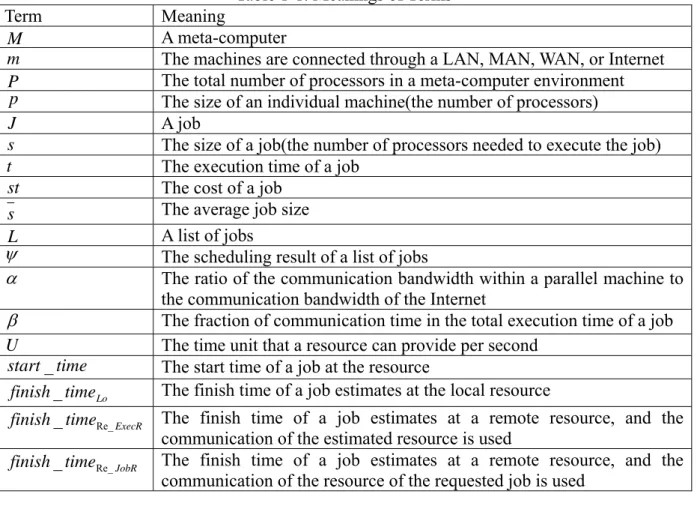
The symbols used in this study and their meanings are listed in Table 1-1：

Table 1-1. Meanings of Terms Term Meaning

M A meta-computer

m The machines are connected through a LAN, MAN, WAN, or Internet

P The total number of processors in a meta-computer environment p _{The size of an individual machine(the number of processors)}

J A job

s The size of a job(the number of processors needed to execute the job)

t The execution time of a job

st The cost of a job

s The average job size

L A list of jobs

ψ _{The scheduling result of a list of jobs}

α The ratio of the communication bandwidth within a parallel machine to the communication bandwidth of the Internet

β The fraction of communication time in the total execution time of a job U The time unit that a resource can provide per second

time

start _ The start time of a job at the resource Lo

time

finish _ The finish time of a job estimates at the local resource

ExecR

time

finish_ _{Re_} The finish time of a job estimates at a remote resource, and the

communication of the estimated resource is used JobR

time

finish_ _{Re_} The finish time of a job estimates at a remote resource, and the

communication of the resource of the requested job is used

We will begin explaining the following content of this study. Chapter 2 will discuss the related algorithms, which include four job scheduling algorithms, four processor allocation algorithms, and some cost models. Chapter 3 will further discuss the algorithms proposed in this study. The proposed algorithm is mainly focusing on the way to select computing resources and whether the job communication is necessary. By using this algorithm, we can obtain the computing resource that can finish the job the earliest. Chapter 4 will describe the experimental environment simulated in this study by using the GridSim simulation tool. Chapter 5 will explain the results and statistics obtained from the experiments. The last chapter will include related suggestions, directions for future development, and conclusions for the summarization of this study.

(15)

Chapter 2. Related Works

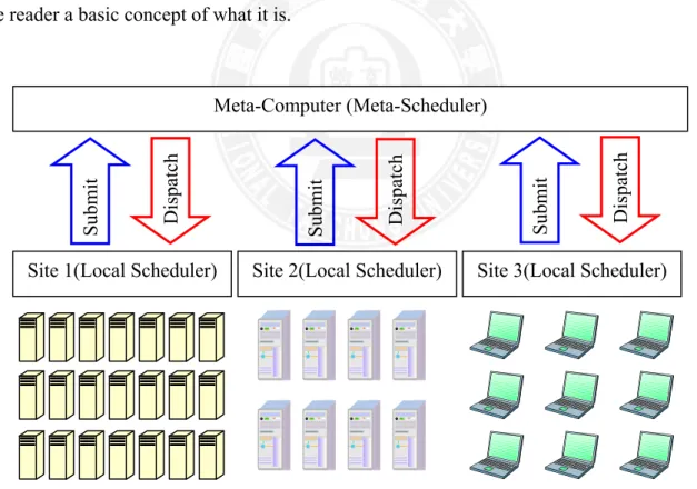
“Meta-computing” is a term two scholars, Smarr and Catlett proposed in 1992 [24]. The meta-computer is a network of computational resources that are linked together by internet and adequate intermediary software. They are just like multi-site computing, which distributes a job to different sites in parallel ways. By using this type of method, the user can distribute the job via a portal and not worry about how the job will be processed in the lower layers. Letting the user use the meta-computer in such a transparent way is just as easy as using a single computer, completely no fuss at all. This type of meta-computers that is formed via the internet can provide more computing power and services, which is something a current supercomputer cannot provide. Fig. 2-1 displays the architecture of the meta-computer to give the reader a basic concept of what it is.

Figure 2-1. Architecture of a Meta-computer

Adequate algorithms, such as job scheduling algorithms or processor allocation algorithms, must assist the process in order to effectively execute jobs in the Grid Computing

Site 1(Local Scheduler) Site 2(Local Scheduler) Site 3(Local Scheduler) Meta-Computer (Meta-Scheduler)

(16)

environment or a meta-computer. There are also some communication cost models that need to be considered. In this study, we will use combinational methods to discuss the ways to solve optimization problems of the job in the meta-computer environment. The following are divided into three parts, which are job scheduling algorithms, processor allocation algorithms, and cost models.

2.1 Job Scheduling Algorithms

In this section, we will briefly describe two types of job scheduling algorithms. The first is the First-Come, First-Served (FCFS) type; the other is the List Scheduling (LS) type.

2.1.1 First-Come, First-Served (FCFS)

The most simple, easily understood, and fair CPU scheduling algorithms within an operating system [22], [30] are the First-Come, First-Served scheduling type. Basically, FCFS policies have one queue, First-In, First-Out (FIFO) puts the CPU schedule into the queue. When the CPU is free, the CPU will start working on the first requested schedule in the queue. The requested schedules that are distributed and are executed will be removed from the queue. The data structure within computer sciences, also use FCFS algorithm. Every item will be placed in the queue by order; those that come in first will be processed first. It’s just like what people do when they enter a restaurant to eat or wait for a bus in line; the first in line will be served first and then the next person after that, and so on.

The brief introduction of FCFS algorithm used in this study will be in the following steps. The detailed content of FCFS algorithm is listed in Fig. 2-2.

(17)

1. Entering the first job.

2. Recycling the processors that have finished their job and assume they begin execution when the time begins.

3. Estimating of the job. When the amounts of processors in the system are not enough to execute the current job, the scheduling will go into a paused state. It will have to wait until other jobs are executed to release the processors. On the contrary, if the processors in the system are enough to execute the current job, then the processor allocation algorithm will be called to obtain the schedule of this job.

4. Removing the scheduled job from the job list. 5. Processing the next job in line.

Input: L=

(

J1,J2,K,Jn

)

, where n s s s₁≥ ₂ ≥L≥ for LJF; n t t t₁ ≥ ₂ ≥L≥ for LTF; n nt s t s t s₁₁≥ ₂ ₂ ≥L≥ for LCF. Output: ψ =

(

ψ1,ψ2,K,ψn

)

. Initially,

(

P₁',P₂',_K,P_m'

)

=

(

P₁,P₂,_K,P_m

)

; ' ' 2 ' 1 ' m P P P P = + +L+ .

At time τ =0, or whenever a job is completed at time τ , reclaim the processors used by the job just completed;

for (every J in L ) do i if ( ' P s_i > ) stop; else

call a processor allocation algorithm to get processor allocation

(

) (

)

(

)

(

Pj1,si,1 , Pj2,si,2 ,K, Pjm,si,m

)

;

generate the schedule of J as i ψi =

(

τ,

(

Pj1,si,1

) (

, Pj2,si,2

)

,K,

(

Pj_m,si,m

)

; i s P P' = '− ; Remove J from L ; i end if; end for; Figure 2-2. Algorithm FCFS

We use a simple example to explain FCFS algorithm. Suppose there are five jobs which need seven, ten, one, five, and three PEs to process. After FCFS algorithm scheduling, the

(18)

order of these five jobs become seven, ten, one, five, and three; the job receiving order is the job processing order.

When FCFS algorithm is used as the job scheduling algorithm, its advantages are: (1) fairness: the job the user requested will be processed in the order it was received. This is fair to the user, with no problems of competition. The job will always get the resource it needs; (2) it is easy to understand: the job received will not be processed into a new job processing order. The complexity will not be increased.

The disadvantages are (1) the job is time pressed: when the job processing is further back and has a deadline, then it faces the situation of not being finished at all; (2) using this type of algorithms to execute job scheduling, takes more time on average.

2.1.2 List Scheduling (LS)

The basic concept of LS algorithm is that all jobs have a certain type of priority. The jobs will be sorted according to their priority to produce a job list with new order. The following two steps will be repeatedly executed until all the jobs in the list have been scheduled [18], [25].

1. Selecting the job with the highest priority from the job list for scheduling. 2. Selecting one or some resources from the system to satisfy the job.

The job’s priority is preset before conducting scheduling processes. Therefore, the job order can only be decided when job scheduling begins. Well-known LS strategies include: the Earliest Starting Time first (EST), the Earliest Completion Time first (ECT), the Longest Processing Time first (LPT), and several others. They all decide the job processing order according to different priorities. In this study we choose to use Largest Job First (LJF). The biggest different compared to FCFS algorithm is that when there are not enough processors in the system to execute the current job, they will skip it and start on the next job in line for scheduling processes. Details of LS algorithm content are displayed in Fig. 2-3.

(19)

Input: L=

(

J₁,J₂,_K,J_n

)

, where n s s s₁≥ ₂ ≥_L≥ for LJF; n t t t₁ ≥ ₂ ≥_L≥ for LTF; n nt s t s t s₁₁≥ ₂ ₂ ≥_L≥ for LCF. Output: ψ =

(

ψ₁,ψ₂,_K,ψ_n

)

. Initially,

(

P,P, ,Pm

)

(

P1,P2, ,Pm

)

' ' 2 ' 1 K = K ; ' ' 2 ' 1 ' m P P P P = + +_L+ .

At time τ =0, or whenever a job is completed at time τ , reclaim the processors used by the job just completed;

for (every J in L ) do _i if ( ' P si > ) skip J ; i else

call a processor allocation algorithm to get processor allocation

(

) (

)

(

)

(

Pj1,si,1 , Pj2,si,2 ,K, Pjm,si,m

)

;

generate the schedule of J as i ψi =

(

τ,

(

Pj1,si,1

) (

, Pj2,si,2

)

,K,

(

Pj_m,si,m

)

; i s P P' = '− ; Remove J from L ; i end if; end for; Figure 2-3. Algorithm LS

We use a simple example to explain LS algorithm, while their priority setting is LJF. Suppose there are five jobs which need seven, ten, one, five, and three PEs to process. After the scheduling with LS algorithm, the processing order of these five jobs would become ten, seven, five, three, and one, with the largest job being first in line.

When LS algorithm is set as the job scheduling algorithm, the advantages are: (1) different priority settings can be used for different job list conditions in the system, thus changing the job execution order; (2) enhance the performance: processing jobs according to their priority means well resource management and use, this in turn increases the overall service quality. The disadvantages are: (1) unfair: jobs that queuing in the job list first will not be sure to be processed first; (2) if the system is in a dynamic scheduling state, jobs with lower priority may constantly be pushed back and robbed of resources because the system has received another new job request. Starvation states will result because of this.

(20)

2.2 Processor Allocation Algorithms

In this section, we introduce four types of processor allocation algorithms. The problem here would be how the processors should be allocated to the jobs, to obtain the optimal scheduling length. The algorithms here will be called after the process of the job scheduling algorithms, when there are enough processors for the job to use in the system. Therefore, we can suppose that every job in the job list will receive a scheduled outcome, such as

(

P_j₁,s_i_,₁

) (

, P_j₂,s_i_,₂

) (

,_K, P_jm,s_i_,_m

)

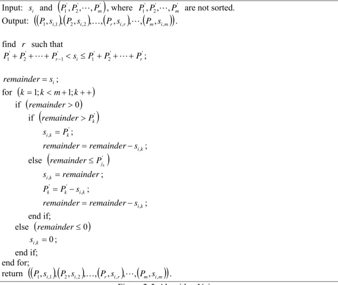
, when the jobs pass the processor allocation algorithms.

2.2.1 Naive

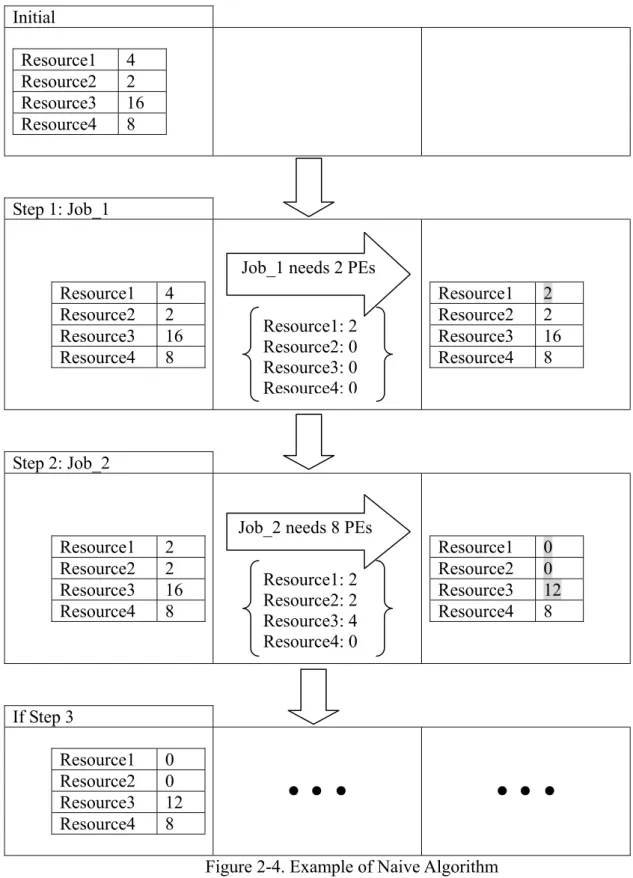
This is a simpler and naive algorithm. It thinks like this: resources in the system that can provide their PEs for the job’s demand means they will provide until the job’s demand is satisfied. For example, suppose there are four resources in the Grid environment, where Resource1 has four processors, Resource2 has two processors, Resource3 has sixteen processors, and Resource4 has eight processors; see the Initial in Fig. 2-4. These four resources have not gone through any assignment of order by priority. For instance, when a job requests for two processors, it will directly take away two processors from Resource1. Therefore, Resource1 is left with two processors; see Step one in Fig. 2-4. If the second job needs eight processors, it will take two processors from Resource1, two processors from Resource2, and four processors from Resource3. Then, Resource3 is left with twelve processors; see Step two of Fig. 2-4. After the dispatching of the two jobs, we only have twelve processors at Resource3 and eight processors at Resource4. See Fig. 2-5 for details of the Naive algorithm.

The advantage of this algorithm is: (1) the process method is simple and not complex. The disadvantage is: (1) for resources in the system, the optimal scheduling process is not conducted, therefore, wasting of resources or decreasing in the service quality may be occurred.

(21)

Initial Resource1 4 Resource2 2 Resource3 16 Resource4 8 Step 1: Job_1 Resource1 4 Resource2 2 Resource3 16 Resource4 8 Resource1 2 Resource2 2 Resource3 16 Resource4 8 Step 2: Job_2 Resource1 2 Resource2 2 Resource3 16 Resource4 8 Resource1 0 Resource2 0 Resource3 12 Resource4 8 If Step 3 Resource1 0 Resource2 0 Resource3 12 Resource4 8

…

Figure 2-4. Example of Naive Algorithm Job_1 needs 2 PEs

Resource1: 2 Resource2: 0 Resource3: 0 Resource4: 0

Job_2 needs 8 PEs Resource1: 2 Resource2: 2 Resource3: 4 Resource4: 0

(22)

Input: s and i

(

)

' ' 2 ' 1,P, ,Pm

P L , where P₁',P₂',L,Pm' are not sorted. Output:

(

P1,si,1

) (

, P2,si,2

) (

,K, Pr,si,r

) (

,L, Pm,si,m

)

.

find r such that

' ' 2 ' 1 ' 1 ' 2 ' 1 P Pr si P P Pr P + +_L+ ₋ < ≤ + +_L+ ; i s remainder= ; for

(

k =1;k <m+1;k++

)

if

(

remainder >0

)

if

(

'

)

k P remainder> ' ,k k i P s = ; remainder=remainder−s_i_,_k; else

(

'

)

k j P remainder≤ si,k =remainder; Pk' =Pk'−si,k; remainder=remainder−s_i_,_k; end if; else

(

remainder≤0

)

si_,k =0; end if; end for; return

(

P1,si,1

) (

, P2,si,2

) (

,K, Pr,si,r

) (

,L, Pm,si,m

)

.

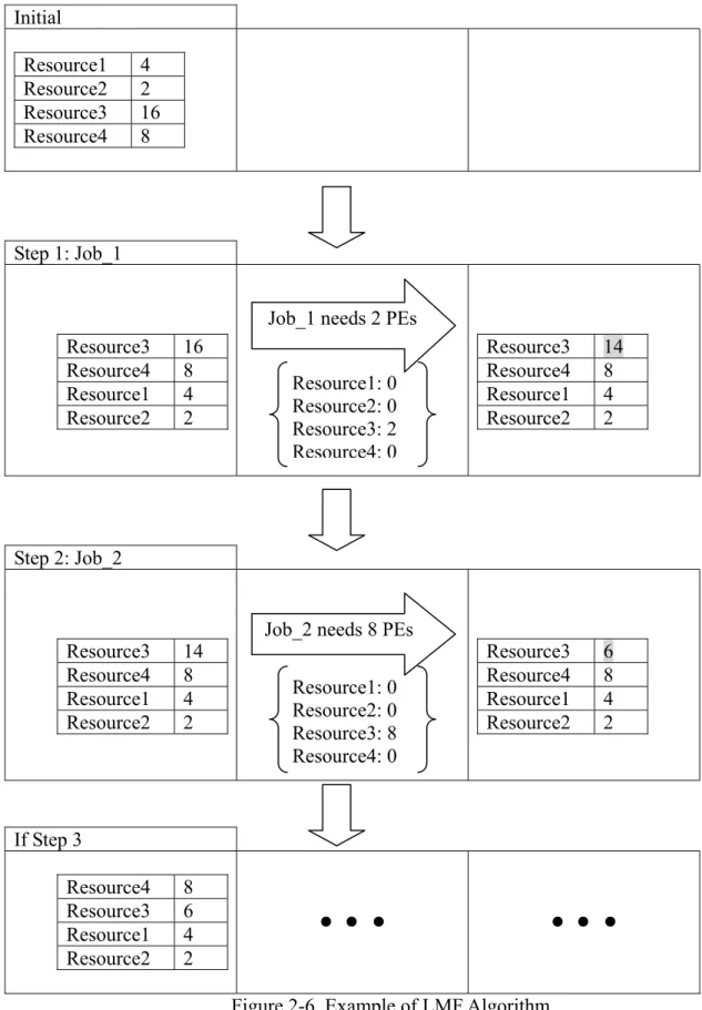
Figure 2-5. Algorithm Naive 2.2.2 Largest Machine First (LMF)

We can understand how this algorithm works just by reading Largest Machine First. It thinks like: resources in the Grid system will be sorted in an order according to their processor amount. This distributes according to the processor demand of the job. We continue using the example used in the Naive algorithm section. Suppose there are four resources in the Grid environment, where Resource1 has four processors, Resource2 has two processors, Resource3 has sixteen processors, and Resource4 has eight processors. The resources have to be sorted according to the processor amounts they have, from big to small. The distribution order would become Resource3→Resource4→Resource1→Resource2. When the first job requests two

(23)

processors, it will take two processors from Resource3; it is now left with fourteen processors, see Step one in Fig. 2-6. When the second job requests eight processors, the resources will be sorted again according to their processor amount. Now the resource order before the scheduling of the job would be Resource3→Resource4→Resource1→Resource2. Resource3 will allocate eight processors for the second job; Resource3 is now left with six processors, see Step two in Fig. 2-6. When there is a third job request, the resource order before the scheduling of the job would be Resource4→Resource3→Resource1→Resource2; see Step three in Fig. 2-6. Details of LMF algorithm may be seen in Fig. 2-7.

The advantage of this algorithm is: (1) when the job scheduling in the job list uses LJF algorithm, they will decrease the possibility of jobs being split into sub-jobs and the communication cost between sub-jobs. The disadvantage is: (1) when there are many jobs and the job scheduling in the job list uses Smallest Job First (SJF) algorithm, there may be lots of sub-jobs when scheduling proceeds to the larger jobs in the back, this in turn increases the communication cost of sub-jobs.

(24)

…

Figure 2-6. Example of LMF Algorithm Job_1 needs 2 PEs

(25)

Input: s and i

(

)

' ' 2 ' 1,P, ,Pm P L , where '₁ '₂ ' m j j j P P P ≥ ≥L≥ . Output:

(

P_j s_i

) (

P_j s_i

) (

P_j s_i_r

)

(

P_j s_i_m

)

m r , , 2 , 1 , , , , , , , , , , 2 1 K K .

find r such that

' ' ' ' ' ' 2 1 1 2 1 j jr i j j jr j P P s P P P P + +L+ ₋ < ≤ + +L+ ; i s remainder= ; for

(

k =1;k <m+1;k++

)

if

(

remainder >0

)

if

(

'

)

k P remainder> ' ,k k i P s = ; remainder=remainder−si,k; else

(

'

)

k j P remainder≤ s_i_,_k =remainder; P_k' =P_k'−s_i_,_k; remainder=remainder−si,k; end if; else

(

remainder≤0

)

(

P1,si,1

) (

, P2,si,2

) (

,K, Pr,si,r

) (

,L, Pm,si,m

)

. Figure 2-7. Algorithm LMF 2.2.3 Smallest Machine First (SMF)

The introduction of SMF algorithm can be compared with LMF algorithm; this is because the execution steps are the same as LMF algorithm. The only difference is their method of sorting the processors. Just by looking at the name, we can see that the allocating order of SMF algorithm is to set the resources with the least processors in the front. We still use the example used in Naive algorithm, the resources order here is sorted according their processor amount, which is Resource2→Resource1→Resource4→Resource3. The remaining steps are the same as LMF algorithm; it’s just that the resources are sorted according to their processor amount, from small to big. Fig. 2-8 for the execution process and Fig. 2-9 for the

(26)

details of SMF algorithm.

The advantage of this algorithm is: (1) when the job scheduling within the job list uses SMF algorithm, the possibility for jobs becoming sub-jobs decrease and the communication cost between sub-jobs decrease. The disadvantage is: (1) when job scheduling begins, the chance of a job being cut into sub-jobs and the amount of sub-jobs will increase, thus increasing the communication cost between them.

(27)

…

Figure 2-8. Example of SMF Algorithm Job_1 needs 2 PEs

(28)

Input: s and i

(

)

' ' 2 ' 1,P, ,Pm P L , where '₁ '₂ ' . m j j j P P P ≤ ≤L≤ Output:

(

P_j s_i

) (

P_j s_i

) (

P_j s_i_r

)

(

P_j s_i_m

)

m r , , 2 , 1 , , , , , , , , , , 2 1 K K .

find r such that

' ' ' ' ' ' 2 1 1 2 1 j jr i j j jr j P P s P P P P + +L+ ₋ < ≤ + +L+ ; i s remainder= ; for

(

k =1;k <m+1;k++

)

if

(

remainder >0

)

if

(

'

)

k P remainder> ' ,k k i P s = ; remainder=remainder−si,k; else

(

'

)

k j P remainder≤ s_i_,_k =remainder; P_k' =P_k'−s_i_,_k; remainder=remainder−si,k; end if; else

(

remainder≤0

)

(

P1,si,1

) (

, P2,si,2

) (

,K, Pr,si,r

) (

,L, Pm,si,m

)

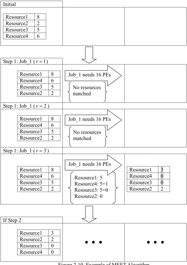
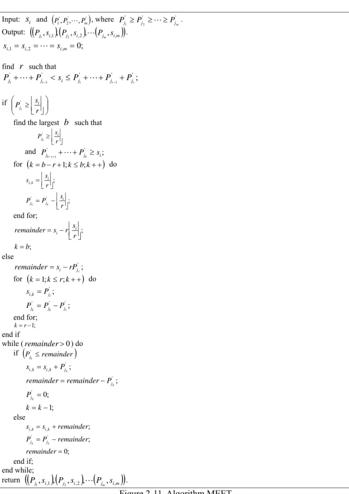
. Figure 2-9. Algorithm SMF 2.2.4 Minimum Effective Execution Time (MEET)

The goal of the MEET algorithm [17] proposed by Dr. Keqin Li is: when a job enters scheduling, try to minimize its effective execution time. The processing procedure of MEET algorithm are: every resource is sorted in order according to their amount of processors from big to small, find the resources that can provide enough processors for the job to execute, then evenly distribute the job to these different resources. MEET algorithm can avoid jobs splitting into too small sub-jobs and resulting in large communication times; it also conserves the resources that have more processors. See Fig. 2-11 for the details of MEET algorithm. We will then use a simple example to further explain this type of algorithm.

(29)

Suppose there are four resources in the Grid environment; Resource1 has eight processors, Resource2 has two processors, Resource3 has five processors, and Resource4 has six processors. A job that needs sixteen processors appears. The process for algorithm execution is listed below, see Fig. 2-10 for a diagrammatic illustration:

1. The resources are sorted according to their processor amount, from big to small. The order is Resource1→Resource4→Resource3→Resource2.

2. Whenr=1, splitting the job into one piece. Yet no resource can satisfy it.

3. Whenr=2, splitting the job into two pieces. Yet no two resources can provide the processors needed.

4. When r=3 , splitting the job into three pieces. Resource3, Resource4, and Resource1 can provide five processors. Since Resource2 does not enough processors, it cannot save Resource1 which has more processors. Therefore, Resource3, Resource4, and Resource1 can each provide five processors. A last processor is still needed, yet it cannot be provided by Resource3. Therefore, Resource4 will have to provide the last one processor. In the end, Resource3 has provided five processors, Resource4 has provided six processors, and Resource1 has provided five processors. 5. When the next job arrives, the resources will be sorted again, according to their

processor amount, which is Resource1→Resource2. Yet the job will have to pass the estimation of the job scheduling algorithm.

The advantages of this algorithm are: (1) it can avoid jobs being split too small and production of overlarge communication cost; (2) it can conserve the resources with more processors. The disadvantage is: (1) it only uses computation and no communication for computing, it may increase unnecessary communication cost.

(30)

Initial Resource1 8 Resource2 2 Resource3 5 Resource4 6 Step 1: Job_1 (r =1) Resource1 8 Resource4 6 Resource3 5 Resource2 2 Step 1: Job_1 (r =2) Resource1 8 Resource4 6 Resource3 5 Resource2 2 Step 1: Job_1 (r =3) Resource1 8 Resource4 6 Resource3 5 Resource2 2 Resource1 3 Resource4 0 Resource3 0 Resource2 2 If Step 2 Resource1 3 Resource2 2 Resource3 0 Resource4 0

…

Figure 2-10. Example of MEET Algorithm Job_1 needs 16 PEs

No resources matched

Job_1 needs 16 PEs No resources matched

Job_1 needs 16 PEs Resource1: 5 Resource4: 5+1 Resource3: 5+0 Resource2: 0

(31)

Input: s_i and

(

' '

)

2 ' 1,P, ,Pm P L , where Pj'1 ≥Pj'2 ≥L≥Pj'm. Output:

(

P_j s_i

) (

P_j s_i

) (

P_j s_i_m

)

m , 2 , 1 , , , , , , ₂ 1 L . ; 0 , 2 , 1 , = i = = im = i s s s _L

find r such that

; ' ' ' ' ' 1 1 1 1 jr i j jr jr j P s P P P P +_L+ ₋ < ≤ +_L+ ₋ + if _⎟⎟ ⎠ ⎞ ⎜⎜ ⎝ ⎛ ⎥⎦ ⎥ ⎢⎣ ⎢ ≥ r s P i jr '

find the largest b such that ⎥⎦ ⎥ ⎢⎣ ⎢ ≥ r s P i jb ' and ' ' ; 1 j i j P s P b r b−+ +L+ ≥ for

(

k=b−r+1;k≤b;k++

)

do ; ; ' ' , ⎥⎦ ⎥ ⎢⎣ ⎢ − = ⎥⎦ ⎥ ⎢⎣ ⎢ = r s P P r s s i j j i k i k k end for; ; ; b k r s r s remainder i i = ⎥⎦ ⎥ ⎢⎣ ⎢ − = else '; r j i rP s remainder = − for

(

k=1;k≤r;k++

)

do ; ; ' ' ' ' , r k k r j j j j k i P P P P s − = = end for; k= r−1; end if while (remainder>0) do if

(

Pj_k ≤remainder

)

' ; 1 ; 0 ; ; ' ' ' , , − = = − = + = k k P P remainder remainder P s s k k k j j j k i k i else ; 0 ; ; ' ' , , = − = + = remainder remainder P P remainder s s k k j j k i k i end if; end while; return

(

P_j s_i

) (

P_j s_i

) (

P_j s_i_m

)

m , 2 , 1 , , , , , , 2 1 L .

(32)

2.3 Cost Models

In the area of multi-site job scheduling, many researchers have discussed communication cost models. These models are all discussing the same problem; when a job is split into many sub-jobs and distributed to different machines for execution, and since additional communication time has appeared between the sub-jobs, how should we convert the computation time of a job into computation time and communication time? A job’s execution time is the time between the job starting time and the job finishing time. This period can be divided into the job computation time and the job communication time. The equation can be easily expressed asti =ti,comp +ti,comm . A job computation time is a job’s or sub-jobs’ computation time on a particular site. The job communication time can be divided into two types; one is the communication of the job or sub-jobs at different processors of the same site, the other is the communication of the job or sub-jobs at processors of different sites.

In reference [17], we are considering the communication time within the processor and outside of the processor. Therefore, we define the equation as equation (1):

α ⎟⎟ ⎠ ⎞ ⎜⎜ ⎝ ⎛ − + + = i k i comm i i k i comm i comp i k i s s t s s t t t*_, _, _, , _, 1 , (1)

This equation will divide the execution time into the job computation time, plus the communication time of the sub-jobs at certain resources, plus the communication time between the sub-jobs. This equation can be further simplified into:

(

)

_⎟⎟ ⎠ ⎞ ⎜ ⎜ ⎝ ⎛ − ⎟⎟ ⎠ ⎞ ⎜⎜ ⎝ ⎛ − + = 1 1 , α 1β * , i k i i k i s s t t (2) i comm i t t_, =

β is the fraction of the communication time of the job. From equation (2) we can see, when the value is large it means that the execution time is mostly spent on the communication. On the contrary, when the value is small, it means that the execution time is mostly spent on the computing. By using the equation above, we know the execution time of every sub-job and also know the job execution time after distribution, it can be expressed

as

(

*

)

, * 2 , * 1 , * _max _, _, _, t t t

(33)

time the job needs; this is because when the smallest sub-job needs more processors, it means the execution time the longest sub-job needs is shorter. The advantage of this research is: (1) after the job distribution is decided, we can quickly compute the execution length of the job. The disadvantages of this research are: (1) by processing the computing time and communication time separately, it may let the job be distributed to adequate resources, yet with inadequate communication bandwidth, causing the job execution time to increase; (2) it does not consider the internet heterogeneity of the sites; Sites vary in bandwidth. Yet this research set all bandwidth as equal and at the same speed.

( )

(

)

_⎟⎟ ⎠ ⎞ ⎜ ⎜ ⎝ ⎛ − ⎟⎟ ⎠ ⎞ ⎜⎜ ⎝ ⎛ ⎟ ⎠ ⎞ ⎜ ⎝ ⎛ − + = ≤ ≤ α 1β min 1 1 1 _, 1 * k i r k i i i s s t t i (3) In references [5], [39], the prerequisite is that all jobs in the multi-site scheduling environment must first be submitted to the Grid-Scheduler, and that all jobs can span across sites for executions. See Fig. 2-12 for the process of job submitting and distribution between the Grid-Scheduler and Site-Scheduler. All jobs distributed by the Grid-Scheduler will be distributed again according to the scheduling strategies within the Site by the Site-Scheduler. The following points can be used to explain this process:

1. All jobs produced in the site will pass through the job queue and submit to the Grid-Scheduler.

2. When the Grid-Scheduler has collected all jobs, it will start estimating the following points:

a. Is there one single Site that can provide enough PEs to finish the job on its own? b. If not then split the job into sub-jobs and distribute them to different sites on the

machine for execution. Yet they must all begin at the same time.

Since the jobs may be distributed to different sites for execution, we have to consider the overhead. The overhead is the cause of communication within the slow internet environments. A job’s execution time might have beent , yet after the influence of overhead it would i become *

i

t , which is the cause of internet communication factors. In this research, the cost

model will be expressed via equation (4):

(

p

)

t

t_i* = 1_i + (4) In this equation, p is considered a constant which is between 0% and 40%, with an

(34)

increment setting of 5%. The advantage of this research is: (1) the job’s execution time *

i

t

can be computed from the original computation time t and the overhead of the internet _i

communication time p . The disadvantage of this research is: (1) it has not considered the internet heterogeneity of the sites, although different sites will have the different bandwidth. In our study, we use the constant p in the equation to represent the overhead caused by the internet communication; which may cause the communication time to be less realistic.

Figure 2-12. Interaction between Site-Scheduler and Grid-Scheduler

In reference [12] the authors have proposed four types of cost model equations. If all the jobs in multi-site scheduling environments are divided into different sub-jobs and distributed to different machines for execution, then these four equations will be needed for computation of the job’s execution time. The equations mentioned in this research will be converted into symbols, which are listed in Table 2-1:

Grid-Scheduler

Site_1’s Scheduler

Job-Queue Job-Queue Job-Queue

(35)

Table 2-1. Transformation of Formulas The original equation After converting

(

)

f p + 1

(

)

ri i i t p t* = 1+

(

)

[

ri

]

i 1+p max

(

)

ik

)

i s r k i i t p t max 1 , 1 * ₌ ₊ ≤ ≤

(

1+p *

)

f t_i* = 1t_i

(

+ p

)

r_i

(

)

[

i

]

i 1 p *r max +

(

)

_i_k

)

r k i i t p s t i , 1 * ₌ _max ₁₊ ≤ ≤

f represents the amount of sub-jobs after the job is split into sub-jobs, this study uses

i

r to represent the amount of different sites that the job is distributed to for execution; r i represents the amount of computing resources every sub-job needs. This study uses s_i_,_k to

represent the amount of computing resources needed by every sub-job that is distributed to different sites; p represents the overhead value caused by the splitting of the job. A larger

p value means a longer average response time (ART). The four equations in this research,

all use the sub-job amount and the overhead value caused by the internet communication to evaluate the length of the job’s execution time. The advantage of this research is: (1) the job execution time can be quickly computed via the sub-job amount and the overhead value. The disadvantages of this research are: (1) processing the job computation time and the job communication time separately will cause good resources to be chosen with the inadequate communication bandwidth; (2) it has not considered the internet heterogeneity of the sites, although different sites will have the different bandwidth. In this research, the authors use the constant in the equation to represent the overhead caused by the internet communication; which may cause the communication time to be less realistic.

In reference [9], the authors used synchronous and asynchronous jobs to conduct experiments. The scheduler used in this research had to have the ability to predict the expected runtime via the machine and the processor it was using. This is because in a slow WAN internet environment, the amount of machines would affect the job processing time. Synchronous jobs mean that there exists a certain level of parallelism; the biggest difference between synchronous and asynchronous jobs would be the dependence issues related to the communication performance, and the expected runtime. Therefore, the authors proposed the following synchronous equation (5):

(36)

(

)

(

)

( )

⎥ ⎦ ⎤ ⎢ ⎣ ⎡ ⋅ ⎟⎟ ⎠ ⎞ ⎜⎜ ⎝ ⎛ − ⋅ + ⋅ ⎟⎟ ⎠ ⎞ ⎜⎜ ⎝ ⎛ ⋅ =

∑

− = − Sync BW BW r Comm P c S r Seq c c r Time WAN MPP M j j j r M Sync , , , : ₁ 1 1 φ 0 1 0 K with

{

}

{

}

(

)

(

, , | 0 1,1

)

min := Card c∈ c₀ c ₋₁ c> − Sync K M φ (5)

and asynchronous equation (6) for computing:

(

)

(

)

( )

⎥ ⎦ ⎤ ⎢ ⎣ ⎡ ⋅ ⎟⎟ ⎠ ⎞ ⎜⎜ ⎝ ⎛ − ⋅ + ⋅ ⎟⎟ ⎠ ⎞ ⎜⎜ ⎝ ⎛ ⋅ =

∑

− = − Async BW BW r Comm P c S r Seq c c r Time WAN MPP M j j j r M Async , , , : ₁ 1 1 φ 0 1 0 K with

(

)

∑

− = < ≤ − = ⋅ ⋅ − ⎟⎟ ⎠ ⎞ ⎜⎜ ⎝ ⎛ ⋅ = ₁ 0 0 1 0 max : _M j j j j j M j M j j j P c P c P c Async φ (6)

Equations (5), (6) in this research will be converted to symbols used in this study, such as equation (7):

(

)

(

i

)

r k k k i i i r P s S Seq t i 1 1 1 , * ₊ ₋ ⎟⎟ ⎠ ⎞ ⎜⎜ ⎝ ⎛ =

∑

= α β (7)

r represents a sub-job, we shall use i to replace it;c represents the amount of _i

processors needed by sub-jobs on a certain site, we use si,k to replace it; P represents the j amount of processors the site can obtain, we use P to replace it; k BWWAN is the bandwidth for the WAN communication, BWMPP is the communication bandwidth for the parallel computer, we use α to replace

WAN MPP

BW BW

; S_r_{( )}_n is the accelerating equation for n processors;

( )

r

Seq represents the runtime of the job at a single processor; Comm

( )

r represents the communication part of the entire job execution time, we use β to replace it. The equation proposed in this research is similar to equation (3) in reference [17]; they all use the execution time of sub-jobs to compute the job execution time. The advantage of this research is: (1) the job execution time can be obtained by computing the sub-job execution time. The

(37)

disadvantages of this research are: (1) by processing the computing time and the communication time separately, it may let the job be distributed to adequate resources, yet with the inadequate communication bandwidth, causing the job execution time to increase; (2) it has not considered the internet heterogeneity of the sites, although different sites will have the different bandwidth and the unstable communication time in the internet communication.

In order to make the computation of the job execution time more realistic, when we are computing the job execution time, we should also consider the job computation time and the job communication time. This will avoid letting the job have fine resources for execution, yet go through the unnecessary communication time; the job communication can also be estimated necessary or not by considerations of the internet communication; if not, the communication of the job can be saved.

(38)

Chapter 3. Proposed Algorithm

In chapter 3.1 we will define the problems of the experimental environments in this study; 3.2 displays the algorithm proposed in this study; 3.3 gives a few simple examples to explain the algorithm proposed in 3.2 .

3.1 Problem Definition

First let’s hypothesize the basic environment architecture in this experiment. In this study, the meta-computer environments within the experiments, we have hypothesized that the computing grid is made up of several independent resources, and that several nodes (A node is equivalent to a machine) are within every resource, while every node has a different amount of processors, storage, memories, local workloads, etc. In every resource, different nodes can be linked together via the fast interconnection network. In this study, different amounts of nodes within different resources will be used in different meta-computer environments (four different types of meta-computer environments are used in this experiment). Other than that, the architecture setting for every node will be set as heterogeneous, causing the processor amount and the processor MIPS rating to differ; the heterogeneity will happen at random. See Fig. 2-1 or Fig. 3-1 for the architecture of the meta-computer. In the experimental environment architecture of this study, every resource will have its own site scheduler to construct a meta-computer on every resource to form this environment. Within the meta-computer is a Grid-Scheduler (or a Meta-Scheduler) that is responsible for receiving all job requests of the resource to conduct computing and coordination of job distribution. When the computing of the Grid-Scheduler is finished, the job will be dispatched to the adequate resource for execution. The dispatched job will be received by the site scheduler and processed according the policy within the resource. Therefore, in the experimental environment of this study, the Grid-Scheduler acts as a centralized scheduler, computing and coordinating the distribution of the job.

(39)

Figure 3-1. Architecture of a Meta-computer

Several types of resources and jobs exist in real environments, and before the job finds the suitable resource, it has to conduct preselection on the resources within the grid system. This action will filter out the suitable resources for use. Therefore, since there are different types of resources and job requests, it will restrict the amount of resources a job can find to use. In this study, we neglected this preselection process between the resource and the job, and focused on the scheduling results. Therefore, we supposed that all resources are of the same types and that all jobs could execute on all of the resources; we also set the machine processor as a Space-Shared model. Processors of this model will focus on finishing one job after the distribution jobs, instead of working on two different jobs at the same time. Next, we will define the problems of the experimental environments of this study.

The grid computing within the meta-computer environment will express the meta-computer asM =

(

U₁,U₂,_K,U_m

)

, U is the job time unit provided by every resource _j

every second (for example: one 10 MIPS processor can provide 10 job time units every second), 1≤ j≤m(m is the number of resources within a meta-computer), and a list of jobs will be expressed as L=

(

J1,J2,K,Jn

)

. Every job within the list will be expressed asJ , i

n i≤ ≤

1 (n is the number of job requests within the job list that needs to be processed). s _i

is the amount of processors needed for the execution of this job; t is the amount of MIPS i

Site_1 Site_2 Site_3

(40)

needed to process the job on a single processor (this study replaced the MIPS demand with the job time unit). In the GridSim simulation tool, the standard format “Gridlet (id, length, file_size, output_size)” displays the related data of the job. The length equalst ; numPE is _i

used to express the amount of processors needed to execute the job, which iss . As for every i

i

J in the job list L , the goal of this study would be to find out the resource that can obtain

the “earliest finish time” of the job, thus obtaining the shortest computation time for the job list to acquire a “earliest finish time” for the job list. Therefore, we need to know (1) the total job time units and the communication bandwidth needed for every resource; (2) the amount of processors and job time units needed to execute the job; and (3) the job starting time and the job finishing time at every resource. By using the data above to compute the earliest finish time for every job at every resource, the jobs can be distributed to resources that can finish executing the earliest.

3.2 Proposed Algorithm

The content of the proposed algorithm in this study is listed in Fig. 3-2. The execution process contains the following steps. We will explain these concepts respectively according to their analyzing procedures:

1. First of all, the input statistics ares , which express the jobs for processing; they are i expressed via the standard format of GridSim “Gridlet (id, length, file_size, output_size)”. In this study, the length is converted into “job time units”;

(

' '

)

2 '

1,P, ,Pm

P _K expresses the “total computing power (which are converted to total

job time units the resource have)” of the resource in the Grid system.

2. The throughput results we hope to obtain will be expressed as

(

)

f s j j j i P P P s , , , . The i of s is the job’s ID (the ID of the Gridlet), andi s is the ith job in the job list; the j i of P is the Resource_ID of the obtained earliest_finish_time, andj P is the j resource the job executed;

s

j

P is the job’s start_time;

f

j

異質性網格計算環境中之工作排程與處理器配置

國立台中教育大學數位內容科技學系碩士論文

指導教授：賴冠州 博士

異質性網格計算環境中之工作排程與處

理器配置

Job Scheduling and Processor Allocation

for Heterogeneous Grid Computing

Environments

研 究 生：楊大猷 撰

中 華 民 國 九 十 六 年 七 月

摘要

Abstract

Table of Contents

List of Tables

List of Figures

Chapter 1. Introduction

1.1 Motivation

1.2 Problems

1.3 Purposes

1.4 Restrictions

Chapter 2. Related Works

2.1 Job Scheduling Algorithms

(

)

(

)

(

)

(

)

(

) (

)

(

)

(

)

(

(

) (

)

(

)

)

(

)

(

)

(

)

(

)

(

) (

)

(

)

(

)

(

(

) (

)

(

)

)

2.2 Processor Allocation Algorithms

(

(

) (

) (

)

)

…

…

(

)

(

(

) (

指導教授：賴冠州博士

研究生：楊大猷撰

中華民國九十六年七月