Iterative Repair Approach to Job Shop Scheduling in a Dynamic Environment
12
0
0
全文
(2) 2. Sur vey 2.1 J ob-shop Scheduling as Optimization Since the performance measure of a scheduling problem can be quantified as an objective (cost) function, the scheduling problem becomes to minimize/maximize the objective function while satisfying specified constraints. In other words, the problem can be modeled as a constrained optimization problem. In this subsection, we will introduce how to model the job-shop scheduling problem as a constrained optimization problem. For convenience, the notations to be used in this paper are shown as follows, where operation j of job i is referred to as operation (i, j). N: Number of jobs. M: Number of machines. sij: Start time of operation (i, j). Ri: Ready time of job i. cij: Completion time of operation (i, j). Ci: Completion time of job i. pij : Processing time of operation (i, j). P i: Total processing time of job i. mij: The Machine processing operation (i, j). di,j: Due date of operation (i, j). Di: Due date of job i. Ti: Tardiness of job i. ui: Tardiness weight for job i. The following assumptions are made for the problem: (1) all the jobs are available at time zero, (2) operation processing is assumed to be nonpreemptive, (3) processing time of the jobs on the machines are known beforehand. A static and deterministic scheduling problem can now be formulated as a constrained optimization problem:. P : min J ,. (1). The objective function J , minimum weighted tardiness, is defined as follows: N. J = ∑ viTi. (2). i =1. where the weight vi times the job tardiness Ti represents the job tardiness penalty. The minimization of objective function J is subject to four types of constraints: operation precedence constraints, machine capacity constraints, processing time requirements and ready time requirements. Each constraint is described below.. 1) Operation precedence constraints: The operation precedence constraints require the completion time of an operation cij to be less than or equal to the start time of its succeeding operation si,j+ 1 , i.e.,. cij. si,j+ 1 (i=1,2,..,N; j=1,2,… ,M-1) (3). 2) Machine capacity constraints: The machine capacity constraint requires that there is no overlapped processing time between two operations sharing the same machine. if mij = mi',j' , then sij - si',j' p i',j' or si',j'- sij pij (i,i’= 1...N; i i’; j,j’= 1...M). (4). 3) Processing time requirements: The processing time requirement for operation (i, j) means that the elapsed time between the start time sij and the completion time cij should be pij, i.e.,. cij - sij = pij (i= 1, 2, ., N; j= 1, 2, .., M) (5) 4) Ready time requirements: The ready time requirement states that the start time of the first operation of each job is greater than or equal to zero, i.e.,. si1 0 (I=1,2,… ,N). (6). Corresponding to the four types of constraints are four types (Type I - IV) of conflicts that may arise during the scheduling process. For instance, Type I conflict corresponds to the violation of operation precedence constraint. Each conflict is associated with either one operation (Type III and IV) or two operations (Type I - II).. 2.2 Local-search-based Algor ithms Since the job-shop scheduling problem is NP-hard, it is unlikely that a practical approach to this scheduling problem can yield an optimal solution. Therefore, one could even use an exact method to find an optimal solution for small problem instances. But for lager problem instances it is more appropriate to use heuristics or approximation algorithms, such as local-search-based algorithms, to find a good solution that is not necessarily the optimum one. Local-search-based algorithms include local search[3], simulated annealing[6], or tabu search[4]. These search techniques are very efficient in solving combinatorial optimization problems. 1) Local Search (local improvement): Local search [3,7] is one of the few successful.
(3) techniques for combinatorial optimization problems. Assume that vector x represents the set of values assigned to the decision variables and a neighborhood N(x) is defined for x. Now given a solution point xk and an objective function f(x) to be minimized (or maximized), a solution point xk+ 1 is searched from the neighborhood N(xk) of xk such that f(xk+ 1) < f(xk) ( or f(xk+ 1) > f(xk)). The drawback of local search is that it has a tendency of getting stuck at a local optimum (or a cycle). 2) Simulated Annealing: Simulated annealing can be regarded as a variation of local search. The main difference is that, in simulated annealing, each solution point in the neighborhood of the current search point is selected with a certain probability for the next search step. Such a difference makes it possible to keep the algorithm from getting stuck at a local optimum by permitting uphill moves. Its drawbacks include the following: its performance is heavily influenced by the initial temperature and the decrement ratio of the temperature, context-sensitive search behavior, and it could be potentially time consuming when applied to complex problem instances. 3) Tabu Search: Tabu search was introduced by Glover [2]. The underlying idea is to forbid some search directions (moves) at a present iteration in order to avoid cycling and escape from a local optimal point. This strategy can make use of any local improvement technique.. 2.3 Previous Approaches to J ob Shop Scheduling In the past, dispatching rules, job-ordering approach and Lagrangian relaxation methods are known to be practical approaches for solving job-shop scheduling problems. In the following, they are briefly introduced. 1) Dispatching Rules: Dispatching rules are a distributed sequencing strategy, by which a priority is assigned to each job waiting for service on a machine: whenever a machine is free, the one with highest priority is selected. Here the following rules will be considered: their purposes are to provide a comparison for the proposed scheduler. a) Shortest Processing Time (SPT) rule b) Longest Processing Time (LPT) rule c) Earliest Due Date (EDD) rule d) Operation Due Date (ODD) rule e) Modified Operation Due date (MOD) rule f) Operation Priority Index (OPI) rule 2) Job-Ordering Approach: Several algorithms based on iterative improvement approach have been developed to find a. reasonably good schedule [4, 6]. In their approaches, the disjunctive graph representation was introduced as a useful representation of operation precedence in the context of minimizing the makespan in a job shop. The search techniques can be local search, simulated annealing, or tabu search. Although the job-ordering-based approaches had been successfully applied to job-shop scheduling problems, they can not be applied to those problems with non-regular performance measure. 3) Lagrangian Relaxation (LR): Recently, scheduling methodologies based on LR have proven to be computationally efficient and have provided near-optimal solutions to job-shop scheduling problems [1]. By use of LR techniques, the scheduling problem is decomposed into operation-level subproblems for the selection of operation beginning times and machine types, with given multipliers and penalty coefficients. The solution forms the basis of a list-scheduling algorithm that generates a feasible schedule. The comparison between LR techniques and our approach will be given in Section 6.. 3. Repair -based Appr oach Repair-based approach starts with a complete but possibly infeasible schedule and then searches through the space of possible repairs. The search can be guided by a repair heuristic, such as min-conflicts heuristic [5] that attempts to minimize the number of constraint violations after each step. A variety of different search strategies can be embedded in the repair-based system, such as local search, simulated annealing, and tabu search.. 3.1 Problem For mulation Mathematically, the scheduling problem can be formulated as a constrained optimization problem (see Section 2). We can transform the constrained optimization problem to an unconstrained optimization problem via Lagrange multiplier [9]. Assume that X is a solution point (or a schedule) and can be expressed as. X = xij, 1 i N and 1 j M. (7). where N is the number of trains and M is the number of stations. Each xij is associated with operation (i, j) and a triplet [sij, cij, mij] corresponding to start time, completion time, and machine. The new objective (cost) function is defined as. C(X) = J (X) + ëQ(X) + ãJ AUX(X). (8).
(4) where J (X) represents the original objective function, which is our measure for schedule quality, described in Section 2.1, J AUX(X) represents the auxiliary objective function used to facilitate the scheduling process, ã is the coefficient of auxiliary objective function, Q(X) is the cost due to the conflicts in schedule X, and ë is the Lagrange multiplier used to relax the constraint violations. We usually refer the objective function C(X) to the cost function of the problem. For simplicity, we call C(X), J (X) and Q(X) the total cost, the performance cost and the conflict cost of the schedule, respectively. The coefficient ã in EQ. (8) is selected based on experiences, which is less than 1 because J AUX(X) is less important compared to J (X); the Lagrange multiplier ë is chosen to satisfy ë>>1 since a conflict-free schedule is our ultimate goal. Q(X) is defined as ∑K ( X ) qk , where qk is a positive k =1. integer representing the time interval of the kth conflict and K(X) is the number of conflicts in schedule X .. 3.2 Proposed Algor ithm Similar to [9], the proposed system consists of four basic components: Initial Scheduler, Repair Scheduler, Local Scheduler and Conflict Management. First, an initial schedule is established according to the predictive schedule and the affect of real environment regardless of constraint violations. The Repair Scheduler then determines the sequence of conflicts to be repaired according to Earliest-Conflict-First heuristic after the Conflict Management finds all conflicts in the initial schedule. Then the Local Scheduler resolves the conflict given by Repair Scheduler while minimizing the objective function. 1) Repair Methods: Recall that each conflict is associated with either one operation (Type III and IV) or two operations (Type I and II). The system will try to shift the violated operation left or right on the time axis as long as the conflict is released, rather than exploring many possible alternatives. There are three repair methods that can repair a conflict: a) Swap(SP): Swap the start time of the two violated operations. This repair method is suitable for capacity constraint violations. As we swap the two operations contributing a capacity constraint violation, the violation may disappear or be alleviated. b) Left-Shift(LS): Left-shift the violated operation on the time axis such that the violated constraint is satisfied. This repair method can be applied to all types of conflicts except the ready time conflict. c) Right-Shift(RS): Right-shift the violated operation on the time axis such that the violated. constraint is satisfied. This repair method can be applied to all types of conflicts. To resolve a conflict, one of the repair methods will be selected in an attempt to reduce the cost function as much as possible. If the selected repair method is LS or RS, then one of the operations contributing the conflict will be moved. The heuristic used to select the operation to be moved considers the suitability of the operation to the repair method applied to the conflict. Furthermore, to facilitate the selection of repair methods for a conflict, we specify the priority of each repair method, such that the repair method with higher priority will be tried first. The priority is given in the following sequence: SP > LS > RS. The priority of SP is higher than that of LS(RS) because the SP can change the sequence of the two conflicting operations, whereas the LS(RS) can not. Although the RS has lower priority, it plays an important role in our repair-based scheduling system. Since the RS would not create a conflict which is on the left of the conflict-free boundary on the time axis, it can facilitate the expansion of the conflict-free area. Notice that the proposed repair methods will not affect the operation processing times. Thus, Type III conflict would not arise during the scheduling process. 2) Iterative Repair : Initially, the initial schedule is established according to the dynamic environment. Since the initial schedule is not conflict-free, we iteratively search a repair that resolves the conflict given by the Earliest-Conflict-First heuristic while minimizing the cost function. To select an appropriate repair method for a conflict, local search techniques can be used. During the kth iteration, we iteratively search a repair that resolves the given conflict and minimizes the cost function at the same time. The iterative repair algorithm based on local search is shown in Figure 1, in which the following notations are used: SC : The set of conflicts corresponding to current local schedule SR : The set of repair methods co : The cost of the original local schedule. cn : The cost of the new generated local schedule count : the number of iterations Since local search techniques suffer from the cycling problem, i.e., a cycle may exist among a sequence of repair operations, a cycle detection and prevention scheme is required. In the following subsection, we will introduce how to detect and prevent cycles..
(5) 3.3 Cycle Detection and Prevention The local search algorithm has a tendency of getting stuck at a local optimum or a cycle. For example, there is a capacity constraint violation between two operations at some machine, and the earlier operation has been shifted earlier to repair the conflict. But the shift results in another new capacity constraint violation. To repair the new conflict, the operation has to be shifted later and hence the original conflict comes back. Therefore, a cycle occurs between the two repair operations. A cycle occurs when the schedule is unchanged after a sequence of repair operations. Since different values of cost function C(X) always correspond to different schedules, we can easily verify that two schedules are not identical if they have different C(X) values. On the other hand, two schedules with the same C(X) values may not be identical. From the above observations, we incorporate a forbidden list into the standard local search algorithm. We use the C(X) value of each intermediate schedule as the element of the forbidden list. We can conjecture that a repair may result in a cycle when the C(X) value of the schedule resulting from this repair hit the forbidden list (i.e., the value is equal to one of those stored in the forbidden list). If the C(X) value of the current schedule is not found in the forbidden list, we can quickly ascertain that a cycle does not exist; otherwise a cycle may exist and a further investigation is required. We employ another list called action list to memorize the information about each recent repair. From the action list, we can realize the transition of the intermediate schedule and find out whether the intermediate schedules having the same C(X) values are actually identical. Once there is a hit on the forbidden list during the repair process, we have to examine the action list that the repairs between the two intermediate schedules having the same C(X) values in order to make sure that whether a cycle exists or not. When a repair method results in a cycle, we try next priority repair method unless the repair method is the last repair method. In the following we define the variables and the repair operations more precisely. Definition 1: (Variables) There are three variables associated with an operation, i.e. s( i, j), c(i, j) and m(i, j), which represent the start time, the completion time and the machine assignment of the jth operation of job i, respectively, assuming that operation j of job i is referred to as operation (i, j). The total number of variables is equal to 3NM, where N is the number of jobs and M is the number of machines. Definition 2: (Repair operations, Characteristic pattern, Numeric parameter ). Each repair operation is represented by F(i, j, Rk , Ä ). It is associated with four parameters: i (the job index), j (the operation index), Rk (the type of repair operation) and Ä (the amount to be changed), A repair operation modifies the values of a set of variables and the variables depend on the job index and the operation index (see Definition 1). The combination of the first three parameters is called the characteristic pattern of the repair operation, which identifies which variables are to be modified by the repair operation, and the last parameter is called the numeric parameter which specifies the degree of the value(s) of the variable(s) to be changed. Actually, each element of the action list records the four parameters of the associated repair. In the following, we introduce a primitive repair operation that composes the proposed three repair methods. Definition 3: (Primitive operation: shift operation) The shift operation F(i, j, SHIFT, Ä ) shifts the operation (i, j) on the Gantt chart. The variables to be modified are shown as follows:. s(i, j):= s(i, j) +Ä and c(i, j):= c(i, j) +Ä. (9). Definition 4: (Cycle) If the schedule is unchanged after a sequence of repairs, then we say that there is a cycle among the sequence of repairs. From the above definitions, we can derive the following properties and theorems to support our cycle detection method. Property 1: Using the primitive repair operations defined in Definition 3, different characteristic patterns refer to different variable(s) and all possible characteristic patterns cover all variables. From Gantt chart's point of view, the schedule can be seen as a collection of rectangles, each of which represents an operation. Each of the rectangles is associated with two variables, i.e., the start time and the completion time of the operation. The difference between the two times corresponds to the processing time of the operation, which depends on the performed machine of the operation. Definition 3 implies that each rectangle is characterized by a particular characteristic pattern and is controlled by the shift operations with the same characteristic patterns. The shift operation F(i, j, SHIFT, Ä ) controls the position of the rectangle associated with operation (i, j) on the Gantt chart. Thus, the primitive repair operation, shift operation control all of the variables. In conclusion, different characteristic patterns refer to different variable(s) and all possible characteristic patterns cover all variables. Property 2: The schedule is unchanged, if.
(6) and only if the sum of the numeric parameters of the repair operations with the same characteristic pattern is zero. If the schedule is unchanged then the value of each variable must be unchanged. In other words, the operation applied to each variable has no effect. Since each variable is associated with a particular characteristic pattern, it is uniquely controlled by the repair operations with the same characteristic patterns. Thus, if the value of a variable remains unchanged then the combination of all changes to the variable must be zero, i.e., the sum of the numeric parameters of the repair operations with the characteristic pattern associated with the variable is zero. From the above properties, we can devise an algorithm used for cycle detection (see Figure 2). Let ALIST denotes the part of the action list which is required to be examined. The ALIST records the parameters (see Definition 2) of the sequence of repairs between the two schedules having the same cost value. Since the above properties only hold for primitive repair operations, the aforementioned three repair methods have to be stored in the action list in their primitive forms. The algorithm returns TRUE if a cycle is detected and returns FALSE otherwise.. 3.4 Semi-active Timetabling Since regular performance measures [8] are non-decreasing in the job completion times, superfluous idle time among operations will deteriorate the schedule quality. Superfluous idle time exists in a schedule if some operation can be started earlier in time without altering the operation sequences on any machine. Given an operation sequence for each machine, there is only one schedule in which no superfluous idle time exists. The set of all schedules in which no superfluous idle time exists is called the set of semi-active schedules. This set dominates the set of all schedules, which means that it is sufficient to consider only semi-active schedules to optimize any regular measure of performance. Therefore, we have to remove the superfluous idle time in the schedule generated by the repair-based approach. This work can be done by semi-active timetabling [8]. Timetabling is the process whereby we derive a schedule from a sequence. In semi-active timetabling the processing of each operation is started as soon as it can be.. 4. STATIC Schedule gener ation 4.1 Initial Schedule Gener ation Since repair-based algorithm is a kind of local search algorithm, we must generate an appropriate initial schedule so that the resulting. final schedule will be acceptable. Through the combination of local search techniques and an appropriate starting point, the system can quickly find a good feasible solution. For this purpose, we generate an initial schedule X according to the following heuristics: 1) The schedule has the minimum value of J (X). 2) The schedule satisfies all types of constraints except the capacity constraints. This is because other types of constraints need not to consider the interaction among jobs, and can be satisfied directly through dispatching. 3) The processing times of operations must be appropriately distributed on the time axis such that the number of capacity constraint violations in the initial schedule can be reduced, and the burden of the repair-based system can be alleviated because the number of conflicts to be resolved is reduced. Therefore, we can divide the scheduling process into two parts: the initial scheduling process and the iterative repairing process. In the initial scheduling process, the capacity constraints are relaxed and the initial schedule is generated optimally with respect to J (X); in the repairing process, the system coordinates the operations to find a good conflict-free schedule. In the following, we propose four methods to generate an initial schedule: 1) Dispatch by CON Rule (DCON): The operation due-dates dij generated by CON (constant flow allowance) rule are assigned to the corresponding completion times of operations, cij. 2) Dispatch by TWK Rule (DTWK): The operation due-dates dij generated by TWK (proportional to total work) rule are assigned to the corresponding completion times of operations, cij. 3) Dispatch by Constant Slack Time Rule (DCST): The slack time of an job i, Si , is defined as Si = Di - Ri - P i , where Di , Ri , and P i represent the due-date, ready time and total processing time of the job, respectively. The due-date of a job is assigned to the completion time of the last operation, and a constant idle time (Si / M) is inserted between successive operations and between the first operation and ready time. 4) Dispatch by Modified Constant Slack Time Rule (DMCST): This rule is similar to DCST except that the constant idle time is (Si / (M+1)). Besides, the constant idle time is inserted between the last operation and the due-date of the job. Note that the completion(start) time of an operation is determined according to the.
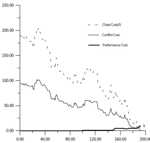
(7) processing time requirement once the start(completion) time of the operation is determined. Method (1)-(2) are motivated by the operation due-date rule CON and TWK. Since ODD dispatching rule with due-date rule CON/TWK performs quite well, it hints that the sequence given by the dispatching rule can be treated as a good initial sequence. Therefore, it is reasonable to expect that the initial schedule based on CON/TWK rule would be a good initial schedule. Method (3)-(4) are developed straightforward, which intend to distribute the operations uniformly on the time axis.. 4.2 Test Results In the following experiments, the coefficients in the cost function are assigned according to the comments in Section 3.1 and testing experiences. As such, the Lagrange multiplier ë was set to 10, and the coefficient of the auxiliary objective function, ã, was set to 0.3. The operation due-dates used in auxiliary objective function was set according to CST(constant slack time) rule as depicted in Section 4.1, since we found that the CST rule performs better than all of the other rules in our system. In this paper, all experiments were run on a PC with Cyrix 6X86-P120(100MHz). The computer program was written in C language. Each experiment ran until the resulting schedule was conflict-free. We randomly generate three 10-job 10-machine problems according to the following problem factors: • Processing Time: The processing time of each operation is uniformly distributed between 1 and 10; • Due Dates: The due date of each job is set to the total processing time of the job times a DSF (due date set factor), where the DSF is uniformly distributed between 1 and 3. Table I-III show the numerical results for the three problems with weighted tardiness objective. For simplicity, the weight of job tardiness in EQ. (2), vi , is set to 1. Table I reports the results of these problems solved by the priority dispatching rules described in Section 2.4. We can find that the ODD rule generates the best average cost, 41.3, for the three problems. Table II reports the results of the three problems solved by the repair-based approach combined with semi-active timetabling. The forbidden/action list size is set to 15. Among the different methods of initial schedule generation, we find that the DTWK generates the best average cost, 25.3, which is also better than that generated by ODD dispatching rule. The average CPU time is 0.51 seconds. In Figure 3, we graph the cost as a function of iteration for the problem solved by the proposed. algorithm. The three curves in the figure represent the conflict cost, the performance cost and the total cost of the schedule (see EQ. (8)), respectively. Each iteration corresponds to a repairing cycle. Although the performance cost is increasing, the total cost is decreasing. The conflict cost achieves zero, i.e., conflict-free, after 192 iterations. The performance cost obtained is 9, and is reduced to 7 after semi-active timetabling. To show the effectiveness of the incorporation of auxiliary objective function J AUX to the cost function C in EQ. (8), we also test the problems solved by the same approach without considering the auxiliary objective function. This is equivalent to setting ã in EQ. (8) to 0. The results are shown in Table III. We can find that, for most cases, the performance cost is higher than the cost with the auxiliary objective function. The experimental results show that: (1) The repair-based approach compares advantageously with heuristic dispatching rules in terms of schedule quality. Although different initial schedule generation methods may result in different schedule quality, we find that DTWK is the most appropriate initial schedule generation method for due-date-based performance measures. The repair-based approach with DTWK performs better than all of the priority dispatching rules in terms of schedule quality. This is due to the fact that the priority dispatching rules are too myopic, whereas the initial schedule generation method DTWK provides sufficient global information of the search space and hence guide the local search to yield better quality schedules. (2) Through the incorporation of the local search technique and the cycle prevention scheme, the repair-based approach can produce a conflict-free schedule. (3) The Earliest-Conflict-First heuristic makes the scheduling system more efficient and effective. (4) For most cases, the employment of the auxiliary objective function enables a lower performance cost J to be found.. 5. DYNAMIC RESCHEDULING In real world applications, algorithms searching for optimal schedules quickly break down due to the dynamic and stochastic nature of the factory environment. Unexpected events such as machine breakdown, operation tardiness, reworking, new orders, and so on, will force changes to previously planned activities. According to the characteristics of unexpected events, we divide the unexpected events into two categories: 1)disturbance: the events which will not affect the number of jobs, such as machine.
(8) breakdown, operation tardiness, reworking. 2) job insertion/deletion [10]: the events which affect the number of jobs, such as new orders. In order to react to unexpected events, we use some heuristics to modify the predictive schedule and feed the modified schedule into the repair-based system. Then the system will automatically repair the conflicts and result in a new predictive schedule. In the following subsections, we will introduce how to react to these unexpected events.. 5.1 Distur bance To react to disturbance, we can modify the original schedule according to disturbance and then apply repair-based approach to resolve the conflicts in the schedule. Let's look at the following example. As shown in Figure 4, there is a schedule for a randomly generated 5-job 5-machine problem. Assume that Machine_2 breaks down during time interval (0, 20). To react to the event, we shift the operations performed on Machine_2 right such that no operation needs to be performed on Machine_2 during the time interval. In other words, on Machine_2, we shift the operations belonging Job_0, Job_4, Job_1 right, and the start times of these operations are all set to 20. Then we evoke the repair-based system which will automatically resolve the conflicts resulting from the shifting. During the repairing process, we disable the left-shift repair operation such that the shifted operations would not be shifted back to the time interval (0,20). The resulting schedule is shown in Figure 5.. 5.2 J ob Inser tion For the insertion of new orders, the generation of initial schedule is somewhat different. We have to place the new operations in appropriate position in the initial schedule, such that the resulting schedule is acceptable. Intuitively, there are two methods that can add a new job. The first method is straightforward insertion, which inserts each operation of the new job in a manner that the original predictive schedule does not change. In other words, the schedule is still conflict-free after insertion. The second method is repair-based insertion, which may result in capacity constraint violations after insertion. But through the help of the repair-based system, it will increase the machine utilization and hence produce a better conflict-free schedule. Now, let's describe the two methods in more detail. 1) Straightforward insertion: Insert each operation of the new job in a manner that the original predictive schedule does not change. In other words, the schedule is still conflict-free. after insertion. 2) Repair-based insertion: The insertion of operations may result in capacity constraint violations, but it will increase the machine utilization and the resulting conflict-free schedule generated by repair-based system will be better. We propose the following two insertion methods: a) Forward Insertion To Time Gap (FITG): According to the precedence order of the operations, assign the start time of operation one by one to the earliest idle time on the corresponding machine. Notice that the precedence constraints of these operations are maintained. In other words, the knowledge about the precedence constraints are incorporated into the FITG method such that some obvious constraint violations would not occur after the insertion process. b) Forward Insertion From Ready Time (FIRT): Assign the start time of the first operation to the ready time of the job, and then assign the start time of the second operation to the completion time of the first operation, and then assign the start time of the third operation to the completion time of the second operation, and so on. Similar to FITG, the precedence constraints of these operations are not violated. Although there are many other insertion methods can be applied, e.g. BITG(Backward Insertion to Time Gap), BIDD(Backward Insertion From Due Date), etc., we only consider FITG and FIRT because they are suitable for most objective functions. Now let's look at the following example. In fact, the FITG method can further be generalized. Assume that the idle time interval between two consecutive operations on the same machine is called the idle-time block between the two operations. For FITG method, once the length of an idle-time block is not zero and an operation is schedulable (i.e. the operation is the first operation of an job or the predecessor of the operation has already been scheduled) on the same machine, the operation will be inserted to the idle-time block. To generalize the FITG method, we limit the idle-time blocks that can be inserted by a particular operation. The generalize FITG method is called FITG-R method. In FITG-R method, a parameter, called block difference (BD), is used to identify whether an idle-time block can be selected by a particular operation or not. The idle-time block is accepted if the length of the idle-time block is larger than (the processing time of the operation - BD). In fact, block difference confines the largest possible conflicting time for each conflict. We can regard the block difference as the amount of time to be repaired. For each operation to be inserted, the idle-time blocks.
(9) whose start time is later than the completion time of the predecessor of the operation will be tested one by one based on time increasing order until an idle-time block is acceptable. Intuitively, smaller BD may reduce the CPU time for conflict resolution, but on the other hand, may result in a schedule with poorer quality. Notice that the FITG-R method is equivalent to straightforward insertion method if BD equals to zero. Besides, to insert a hot order after a production schedule has been developed, we can generate an intermediate schedule by placing the operations of the hot job on the earliest possible time in the schedule, and then use the repair-based system to resolve the conflicts in the schedule. During the repair process, the operations that do not belong to the hot job are selected first to move such that the hot job can be done as early as possible. Of course, maybe the cost of satisfying the due date of the hot job cannot be afforded because the insertion of the hot job could cause the delay of other jobs. In such cases, the scheduler has to generate a new schedule by placing the operations of the hot job later or increasing the possibility of right-shifting the hot job in the Gantt chart, and negotiate with the customer. We randomly generate three 10-job 10-machine problems as our test case. The processing time of each operation is uniformly distributed in interval [1, 10]. The due date of each job is set to the total processing time of the job times a DSF (due date set factor), where the DSF is uniformly distributed in interval [1, 3]. To test the performance of inserting a new job, for each problem, we select a job from the ten jobs as the job to be inserted. Table IV shows the results of solving the same problems with weighted tardiness objective. We can find that although the schedule generated by the repair-based approach with FITG insertion rule is not better than that is direct-rescheduled by repair-based approach, there is a significant saving in computation time and the schedule is also better than that is direct-rescheduled by ODD dispatching rule.. 5.3 J ob Deletion Since weighted tardiness objective belongs to regular performance measures, we can apply semi-active timetabling to remove the superfluous idle time resulting from the deletion of a job. For non-regular performance measures, we use a heuristic method to modify the schedule and then apply the repair-based system to repair the conflicts in the schedule. Since superfluous idle time among operations may improve the schedule quality for non-regular performance measures, semi-active. timetabling cannot be applied. Therefore, we propose a heuristic method to modify the schedule to react to the job deletion event for job-shop scheduling problems with the combined minimum weighted earliness and tardiness objective. The heuristic method can be described as follows: (1)For each machine, left-shift all the operations succeeding to the operation being deleted. (2)If the operation being left-shift is not the last operation of a job, then left-shift the operation by ä, where ä is the processing time of the operation being deleted, otherwise left-shift the operation by max{0, min{ä, the completion time of the operation - the due date which the operation belongs to}}. In other words, if an operation is the last operation of a job, then the operation will at most be left-shifted to the due date the operation belongs to. The underlying philosophy of the method is similar to that of the initial schedule generation method described in Section 4.1. We take advantage of the deletion of a job to reduce the value of J (X) regardless of constraint violations. Then, the repair-based system will automatically repair the conflicts in the schedule. The test case is the same as that of the job insertion. For each problem, we randomly select a job from the ten jobs as the job to be deleted. Table V shows the computational results of the three problems with minimum weighted tardiness objective. We can find that the schedule obtained by semi-active timetabling performs better than those direct rescheduled by repair-based approach and ODD dispatching rule in terms of schedule quality and computation time. We can find that the quality of the schedule obtained by repair-based approach with heuristic modification is similar to that direct rescheduled by repair-based approach; however, there is a significant saving in computation time.. 6. Compar ison In the following, we compare our approach with some other related works.. 6.1 Local Search with Cycle Detection vs. Tabu Search Our approach is similar to tabu search (see Section 2.3). Tabu search maintains a tabu list to memorize the moves recently taken in order to prevent reversals which would cycle back to the same local optimum. Our approach differs from tabu search in that: 1) To avoid cycling, tabu search rejects the moves that may result in a cycle, but our approach only rejects the moves that will.
(10) actually result in a cycle. In other words, tabu search may reject some moves that do not result in a cycle, and hence it may lose the possibility of finding some better solutions. 2) In tabu search, the performance is sensitive to the length of tabu list. If the length is too short, it can not avoid cycling completely; on the other hand, if the length is too long, it may lose the possibility of finding some better solutions. In our approach, such problem will not occur. 3) Tabu search requires some domain knowledge to acquire the tabu conditions for the moves. Since tabu conditions are based on some heuristics, the performance of the scheduling process is critically dependent upon the effectiveness of the heuristics. On the other hand, cycle detection approach is more "systematic". It only needs to know what are the primitive operations of the scheduling system. Experiments [9,10] show that our approach performs "uniformly" over different application domains. 4) Tabu search usually requires additional diversification strategies to jump from one search region to another one. But in our problem solving architecture, Initial Scheduler already provide some global scheduling information that can guide the search to solutions with global view. Therefore, only intensification strategies are needed during the iterative repairing process. That is to say, local search with cycle detection is much more suitable in our repair-based scheduling system.. • reducing solution oscillation, which causes subproblem solutions to oscillate from iteration to iteration and may prevent convergence of the algorithm, • solving the dual problem, and • devising an additional heuristic algorithm to construct a feasible schedule. 2) LR approach is sensitive to the objective function. As the objective function has been changed, the algorithm has to be re-designed completely. While repair-based approach, the same algorithm can be applied to different problems [9,10]. 3) Compared to repair-based approach, LR needs more computation time in solving subproblems because all of the subproblems have to be solved again at each iteration of updating Lagrangian multipliers. For example, in [8], the time complexity of solving operation-level subproblem is of order K × H ij ,. 6.2 Compar ison with Lagr angian Relaxation Techniques. where I, M, N represent the number of iterations to achieve acceptable solution quality, the number of jobs, and the number of operations for each job, respectively. On the other hand, the running time of our iterative repair algorithm can be estimated as follows: Initial Scheduler takes O(M× N) time since it go through M× N operations. After each repair iteration, Conflict Management takes O(M) time to update the set of conflicts since it has to manage the conflicts on each machine, and cycle detection algorithm takes O(P ) time to detect cycles if necessary, where P represents the length of forbidden/action list. Therefore, the time complexity of our repair-based approach is of order M× N+ I×(M+ P ), which is approximately :. The benefits of Lagrangian relaxation are: • the relaxation results in easier-to-solve subproblems • it has the potential to obtain a near-optimal schedule • it provides a lower bound of the optimal solution to the problem, i.e., the optimality of the resulting schedule can be obtained • it can solve a large-scale job-shop scheduling problem within reasonable computation time. On the other hand, the weakness of the LR approach is: 1) Compared to repair-based approach, LR approach is much more difficult to design and implement. The issues to be considered include: • transforming the original problem into a dual problem via the relaxation of operation precedence and capacity constraints, • decomposing the scheduling problem into operation-level subproblems,. where K and H ij represents the time horizon and the number of possible machine types for operation (i, j), respectively. This is because solving the subproblem entails enumerating all possible beginning times for each possible machine type. In other words, assuming there is no alternative machine for each operation, i.e. H ij = 1 , the time complexity of solving the original problem is approximately :. O(I× M× N× K),. O(I×(M+ P )),. (10). (11). where I represents the number of iterations to yield a conflict-free solution. The number of iterations I is determined by the nature of the problem instance and is therefore nondeterministic. Generally speaking, it depends on the number of conflicts in the initial.
(11) schedule and the problem size. Obviously, the repair-based approach requires less computational effort than the Lagrangian approach.. 7. Conclusions In this paper, we demonstrated a dynamic job-shop scheduling system based on the iterative repair approach. We introduced how to transform the problem into a repair-based search problem. Through the cooperation of initial schedule generation module, the EarliestConflict-First heuristic, the local search technique, and the cycle prevention algorithm, the system will generate a good conflict-free schedule. The contribution of this paper is as follows: (1) It proposes an approach that can be applied to solve large-scale dynamic rescheduling problems, specifically, the job insertion/deletion problems. Repair-based systems only modify the part of the schedule which is required to be changed. As the size of the scheduling problem becomes larger, the benefits are obvious. (2) Compared to heuristic dispatching rules and Lagrangian relaxation techniques, the proposed repair-based system is more flexible. On the one hand, the same algorithm can be applied to job-shop scheduling problems with different performance measures; on the other hand, the proposed repair-based system can also be applied to a variety of applications. It has been successfully applied to railway scheduling problems [9]. (3) This approach has been successfully applied to the static job-shop scheduling problems with weighted early/tardy objective, which cannot be solved by the conventional theorems on job ordering. Experimental results show that the proposed system can solve the dynamic job-shop scheduling problem in an efficient and effective manner.. REFERENCE [1] C. S. Czerwinski and P. B. Luh, "Scheduling products with bills of materials using an improved Lagrangian relaxation technique," IEEE Trans. on Robotics and Automation, vol. 10, no. 2, pp. 99-111, 1994. [2] F. Glover, "Tabu search - part I," ORSA J. Computing, vol. 1, pp. 190-206, 1989. [3] J. Gu, "Local search for satisfiability (SAT) problem," IEEE Trans. on Systems, Man, and Cybernetics, vol. 23, no. 4, pp.1108-1129, 1993. [4] M. Dell'Amico, M. Trubian, "Applying tabu search to the job-shop scheduling problem," Annals of Operations Research,. vol. 41, pp. 231-252, 1993. [5] M. Zweben, E. Davis, B. Daun, and M. J. Deale, "Scheduling and rescheduling with iterative repair," IEEE Trans. on Systems, Man, and Cybernetics, vol. 23 , no. 6, pp. 1588-1596, 1993. [6] P. J. M. van Laarhoven, E. H. L. Aarts and J. K. Lenstra, "Job shop scheduling by simulated annealing," Operations Research, vol. 40, no. 1, pp.113-125, 1992. [7] R. Sosic and J. Gu, "Efficient local search with conflict minimization: A case study of the n-queens problem," IEEE Trans. on Knowledge and Data Engineering, vol. 6, no. 5, pp. 661-668, 1994. [8] S. French, "Sequencing and scheduling: an introduction to the mathematics of the job-shop," John Wiley & Sons, 1982. [9] T. W. Chiang and H. Y. Hau, "Repair-based railway scheduling system with cycle detection, " IEICE Trans. on Inf. & Syst., vol. E79-D, no. 7, pp. 973-979, July, 1996. [10] T. W. Chiang and H. Y. Hau, "Solving job insertion problem in job shop scheduling using iterative improvement," in Proc. IEEE Int. Conf. on Systems, Man, and Cybernetics, Beijing, vol. 2, pp. 1525-1530, 1996. TABLE I Results for Three 10-Job 10-Machine Problems with Minimum Weighted Tardiness Objective. Problem No. 1 2 3 Ave.. SPT LPT EDD ODD MOD OPI Cost 52 88 31 36 36 43 63 81 43 22 22 48 97 102 80 66 76 70 70.7 90.3 51.3 41.3 44.7 53.7. TABLE II Results for Three 10-Job 10-Machine Problems with Minimum Weighted Tardiness Objective. Problem No. 1 2 3 Ave.. RBA-1 Cost Time 48 0.44 26 0.44 90 0.61 54.7 0.50. RBA-2 Cost Time 7 0.27 15 0.44 54 0.82 25.3 0.51. RBA-3 Cost Time 21 0.44 34 0.72 58 0.71 37.7 0.62. RBA-4 Cost Time 9 0.27 9 0.39 76 0.82 31.3 0.49. TABLE III Three 10-Job 10-Machine Problems Minimum Weighted Tardiness Objective. Problem No. 1 2 3 Ave.. RBA-1 Cost Time 48 0.55 20 0.38 70 0.6 46 0.51. RBA-2 Cost Time 3 0.39 15 0.33 59 0.93 25.7 0.55. RBA-3 Cost Time 28 0.27 28 0.33 87 0.99 47.7 0.53. with. RBA-4 Cost Time 18 0.39 28 0.49 75 0.71 40.3 0.53.
(12) TABLE IV Experimental Results for Job Insertion Problem Origin ODD-R Repair-R. 250.00. FITG. (Total Cost)/5. 200.00. No.. Cost. 1. 10. 36. 7. 2. 16. 22. 15 0.44 23 0.11. 3. 49. 66. 54 0.82 49 0.05. Ave.. 25. 41.3. 25.3 0.51 26.7 0.08. Cost Cost Time Cost Time 0.27. 8. Conflict Cost Performance Cost. 0.09 150.00. TABLE V Experimental Results for Job Deletion Problem Origin ODD-R. Repair-R. 100.00. 50.00. FITG. 9. 0.00. No.. Cost Cost Time Cost Time Cost Time. 1. 7. 32 0.05. 2. 16. 33 0.05 31 0.28 16 <0.01. 3. 63. 71 0.05 52 0.74 48 <0.01. Ave.. 7. 28.7 45.3 0.05 30. 0.17. 7 <0.01. 0.00. 40.00. 10. 20. 30. Algor ithm CD begin for all element (i, j, Rk, Δ) in ALIST do SUM[i][j][Rk] := SUM[i][j][Rk] + Δ ; end; for all element (i, j, Rk, Δ) in ALIST do if SUM[i][j][Rk] ≠ 0 then return FALSE; end; return TRUE; end; Figure 2.. The algorithm for cycle detection.. 160.00. 200.00. 1. 4. 2. 0. 40. 50. 60. 70. 3. 0 0. 24. Figure 1. The iterative repair algorithm. 120.00. Figure 3. Results of scheduling problem No.1 with weighted tardiness objective using DTWK.. 0.4 23.7 <0.01. 1. (Initialization) 1.1 Generate the initial schedule. 1.2 Find all conflicts in the initial schedule and put these conflicts to SC . 1.3 Evaluate co . 1.4 count := 0. 2. 2.1 If SC is empty then stop, else select and delete the earliest conflict from SC. 2.2 Put all possible repair methods to SR. 3. 3.1 Select and delete the highest priority repair method from SR. 3.2 Test to repair the selected conflict. 3.3 Evaluate cn. 4. If cn < co or SR is empty, then perform the repair and goto step 5, else goto step 3. 5. 5.1 Update SC . 5.2 co := cn. 5.3 Increase count by one. 5.4 Goto step 2.. 80.00. 1. 3. 1 0 41. 2. 3. 2 0 1. 2 3. 4. 3 1. 2. 0. 3. 4. 4. Figure 4. The schedule before the breakdown of Machine_2. 10 0. 20. 40. 30. 1. 2 4. 50. 60. 70. 3. 0 24. 3. 0 1. 0 1. 4 2. 3. 1. 4. 1 2. 2 3. 0. 3 2. 0. 1. 3. 4. 4. Figure 5. The schedule generated by repair-based approach after the breakdown of Machine_2 at time interval (0, 20)..
(13)
數據
相關文件
專案執 行團隊
Therefore, the key to the increase of government efficiency lies on the implementation of cross-regional cooperation mechanism among local governments.. As a matter of fact,
Then, it is easy to see that there are 9 problems for which the iterative numbers of the algorithm using ψ α,θ,p in the case of θ = 1 and p = 3 are less than the one of the
We explicitly saw the dimensional reason for the occurrence of the magnetic catalysis on the basis of the scaling argument. However, the precise form of gap depends
Miroslav Fiedler, Praha, Algebraic connectivity of graphs, Czechoslovak Mathematical Journal 23 (98) 1973,
experiment may be said to exist only in order to give the facts a chance of disproving the
For 5 to be the precise limit of f(x) as x approaches 3, we must not only be able to bring the difference between f(x) and 5 below each of these three numbers; we must be able
[This function is named after the electrical engineer Oliver Heaviside (1850–1925) and can be used to describe an electric current that is switched on at time t = 0.] Its graph
