非牛頓流體之延伸型雷諾方程式

行政院國家科學委員會專題研究計畫 成果報告

非牛頓流體之延伸型雷諾方程式

中 華 民 國 94 年 7 月 19 日

The partially-wetted bearing – extended Reynolds equation

Wang-Long Li*

Department of Mechanical Engineering National Kaohsiung University of Applied Sciences

415 Chien Kung Road Kaohsiung, 80782, TAIWAN

Abstract

The artificial no-slip boundary conditions on the liquid/solid interfaces are widely used traditionally. Due the advances on the measurement technique and interface sciences, the applications of no-slip boundary on micro system are challenged continuously. The ‘slip effects’ are observed in small clearance measurement or by treating the surfaces hydrophobic. The non-Newtonian power-law fluid as well as the Navier-slip boundary conditions is considered in the partially-wetted bearings. A perturbation technique is utilized to derive the extended Reynolds equations. The analysis applied either to Couette-dominated highly non-Newtonian fluids, or to Newtonian fluids with arbitrary Couette-Poiseuille components. Finally, the effects of slip parameters on the bearing performances are discussed.

Keywords: non-Newtonian fluid, Navier slip, power law fluid

*Professor Tel:886-7-3814526x5307 Fax:886-7-3831373 Mobil: 886-920682641 E-mail: dragon@cc.kuas.edu.tw http://www2.kuas.edu.tw/prof/dragon/

Introduction

Due to the advances on the measurement technique and interface sciences, the applicability of no-slip boundary conditions is challenged. The experiments observed that the slip occurs on smooth surfaces due to the weak ‘link’ between the fluid and solid surfaces [1-5]. In addition, the velocity slips are observed in small clearance measurement as well as by treating the surfaces hydrophobic. Detail reviews about slip phenomena are shown in the article by Granick et al.[6].

The studies of the slip effects on simple Netonian fluid come from computer simulations [7-12], and experiments [2-4, 13-20]. The surface force apparatus (SFA) [3, 4, 16, 17] and atomic force microscope (AFM) [15, 18] are use to measure the deviations of the squeeze forces for a micro fluid as compared to that of no-slip Newtonian fluids. In addition, the relations between the velocity slips and mass flow rate are discussed. Vinogradova [21] have studied the relations between the hydrodynamic forces and squeeze velocities of SFA analytically. The effects of Navier slip conditions (ηvs ≡bσs;vs= the slip velocity, σs = shear stress at the surface, η= viscosity and b=the slip length) on the hydrodynamic pressure are also considered in her derivation. The slip correction factors are derived. The slip length (b) depends on the kind of material, fluids, the contact angles or wettability between liquid and solid interface, and flow velocities [6]. Some slip lengths measurements obtained on wetting and non-wetting surface by different research groups are tabled and discussed [22]. Typical slip lengths as large as submicron [22] to micron [16] are obtained. Many surface chemists study the above problems.

equation for half-wetted bearings [23, 24]. No-slip conditions are imposed on the moving surface, and the lubricant can slip against the stationary bearing surface at a critical shear stress. The results show that the ‘half-wetted’ bearing is able to combine good load support resulting from fluid entrainment with very low friction due to very low or zero Couette friction. Some non-Newtonian properties occurs at such a small clearance [3, 15], especially for micro-bearings with non-wetted bearing surfaces.

In this paper, the non-Newtonian power-law fluid [25] as well as the Navier-slip boundary conditions is considered. A perturbation technique is utilized to derive the extended Reynolds equations. The analysis applied either to Couette-dominated highly non-Newtonian fluids, or to Newtonian fluids with arbitrary Couette -Poiseuille components. Finally, the effects of slip parameters on the bearing performances are discussed. The present model has potential application on micro-bearings with partially-wetted bearing surfaces.

Derivation

The derivations of the extended Reynolds type equation and velocity profiles are quite similar to that by Dien and Elrod [25]. The Navier slips are assumed on the lubricating boundaries. Under the usual assumption of lubrication formulation [25], the momentum equations are

x p z u z ∂ ∂ = ∂ ∂ ∂ ∂ ) (µ , (1) y p z v z ∂ ∂ = ∂ ∂ ∂ ∂ _{(µ ) (2)}

The viscosity, µ =µ(I), is dependent on the second invariant (I) of the strain rate tensor, i.e. 2 2 _{( )} ) ( z v z u I ∂ ∂ + ∂ ∂ = (3)

We assume that the strain rates within the fluid are principally generated by the relative surface velocities. Thus the analysis applies either to Couette-dominated highly non-Newtonian fluids, or to Newtonian fluids with arbitrary Couette-Poiseuille components. Therefore, the pressure gradient can be express in the form

π ε∇ =

∇p (4)

and the velocities are

... ) , ( ) , ( ₁ 0 + + =u x y u x y u ε (5) ... ) , ( ) , ( ₁ 0 + + =v x y v x y v ε (6)

Then, the second invariant can be expressed as,

... ... 2 ) ( ) ( ) ( ) ( 1 0 1 0 1 0 2 0 2 0 2 2 + + = +       ∂ ∂ ∂ ∂ + ∂ ∂ ∂ ∂ ⋅ + ∂ ∂ + ∂ ∂ = ∂ ∂ + ∂ ∂ = I I z v z v z u z u z v z u z v z u I ε ε (7) where 0 2 0 2 0 ( ) ( ) z v z u I ∂ ∂ + ∂ ∂ = ,       ∂ ∂ ∂ ∂ + ∂ ∂ ∂ ∂ = z v z v z u z u I₁ 2 0 1 0 1 (8)

The viscosity can be expressed as

1 0 1 0 1 0 ...) ( ) ... ( 0 εµ µ µ ε µ ε µ µ + = + ∂ ∂ + = + + = ₌ I I I I I _{I I} (9) where µ₀ =µ(I₀), _{1 1} 0I I I=I ∂ ∂ = µ µ (10)

x u u z z ∂ ∂ = + ∂ ∂ + ∂ ∂ _{[(µ εµ ) ( ε )] ε} π 1 0 1 0 , y v v z z ∂ ∂ = + ∂ ∂ + ∂ ∂ _{[(µ εµ ) ( ε )] ε} π 1 0 1 0 (11)

Therefore, the zero-order equations are 0 ] [ 0 0 _∂ = ∂ ∂ ∂ z u z µ , [ ] 0 0 0 _∂ = ∂ ∂ ∂ z v z µ (12)

The first-order equations are

x z u z u z ∂ ∂ = ∂ ∂ + ∂ ∂ ∂ ∂ _{(µ µ} 0₎ π 1 1 0 , y z v z v z ∂ ∂ = ∂ ∂ + ∂ ∂ ∂ ∂ _{(µ µ} 0₎ π 1 1 0 (13)

The related boundary conditions are at z=0, z u b u u _x ∂ ∂ + = 0 1 1 0 , z v b v v _y ∂ ∂ + = 0 1 1 0 , z u b u ∂ ∂ = 1 1 1 , z v b v ∂ ∂ = 1 1 1 (14) at z=h, z u b u u _x ∂ ∂ − = 0 2 2 0 , z u b v v _y ∂ ∂ − = 0 2 2 0 , z u b u ∂ ∂ − = 1 2 1 , z v b v ∂ ∂ − = 1 2 1 (15) where (u1x, v1y) and (u2x, v2y) are boundary velocities.

Integrating Eqs.(12) w.r.t. z, we have constant 0 0 _∂ = = ∂ zx z u τ µ , 0 constant 0 _∂ = = ∂ zy z v τ µ (16) From 2 ( 0)2 ( 0)2 ₀2 ₀ 2 2 constant 0 = = + =       ∂ ∂ + ∂ ∂ zy zx I z v z u τ τ µ µ (17) 0 0 and I

µ can be regarded as constants (µ₀ =µ(I₀)). Integrating Eqs.(16) w.r.t. z, we have

1 0 0 1 c z u = τzx + µ , 2 0 0 1 c z v = τzy + µ (18)

with c1 and c2 to be determined. Therefore, the velocity components are

) ( _{2 1} 2 1 1 1 0 x u x u x b b h b z u u − + + + + = , ( _{2 1} ) 2 1 1 1 0 y v y v y b b h b z v v − + + + + = (19)

      + + + + − = 2 1 2 1 2 1 2 2 ) ( 2 h b b b h h b z z D u _x , _      + + + + − = 2 1 2 1 2 1 2 2 ) ( 2 h b b b h h b z z D v _y (20) where ] ) ( ) ( 2 1 [ 2 ) ( 1 0 0 2 2 1 2 2 2 0 2 1 2 1 2 1 0 I I y x I I y x x x I b b h V V I y b b h V x b b h V b b h V x D = = ∂ ∂ + + + + ∂ ∂ ∂ ∂ + + + ∂ ∂ + + + + − ∂ ∂ = µ µ µ π π π µ , ] ) ( ) ( 2 1 [ 2 ) ( 1 0 0 2 2 1 2 2 2 0 2 1 2 1 2 1 0 I I y x I I y x y y I b b h V V I y b b h V x b b h V b b h V y D = = ∂ ∂ + + + + ∂ ∂ ∂ ∂ + + + ∂ ∂ + + + + − ∂ ∂ = µ µ µ π π π µ (21) and Vx =u2x −u1x, Vy =v2y −v1y.

Substituting u₀ and u₁ into Eqs.(5) and (6), we can obtain the velocity profiles, i.e.

] ) )( 2 ( 2 2 [ ) ( 2 1 1 2 2 1 2 2 1 1 1 b b h b z b h h z D u u b b h b z u u _{x x x x} + + + + − + − + + + + = ε ] ) )( 2 ( 2 2 [ ) ( 2 1 1 2 2 1 2 2 1 1 1 b b h b z b h h z D v v b b h b z v v y y y y + + + + − + − + + + + = ε (22)

With the following relations for power-law fluid 2

1

− =mIn

µ (23)

The mass flow rates are

] 1 ) ( ][ ) ( ) ( 3 3 1 [ 12 2 2 d 2 1 2 2 1 2 1 0 3 2 1 1 1 0 n n p s x p b b h h b b h b b h V b b h b h h h u z u m x x x h x − ∇ • − ∂ ∂ + + − − + + − + + + + = =

_∫

_∫

where s=s_xi+s_yj, 2 2 2 2 , y x y y y x x x V V V s V V V s + = + = .

The extended Reynolds equation can be obtained from ) ( ) ( ) ( h t m y m x x y ∂ ρ ∂ − = ∂ ∂ + ∂ ∂ _{& &} (25) Thus, we have t h V V m b b h b h h V h v y b b h b h h V h u x V V m y p n n s x p s s n n b b h h b b h b b b b h h y y p s s n n x p n n s b b h h b b h b b b b h h x n y x y y x x n y x y y x n y x x n ∂ ∂ + + + + + + ∂ ∂ + + + + + ∂ ∂ + =       ∂ ∂ − − + ∂ ∂ − − + + − − + + + + ∂ ∂ +       ∂ ∂ − − ∂ ∂ − − + + − − + + + + ∂ ∂ − − − − 2 1 2 2 2 1 1 1 2 1 1 1 2 1 2 2 2 2 1 2 2 1 2 1 1 2 1 3 2 2 1 2 2 1 2 1 1 2 1 3 ) ( 12 )] 2 2 ( ) 2 2 ( [ ) ( 12 ] ) 1 1 ( 1 ][ ) ( ) ( 3 3 1 [ ) ( ] 1 ) 1 1 ][( ) ( ) ( 3 3 1 [ ) ( (26) If sx =1, sy =0, then we have t h V m b b h b h h V h u x V m y p b b h h b b h b b b b h h y x p n b b h h b b h b b b b h h x n x x x n x n n ∂ ∂ + + + + + ∂ ∂ =       ∂ ∂ + + − − + + + + ∂ ∂ +       ∂ ∂ + + − − + + + + ∂ ∂ − − − − 2 1 2 2 1 1 1 2 1 2 2 1 2 2 1 2 1 1 2 1 3 2 1 2 2 1 2 1 1 2 1 3 ) ( 12 )] 2 2 ( [ ) ( 12 ] ) ( ) ( 3 3 1 [ ) ( 1 ] ) ( ) ( 3 3 1 [ ) ( (27)

If sx =1, sy =0, and n=1, then we have

t h b b h b h h V h u x y p b b h h b b h b b h y x p b b h h b b h b b h x x x _∂ ∂ + + + + + ∂ ∂ =       ∂ ∂ + + − − + + ∂ ∂ +       ∂ ∂ + + − − + + ∂ ∂ µ µ 2 ) 12 2 ( [ 12 ] ) ( ) ( 3 3 1 [ ] ) ( ) ( 3 3 1 [ 2 1 1 1 2 1 2 2 1 2 1 3 2 1 2 2 1 2 1 3 (28)

If sx =1, sy =0, and b1 =b2 =0, then we have

t h V m h V h u x V m y p h y x p n h x n x x x n x n n ∂ ∂ + + ∂ ∂ =       ∂ ∂ ∂ ∂ +       ∂ ∂ ∂ ∂ _{+ +} − −1 1 1 2 2 _{)] 12} 2 ( [ 12 1 (29)

If sx =1, sy =0, n=1, and b1 =b2 =b, then we have t h h V h u x y p h b h y x p n h b h x x x _∂ ∂ + + ∂ ∂ =       ∂ ∂ + ∂ ∂ +       ∂ ∂ + ∂ ∂ _{µ µ} 12 )] 2 ( [ 12 ) 6 1 ( 1 ) 6 1 ( 3 ₁ 3 ₍₃₀₎ 1-D Problem

Now, we consider the one dimensional wedge problem ( ₀ mh₀ l x h

h= + ) for the case of

0 ,

1 =

= y

x s

s , u_1x =u_b, and u_2x =0, then Eq.(29) becomes

)] 2 2 ( [ ) ( 12 1 ] ) ( ) ( 3 3 1 [ ) ( 2 1 1 1 2 1 2 2 1 2 2 1 2 1 1 2 1 3 b b h b h h V h u x V m x p n b b h h b b h b b b b h h x x x n x n + + + + ∂ ∂ =       ∂ ∂ + + − − + + + + ∂ ∂ − − (31)

The above equation is non-dimensionalized by using X = x/l, H =h/h₀ =1+mX,

l u ph P b 0 2 0 η = , Vx =−ub, 1 0 0 = ( ) − n b h u m η , and 0 h b B i i = . We have X G X P n G X ∂ ∂ =       ∂ ∂ ∂ ∂ 1 3 1 (32) where 2 ) 2 ( 12 2 1 1 1 B B H B H H H G + + + − = (33) and ] ) ( ) ( 3 3 1 [ ) ( 2 1 2 2 1 2 1 1 2 1 3 3 B B H H B B H B B B B H H G n + + − − + + + + = − ₍₃₄₎

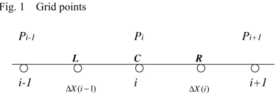
Eq.(32) is discretized by the central difference technique (Fig.1), i.e. ' ' ' 'P ₁ d P b P ₁ c a _i+ + _i + _i− = (35) where ) ( ) ( ' 3 i X n G a R ∆ = , ) 1 ( ) ( ' 3 − ∆ = i X n G b L , c'=(G1)R −(G1)L, d'=−a'−b'.

With the boundary conditions: P₁ =0 (at X=0), P_n+1 =0 (at X=1), Eq.(35) is solved

by the tri-diagonal matrix inverse.

Velocity distributions

The velocity distributions for sx =1, sy =0are

P C x x x u u b b h b z b h h z x p n u u b b h b z u u = + + + + + − ∂ ∂ + − + + + + = ( 2 )( )] 2 2 [ 1 1 ) ( 2 1 1 2 2 0 1 2 2 1 1 1 _µ (36)

if u1x =ub, and u2x =0, then Vx =−ub, and thus

] ) )( 2 ( 2 2 [ 1 1 ) ( 2 1 1 2 2 0 2 1 1 b b h b z b h h z x p n u b b h b z u u b b + + + + − ∂ ∂ + − + + + + = µ , (37) where 1 2 1 0 0 ) 1 ( − + + = n B B H η µ , 1 0 0 = ( ) − n b h u m η (38)

Eq. (37) is non-dimensionalized by ub, i.e. U =UP +UC

where 2 1 1 1 B B H B Z u u U b C C + + + − = = (39) 1 2 1 2 1 1 2 2 ) ]( ) )( 2 ( 2 2 [ 1 _{+ +} − + + + + + − ∂ ∂ − = = n b P P H B B B B H B Z B H H Z X P n u u U (40)

Results and Discussions

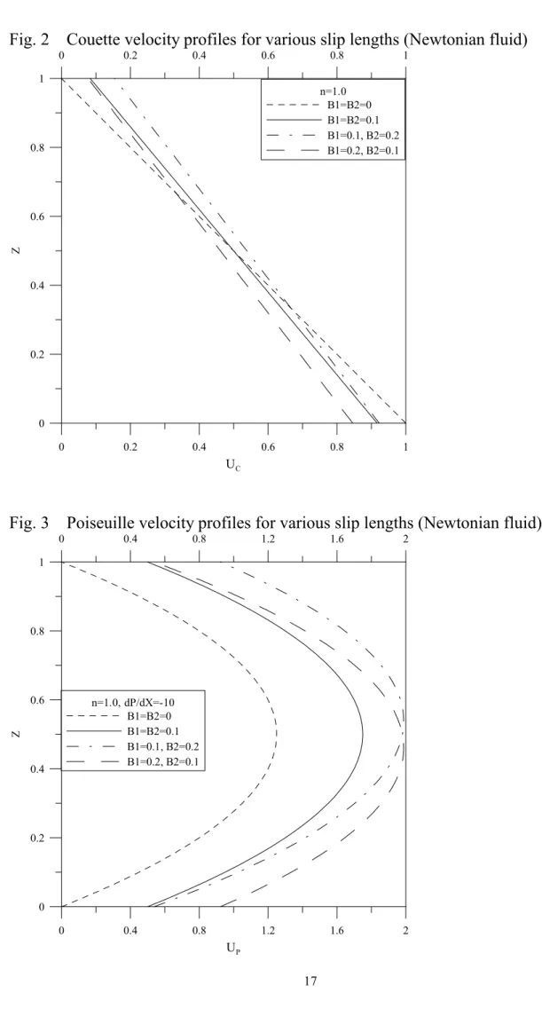
In the 1-D wedge problem, the upper plane is fixed and inclined, and the lower plane is moving with U=1. From Eq.(32), the pressure increases as the Poiseuille term (1G₃

n )

decreases, or as the Couette term (G₁) increases. As shown in Fig.2, the Couette flow for Newtonian fluid are plotted for four slip conditions, i.e. (B₁,B₂)= (0, 0), (0.1, 0.1), (0.1, 0.2), and (0.2, 0.1). The slip velocities on the boundaries are the same if

2 1 B

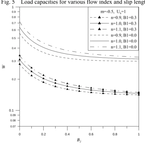
B = . The velocity profiles are parallel for the cases of (B₁,B₂)= (0.1, 0.2) and (0.2, 0.1). The Couette term for (B₁,B₂)=(0.1, 0.2) is greater than (B₁,B₂)=(0.2, 0.1). As shown in Fig.3, the Poiseuille flow for Newtonian fluid are plotted for four slip conditions, i.e. (B₁,B₂)= (0, 0), (0.1, 0.1), (0.1, 0.2), and (0.2, 0.1). The velocity profiles are not symmetric about the middle plane (Z=0.5) if B₁ ≠B₂. For the cases of (B₁,B₂)=(0.1, 0.2) and (B₁,B₂)= (0.2, 0.1), the velocity profiles are anti-symmetric about the middle plane (Z=0.5). The Poiseuille terms are the same for these two cases. Due to the contribution of Couette terms, the pressure distributions for

) ,

(B₁ B₂ =(0.1, 0.2) is greater than that for (B₁,B₂)= (0.2, 0.1), and thus we have the load capacity: W(0.1, 0.2)>W(0.2, 0.1).

In Fig.4, the Poiseuille flow are plotted for n=0.9, 1.0, 1.1. The Poiseuille term follows: shear thinning (n<1) > Newtonian (n=1) > shear thickening (n>1). Also, the larger the slip length, the larger the Poiseuille flow, thus the Poiseuille term follows

) ,

(B₁ B₂ =(0.3, 0.1) > (B₁,B₂)=(0.3, 0.3) > (B₁,B₂)=(0.3, 0.5). The slip lengths on moving boundary (B1) are the same, and the load capacities for larger B2 is smaller due to the less resistance. Larger slip length results in smaller resistance on Poiseuille flow, and thus results in smaller load capacities.

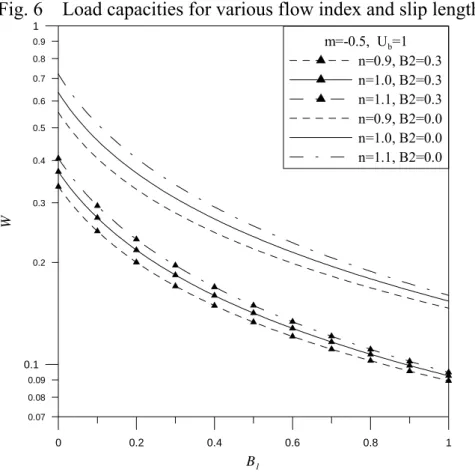
The load capacities for various flow indexes (n) are plotted as shown in Fig.5 and Fig.6. The load capacities follow: W(n<1)<W(n=1)<W(n>1), W(0,B₂)> W(0.3,B₂),

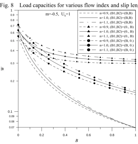
and W(B1, 0)> W(B1, 0.3). In Fig.7, the load capacities are plotted for various flow indexes and slip lengths (partially wetted). Three types of slip pairs are considered, i.e. (B₁,B₂)=(0.3, B), (B, 0.3), and (B, B). For B>0.3, we have W(0.3, B)>W(B, 0.3)>W(B, B). For B<0.3, we have W(0.3, B)<W(B, 0.3)<W(B, B). In Fig.8, one

lubricating surface follows the no-slip conditions. We have W(0, B)>W(B, 0)>W(B, B). From Fig. 7 and Fig. 8, the variation of load capacity with respect to the slip length,

B W

∂

∂ _{, is more sensitive for ( B, )}

B , i.e. ( , ) ( ,0.3) (0.3,B) B W B B W B B B W ∂ ∂ > ∂ ∂ > ∂ ∂ and ( , ) ( ,0) (0,B) B W B B W B B B W ∂ ∂ > ∂ ∂ > ∂ ∂ _. Conclusion

In this paper, the effects of slip velocity and flow rheology on the hydrodynamic pressure can be discussed from the derived extended Reynolds equation. The results show that smaller slip length on lubricating boundaries result in larger Couette term and smaller Poiseuille term, and thus result in larger hydrodynamic pressure. The load capacities follow: (1) effect of rheology: W(n<1)<W(n=1)<W(n>1), (2) effect of slip lengths: W(0,0)>W(BC,B) >W(B,BC) >W( BB, ) for B > BC , and W(0,0) >

) , ( BB

W >W(B,B_C)>W(B_C,B) for B< B_C, (3) sensitivity to slip length: ( BB, ) B W ∂ ∂ _> ) , (B BC B W ∂ ∂ _> ) , (B B B W C ∂ ∂ _. Acknowledgement

References

[1] Pit, R., Hervet, H., and Leger, L., 1999, “Friction and Slip of a Simple Liquid at a Solid Surface,” Tribology Letters, 7, pp.147-152.

[2] Pit, R., Hervet, H., and Leger, L., 2000, “Direct Evidence of Slip in Hexadecane: Solid Interfaces,” Phys. Rev. Letter, 85, pp.980-983.

[3] Zhu, Y., and Granick, S., 2001,” Rate dependent slip of Newtonian liquid at smooth surfaces,” Physics Review Letters, 87, 096105.

[4] Zhu, Y., and Granick, S., 2002,” Limits of hydrodynamic no-slip boundary condition,” Physics Review Letters, 88, 106102.

[5] Hild, W., Schaefer, J. A. and Scherge, M., 2002, “Microhydrodynamical studies of hydrophilic and hydrophobic surfaces” Proceedings of Thirteen International Colloquium on Tribology (Ed. W. J. Bartz), Esslingen, pp.821-825.

[6] Granick, S., Zhu, Y., and H. Lee, 2003, “Slippery Questions about complex fluids flowing past solids,” Nature Materials, Vol.2, pp.221-227.

[7] Thompson, P. A., and Robbins, M. O. 1990, “Shear flow near solids: epitaxial order and flow boundary condition,” Phys. Rev.A 41, 6830–6839.

[8] Thompson, P. A., and Troian, S.A, 1997, ”General boundary condition for liquid flow at solid surfaces,” Nature 389, 360–362.

[9] Barrat, J.-L., and Bocquet, L., 1999, “Large slip effect at a nonwetting fluid-solid interface,” Phys. Rev. Lett. 82, 4671–4674.

[10] Brenner, H., and Ganesan,V., 2000, “Molecular wall effects: are conditions at a boundary ‘boundary conditions’?” Phys. Rev. E. 61, 6879–6897.

[11] Gao, J., Luedtke,W. D., Landman,U. 2000, “Structures, solvation forces and shear of molecular films in a rough nano-confinement,” Tribol. Lett. 9,pp.133–134. [12] Denniston,C., and Robbins, M.O., 2001, “Molecular and continuum boundary

conditions for a miscible binary fluid,” Phys. Rev. Lett. 87, 178302.

[13] Campbell, S. E., Luengo, G., Srdanov,V. I.,Wudl, F., Israelachvili, J. N., 1996, “Very low viscosity at the solid-liquid interface induced by adsorbed C-60 monolayers. Nature 382, 520–522.

[14] Kiseleva,O. A., Sobolev,V. D., Churaev, N. V., 1999, “Slippage of the aqueous solutions of cetyltriimethylammonium bromide during flow in thin quartz capillaries,“ Colloid J. 61, 263–264.

[15] Craig,V. S. J.,Neto,C., Williams,D. R. M., 2001, “Shear-dependent boundary slip in aqueous Newtonian liquid,” Phys. Rev. Lett. 87, 54504.

[16] Zhu,Y., Granick, S., 2002, “Apparent slip of Newtonian fluids past adsorbed polymer layers,” Macromolecules 36, 4658–4663.

[17] Zhu,Y., Granick, S., 2002, “The no slip boundary condition switches to partial slip when the fluid contains surfactant,” Langmuir 18, 10058–10063.

boundary slip of water on hydrophilic surfaces and electrokinetic effects,” Phys. Rev. Lett. 88, 076103.

[19] Baudry, J.,Charlaix, E., Tonck, A., Mazuyer,D., 2002, “Experimental evidence of a large slip effect at a nonwetting fluid-solid interface,” Langmuir 17, 5232–5236. [20] Tretheway,D. C. & Meinhart, C. D., 2002, “Apparent fluid slip at hydrophobic

microchannel walls,” Phys. Fluids 14, L9–L12.

[21] Vinogradova,O. I., 1999, ”Slippage of water over hydrophobic surfaces,” Int. J. Miner. Process 56, 31–60.

[22] Cottin-Bizonne, C., Jurine, S., Baudry, J., Crassous, J., Restagno, F., and Charlaix, E., 2002, “Nanorheology: An Investigation of the Boundary Condition at Hydrophobic and Hydrophilic Interfaces,” The European Physical Journal E, Vol.9, pp.47-53.

[23] Spikes, H. A., 2003, "The Half-Wetted Bearing. Part 1: Extended Reynolds Equation," IMechE, Part J, J. Engineering Tribology, 217, pp.1-14.

[24] Spikes, H. A., 2003, "The Half-Wetted Bearing. Part 2: Potential Application in Low Load Contacts," IMechE, Part J, J. Engineering Tribology, 217, pp.15-26. [25] Dien, I. K., and Elrod, H. G., 1983, “A generalized steady-state Reynolds equation

for non-Newtonian fluids, with application to journal bearings,” ASME J. Lubrication Technology, 105, 385-390.

Nomenclature

b = the slip length i

B = non dimensional slip length, =b_i / h₀ h = film thickness

H = non dimensional film thickness, =h/ h₀

0

h = film thickness at the leading edge

I = the second invariant of the strain rate tensor 0

I = zero order component of I

1

I = first order component of I l = slider length

m = slope of the wedge

n = flow index of power law fluid p = pressure

P = non dimensional pressure,

l u ph b 0 2 0 η = u = the velocity in the x-direction

0

u = zero order velocity component in x-direction

1

u = first order velocity component in x-direction b

u = boundary velocity of 1-D wedge problem

ix

u = translational velocity of i-th surface in x-direction

v = the velocity in the y-direction 0

v = zero order velocity component in y-direction

1

v = first order velocity component in y-direction iy

v = translational velocity of i-th surface in y-direction

s

v = the slip velocity

i

V = the slide surface velocity in i- direction

W = load capacity X = x / l ε = small parameter 0 η = reference viscosity, 1 0 ) ( − = b n h u m µ = viscosity 0

µ = zero order component of µ 1

µ = first order component of µ s

σ = shear stress at the surface, zx

Figure Legends

Fig. 1 Grid points

Fig. 2 Couette velocity profiles for various slip lengths (Newtonian fluid) Fig. 3 Poiseuille velocity profiles for various slip lengths (Newtonian fluid) Fig. 4 Poiseuille velocity profiles for various flow index

Fig. 5 Load capacities for various flow index and slip lengths (fixed surface) Fig. 6 Load capacities for various flow index and slip lengths (moving surface) Fig. 7 Load capacities for various flow index and slip lengths

Fig. 1 Grid points

i i+1

i-1

P

P

P

Fig. 2 Couette velocity profiles for various slip lengths (Newtonian fluid) 0 0.2 0.4 0.6 0.8 1 U_C 0 0.2 0.4 0.6 0.8 1 Z 0 0.2 0.4 0.6 0.8 1 n=1.0 B1=B2=0 B1=B2=0.1 B1=0.1, B2=0.2 B1=0.2, B2=0.1

Fig. 3 Poiseuille velocity profiles for various slip lengths (Newtonian fluid)

0 0.4 0.8 1.2 1.6 2 UP 0 0.2 0.4 0.6 0.8 1 Z 0 0.4 0.8 1.2 1.6 2 n=1.0, dP/dX=-10 B1=B2=0 B1=B2=0.1 B1=0.1, B2=0.2 B1=0.2, B2=0.1

Fig. 4 Poiseuille velocity profiles for various flow index 0 0.1 0.2 0.3 0.4 U_P/(-dP/dX) 0 0.2 0.4 0.6 0.8 1 Ζ n=0.9 n=1.0 n=1.1 B2=0.1 B2=0.5 B₁=0.3

Fig. 5 Load capacities for various flow index and slip lengths (fixed surface)

0 0.2 0.4 0.6 0.8 1 B₂ 0.1 1 0.2 0.3 0.4 0.5 0.6 0.7 0.8 0.9 0.09 0.08 0.07 W m=-0.5, U_b=1 n=0.9, B1=0.3 n=1.0, B1=0.3 n=1.1, B1=0.3 n=0.9, B1=0.0 n=1.0, B1=0.0 n=1.1, B1=0.0

Fig. 6 Load capacities for various flow index and slip lengths (moving surface) 0 0.2 0.4 0.6 0.8 1 B₁ 0.1 1 0.2 0.3 0.4 0.5 0.6 0.7 0.8 0.9 0.09 0.08 0.07 W m=-0.5, Ub=1 n=0.9, B2=0.3 n=1.0, B2=0.3 n=1.1, B2=0.3 n=0.9, B2=0.0 n=1.0, B2=0.0 n=1.1, B2=0.0

Fig. 7 Load capacities for various flow index and slip lengths

0 0.2 0.4 0.6 0.8 1 B 0.1 0.2 0.3 0.4 0.5 0.6 0.7 0.09 0.08 0.07 W n=0.9, (B1,B2)=(B,B) n=1.0, (B1,B2)=(B,B) n=1.1, (B1,B2)=(B,B) n=0.9, (B1,B2)=(0.3, B) n=1.0, (B1,B2)=(0.3, B) n=1.1, (B1,B2)=(0.3, B) n=0.9, (B1,B2)=(B, 0.3) n=1.0, (B1,B2)=(B, 0.3) n=1.1, (B1,B2)=(B, 0.3) m=-0.5, U_b=1

Fig. 8 Load capacities for various flow index and slip lengths 0 0.2 0.4 0.6 0.8 1 B 0.1 1 0.2 0.3 0.4 0.5 0.6 0.7 0.8 0.9 0.09 0.08 0.07 W n=0.9, (B1,B2)=(B,B) n=1.0, (B1,B2)=(B,B) n=1.1, (B1,B2)=(B,B) n=0.9, (B1,B2)=(0., B) n=1.0, (B1,B2)=(0., B) n=1.1, (B1,B2)=(0., B) n=0.9, (B1,B2)=(B, 0.) n=1.0, (B1,B2)=(B, 0.) n=1.1, (B1,B2)=(B, 0.) m=-0.5, U_b=1