非同步約分諧波鎖模掺鉺光纖光固子雷射之雷射動力學

國 立 交 通 大 學

顯 示 工 程 研 究 所

碩士論文

非同步約分諧波鎖模掺鉺光纖光固子雷射

之雷射動力學

Laser dynamics of asynchronous rational

harmonic mode-locked Er-doped fiber soliton

laser

研究生 : 江國豪

指導教授 : 賴暎杰 博士

I

非同步約分諧波鎖模掺鉺光纖光固子雷射

之雷射動力學

研究生:江國豪 教授:賴暎杰 博士

國立交通大學顯示工程研究所

摘要

本論文主要探討非同步約分諧波鎖模掺鉺光纖光固子雷射的雷 射動力學特性，一方面透過約分諧波鎖模來達到超高重複率，也同時 透過非同步鎖模來獲得良好的鎖模脈衝輸出。我們在實驗上進一步利 用非同步鎖差頻的方式來補償共振腔的擾動，接著量測和探討整個雷 射系統的雷射動力學。我們也利用 RF 頻譜的資訊計算出非同步約分 諧波鎖模脈衝在時間上的變化和光頻的變化，利用這些結果去反推等 效調變深度，並進一步驗證相位調變非同步約分諧波鎖模雷射的等效 調變效應主要來源為 RF 放大器的高階分量。我們在探討雷射動力學 的時候也發現了一個新的同步諧波鎖模雷射操作模態，可以產生重複 率高達 40GHz 的穩定鎖模脈衝雷射並在 RF 頻譜觀察到邊頻項，透過 設計一連串的實驗我們也探討了這個有趣新穎的新操作模態。

II

Laser dynamics of asynchronous rational

harmonic mode-locked Er-doped fiber

soliton laser

Student: Guo-Hao Jiang Advisor: Dr. Yinchieh Lai

Institude of Display, National Chiao-Tung University

Abstract

The thesis is focused on the laser dynamics studies of asynchronous rational harmonic mode-locked Er-doped fiber soliton lasers. The rational harmonic mode-locking can provide higher repetition rates and the asynchronous mode-locking can help achieve good mode-locking performance. We stabilize the laser cavity length by locking the deviation frequency of asynchronous mode-locking to help measure the laser dynamics of the laser system. Base on the information of the RF spectra, we estimate the timing and center frequency variation of the asynchronous rational harmonic mode-locked pulse trains. We verify that the effective modulation strength is mainly from the higher order signals of the RF amplifier in asynchronous rational harmonic mode-locked lasers with only phase modulation. We also experimentally find a new

III

operation state of synchronous harmonic mode-locking. Stable 40 GHz mode-locking operation can be achieved with RF spectral sidebands quite similar to the asynchronous mode-locking. A series of experiments have been performed to investigate the characteristics of this interesting new operation state.

IV

誌謝

在實驗室短短的兩年裡因為實驗上的需要學習到好多知識和解 決問題的能力，雖然實驗中遇到許多不可預期的困難，但最後都一一 解決了，現在要和實驗室的大家說再見並感謝大家一路的幫助。 首先要感謝的是我的指導教授賴暎杰，老師在我有問題的時候總 是很有耐性的跟我解釋，這些問題並不侷限在專業的知識上，在我徬 徨無助的人生路上，老師也能給予我適當的建議以及不同的想法，帶 著老師所指導的一切離開學校我覺得心滿意足，在未來的日子裡一定 不負老師的教誨一步一步實踐我的夢想。 感謝實驗室實力堅強的學長姊們：鞠曉山學長、項維巍學長、徐 桂珠學姊、許萓蘘學姊、吳尚穎學長、王聖閔學長不僅教會我使用儀 器的方法還有解釋實驗數據的方式，你們許多寶貴的意見學弟我都有 聽到並吸收，這些珍貴的經驗傳授讓我能更快達到實驗的目標。 也要感謝實驗室的夥伴們，楊良愉、林仕斌、黃耀德、顧戎，實 驗室有你們的陪伴樂趣增加不少，在我因為實驗不順利心情不好時你 們陪我聊天陪我玩 LOL(英雄聯盟)舒緩我的壓力，讓我更有動力面對 接下來的問題。 最後要感謝我的家人還有我的女朋友洪詩婷，在我努力認真求學 的階段裡一直陪伴著我。

V

Contents

Chinese Abstract...I

English Abstract...II

Acknowledgements...III

Contents...IV

List of Figures...VII

Chapter 1: Introduction

1.1 Overview...1

1.2 Motivation of the research...4

1.3 Organization of the thesis...5

References...6

Chapter 2:

Principles

of mode-locked fiber lasers

2.1 Active mode-locking………...…………7

2.1.1 Amplitude modulation mode-locking…………8

2.1.2 Phase modulation mode-locking………..11

2.2 Rational harmonic mode-locked fiber laser…………..13

2.3 Asynchronously mode-locked (ASM) fiber laser…….18

2.4 Long-term stabilization of mode-locked fiber laser…..21

VI

Chapter 3: Experimental setup and results

3.1 21GHz asynchronous rational harmonic mode-locked (ARHM) Er-fiber soliton laser with stabilization

3.1.1 Experimental setup and component parameters ………...30 3.1.2 Experimental results………33 3.2 Pulse dynamics of ARHM fiber soliton laser

3.2.1 Periodic pulse timing position and center frequency variation………..38

3.2.2 Determination of the effective modulation depth……….45

3.3 33 GHz asynchronous rational harmonic mode-locked Er-fiber soliton laser……….51

3.4 New state of synchronous harmonic mode-locking…..54

References………68

Chapter 4: Conclusions

4.1 Summary of achievements………70 4.2 Future work………...72

VII

List of Figures

Fig. 2.1 Schematic of an active mode-locked laser ... 7

Fig. 2.2 Actively mode-locked modes in the frequency domain ... 8

Fig. 2.3 Diagram of the amplitude modulation mode-locking in the frequency domain. ... 9

Fig. 2.4 Actively mode-locked pulses in the time domain and the time dependence of the net gain. ... 10

Fig. 2.5 Formulation of pulse trains in the time domain. ... 12

Fig. 2.6. Sketch of light modulation in the cavity after T, 2T, 3T, 4T respectively ... 15

Fig. 2.7 (a) Pulse train in the particular position of time domain. (b) Pulse in the modulation transmission curve at immediate time ... 16

Fig. 2.8 Laser cavity with the gain, filter, group velocity dispersion (GVD), self phase modulation(SPM) and the phase modulation driven asynchronously. ... 18

Fig.2.9 The noise-cleanup effect in the asynchronous mode-locked soliton laser. ... 19

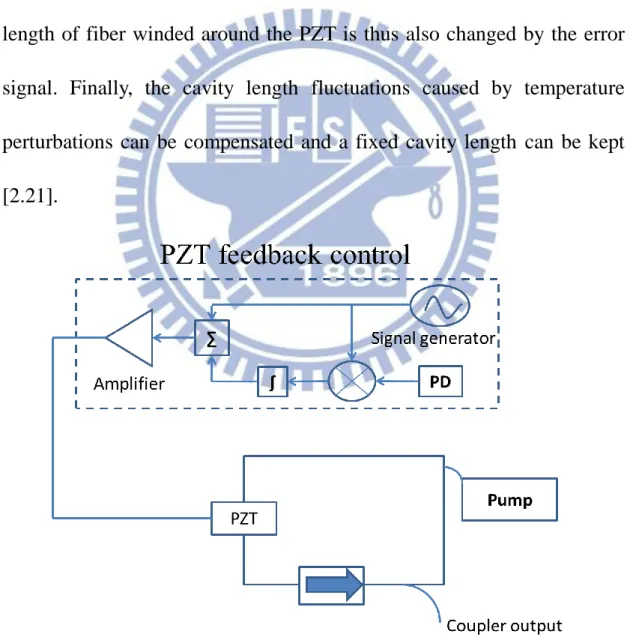
Fig. 2.10 Schematic setup of PZT feedback control ... 22

Fig. 2.11 Diagram of regenerative mode-locked fiber laser ... 23

Fig. 3.1 The experimental setup ... 30

Fig. 3.2 RF spectrum of laser output near 21 GHz with 40 GHz span ... 34

VIII

Fig. 3.4 RF spectrum of laser output near 21 GHz with 500 kHz span ... 35

Fig. 3.5 Optical spectrum of the 21GHz rational asynchronous mode-locked Er-fiber soliton laser ... 35

Fig. 3.6 SHG intensity autocorrelation trace (open circles) and the fitting curve (solid curve) of the laser output, assuming sech2 pulse shape. ... 36

Fig. 3.7 Deviation frequency shift: without the stabilization scheme (red dash line); with the stabilization scheme (black solid line). ... 37

Fig. 3.8 RF spectrum at 21 GHz with 0 m SMF 28 fiber ... 41

Fig. 3.9 RF spectrum at 21 GHz with 200 m SMF 28 fiber ... 41

Fig. 3.10 RF spectrum near 21 GHz with 300 m SMF 28 fiber ... 42

Fig. 3.11 RF spectrum near 21 GHz with 500 m SMF 28 fiber ... 42

Fig. 3.12 Measurement of the net pulse timing variation versus the length of the SMF-28 fiber. ... 43

Fig. 3.13 RF spectrum at 21 GHz with 0 m SMF 28 fiber ... 46

Fig. 3.14 SHG intensity autocorrelation trace (open circles) and the fitting curve (solid curve) of the laser output, assuming sech2 pulse shape. ... 46

Fig. 3.15 RF spectrum at 21 GHz with 0 m SMF 28 fiber ... 48

Fig. 3.16 SHG intensity autocorrelation trace (open circles) and the fitting curve (solid curve) of the laser output, assuming sech2 pulse shape. ... 48

IX

Fig. 3.17 RF spectrum of laser output near 33 GHz with 40 GHz span ... 51

Fig. 3.18 RF spectrum of laser output near 33 GHz with 50 MHz span ... 52

Fig. 3.19 RF spectrum of laser output near 33 GHz with 500 kHz span ... 52

Fig. 3.20 Optical spectrum of the 33GHz asynchronous rational mode-locked Er-fiber soliton laser ... 53

Fig. 3.21 SHG intensity autocorrelation trace (open circles) and the fitting curve (solid curve) of the laser output, assuming sech2 pulse shape. ... 53

Fig. 3.22 RF spectrum at 40 GHz in with 500 kHz span ... 55

Fig. 3.23 RF spectrum at 40 GHz with 50 MHz span and SMSR > 55 dB ... 56

Fig. 3.24 SHG intensity autocorrelation trace (open circles) and the fitting curve (solid curve) of the laser output, assuming sech2 pulse shape. ... 56

Fig. 3.25 Optical spectrum of the 40GHz harmonic mode-locked Er-fiber soliton laser ... 57

Fig. 3.26 The deviation frequency shift with duration time of stabilization ... 57

Fig. 3.27 RF spectrum at near 40 GHz with 40 GHz span ... 58

Fig. 3.28 RF spectrum at near 40 GHz in with 500 kHz span ... 59

Fig. 3.29 RF spectrum at near 40 GHz with 50 MHz span and SMSR ≈ 60 dB ... 59

Fig. 3.30 SHG intensity autocorrelation trace (open circles) and the fitting curve (solid curve) of the laser output, assuming sech2 pulse shape. ... 60

X

Fig. 3.31 Optical spectrum of the 40GHz rational harmonic mode-locked Er-fiber soliton laser ... 60 Fig. 3.32 Low frequency spectrum of the output pulse train. Large deviation

frequency situation (red dash line), synchronous situation (blue dot line) and no modulation signal situation (black solid line). ... 61 Fig. 3.33 Linear relation between the optical power of the autocorrelator port and the

deviation frequency of the spectral side peaks. ... 62 Fig. 3.34(a) RF spectrum in synchronous mode-locking at near 20 GHz with 500 kHz

span ... 64 Fig. 3.34(b) Synchronous mode-locked pulse trains by the fast sampling oscilloscope

... 64 Fig. 3.35(a) RF spectrum in asynchronous mode-locking at near 20 GHz with 500

kHz span ... 65 Fig. 3.35(b) Asynchronous mode-locked pulse trains by the fast sampling oscilloscope

... 65 Fig. 3.36(a) RF spectrum in large deviation frequency mode-locking at near 20 GHz

with 500 kHz span ... 66 Fig. 3.36(b) Large deviation frequency mode-locked pulse trains by the fast sampling

1

Chapter 1

Introduction

1.1 Overview

A fiber laser is a laser in which the gain medium is an optical fiber doped with rare-earth elements such as erbium (1550nm) and ytterbium (1060nm). The 1550nm wavelength region has the lowest fiber propagation loss and has been widely utilized as the fiber communication spectral window. Because of this, the erbium-doped fiber laser is most suitable for optical communication purposes and has also been popularly applied in the measurement equipment. In contrast, the ytterbium-doped fiber laser is most suitable for industrial applications due to the achievable high output power and conversion efficiency.

According to the gain medium type, we can classify lasers into categories of gas, liquid, and solid state. Gas state laser like CO2 laser can be applied for many applications required high power. Semiconductor laser is one of the most common types of solid state lasers. It is suitable to be integrated with electrical devices due to their electrical pumping characteristics. However, for generating ultrashort optical pulses, the mode-locked fiber laser would be more suitable than many other lasers

2

due to the large gain bandwidth of rare-earth-doped fibers, which is essential for producing ultrashort pulses. Ultrashort pulse can help avoid organism tissue damage resulted from the heat heap. Because of this, ultrashort pulse laser is also popularly applied in the area of biophotonics.

Typically there are two ways to achieve mode-locking of the lasers. One is the passive mode-locking and the other is the active mode-locking. The passive mode-locking can generate shorter pulses than active mode-locking while the active mode-locking can generate higher repetition rates than the passive mode-locking. One can also employ hybrid mode-locking which contains these two mode-locking mechanisms to generate ultrashort pulse trains in the high repetition rates. However, in practice there are still many other problems needed to be solved. One of the most important issues is the environmental perturbation resulted from the effects of expanding when hot and shrinking when cold. This effect apparently influences the stability of active mode-locked fiber lasers due to the cavity length variation caused by environmental temperature perturbation, because in general, active mode-locking is possible only when the modulation frequency and the harmonic mode frequency in the cavity can synchronize. Since it is not

3

practical to set up systems in the experimental environments without perturbations, it is thus crucial to know how to employ a feedback control loop to compensate the cavity length variation.

In the past literature, many methods have been used to help maintain the pulse train of high repetition rates in mode-locked fiber lasers. By installing an optical etalon in the laser cavity, a regenerative mode-locked fiber laser can achieve mode-hop-free operation [1.1]. Another economic way is to employ asynchronous mode-locking scheme. The feedback stabilization control can be achieved by detecting the deviation frequency between the modulation frequency of phase modulation and the harmonic frequency of the cavity. In this way the error signal can be utilized to control the optical delay line to correct the cavity length for laser stabilization..

Recently, asynchronous mode-locked Er-doped fiber soliton laser has been investigated extensively. Direct generating of 10GHz 816 fs pulse train from an erbium-fiber soliton mode-locked fiber laser with asynchronous phase modulation has been demonstrated [1.2]. Applying asynchronous mechanism to stabilize high repetition rate fiber lasers for long time operation has also been successfully demonstrated [1.3]. Even

4

though harmonic mode-locking can generate high repetition rate pulse trains, it is still limited by the available modulation frequency. It will be nice to have some other methods to increase the repetition rate. One of these methods is to employ the rational harmonic mode-locked mechanism by detuning the modulation frequency with a rational order of the fundamental frequency of the cavity [1.4]. This kind of high repetition rate mode-locked fiber lasers that can output ultrashort pulse trains is suitable for high speed optical communication and ultrafast optical signal processing [1.5].

1.2 Motivation

Asynchronous mode-locked fiber soliton lasers have been attractive due to the low cost stabilization method and the high supermode suppression ratio (SMSR). It is natural to expect that by combining the asynchronous mode-locking mechanism and the rational harmonica mode-locking mechanism, one may be able to generate high repetition rate pulse trains without being limited by the synthesizer frequency and without suffering from the environmental perturbations. However, the laser dynamics of asynchronous rational harmonic mode-locked Er-doped

5

fiber soliton lasers have not been well studied. It will be important to understand more about their laser dynamics before one can actually develop their applications.

1.3 Organization of this thesis

This thesis consists of four chapters. Chapter 1 is an overview of the fiber laser development and the motivation for carrying out this research. Chapter 2 describes the methods of active mode-lockingand discusses the issues of rational harmonic mode-locking, asynchronous mode-locking, and long-term stabilization of mode-locked fiber lasers. Chapter 3 presents the experimental setup and analyzes the results of experiments. Finally, Chapter 4 gives a summary about our achievements and possible future work.

6

Reference

[1.1] M. Yoshida, K. Kasai and M. Nakazawa, “Mode-hop-free optical frequency tunable 40 GHz mode-locked fiber laser,” IEEE J. Quantum Electron. 8, 704 (2007).

[1.2] W. W. Hsiang, C. Y. Lin, M. F. Then and Y. Lai, “Direct generation of a 10 GHz 816 fs pulse train from an erbium-fiber soliton laser with asynchronous phase modulation,” Opt. Lett. 18, 2493 (2005).

[1.3] W. W. Hsiang, C. Y. Lin, N. Sooi and Y. Lai, “Long-term stabilization of a 10 GHz 0.8 ps asynchronously mode-locked Er-fiber soliton laser by deviation-frequency locking,” Opt. Express 5, 1822 (2006).

[1.4] C. Wu and N. K. Dutta, “High-repetition-rate optical pulse generation using high-repetition-rate optical pulse generation using,” IEEE J. Quantum Electron. 2, 145 (2000).

[1.5] J. P. Wang, B. S. Robinson, S. A. Hamilton, and E. P. Ippen, “Demonstration of 40-Gb/s packet routing using all-optical header processing,” IEEE Photon. Technol. Lett. 21, 2275 (2006).

7

Chapter 2

Theories of mode-locked fiber lasers

2.1 Active mode-locking

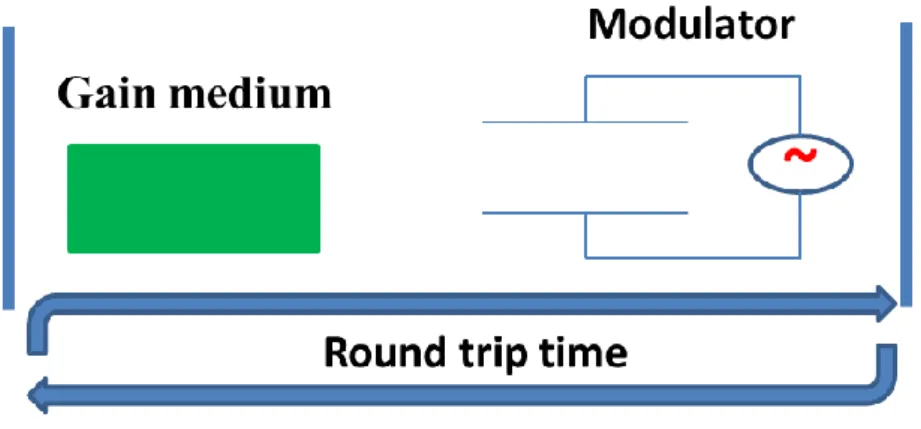
The active mode-locking mechanism is based on the active modulation which induces the loss or phase modulation in the laser cavity. The utilized active modulators may be either the acousto-optic or the electro-optic modulators. If the modulation frequency is synchronized with the resonator round trip time, the optical pulse trains in the cavity will continue to grow and finally achieve stable mode-locking (Fig. 2.1). In general, active mode-locked fiber lasers can use two different methods for optical modulation. One is the amplitude modulation (AM) mode-locking, and the other is the phase modulation (PM) mode-locking. Detailed introduction for the two general methods of modulation will be given in the following section.

8

2.1.1 Amplitude modulation mode-locking

Amplitude modulation mode-locking is a way in which the optical amplitude is modulated directly to produce a short pulse train. This mechanism can be analyzed both in the frequency domain and the time domain [2.1].

In frequency domain, as the net gain of the system is greater than zero, longitudinal modes will start to lase. The longitudinal modes are separated equally in the frequency domain and the frequency interval is , where is the round trip time. Denoting the center frequency to be , the sidebands which center on will grow together as explained below if the lasers carry out mode-locking by the method of amplitude modulation.

9

Assuming the optical signal in the resonator is , then the amplitude modulated optical signal can be expressed as below:

(2-1)

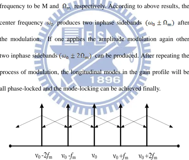
Here we have denoted the modulation depth and modulation frequency to be M and respectively. According to above results, the center frequency produces two inphase sidebands after the modulation. If one applies the amplitude modulation again other two inphase sidebands can be produced. After repeating the process of modulation, the longitudinal modes in the gain profile will be all phase-locked and the mode-locking can be achieved finally.

ν

0

-2f

m

ν

0

-f

m

ν

0

ν

0

+f

m

ν

0

+2f

m

Fig. 2.3 Diagram of the amplitude modulation mode-locking in the frequency domain.

In the time domain analysis, the modulator produces a periodic loss in the cavity. Pulse trains builds up when the gain is greater than the

10

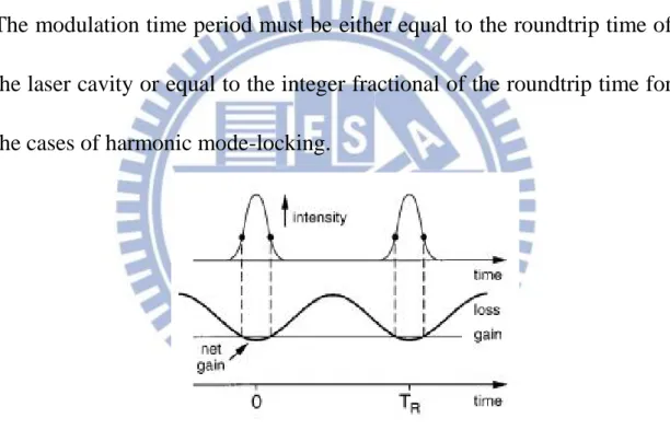
loss. If the optical signal passes through the maximum transmission point every roundtrip, then the optical signal will be amplified again and again until it reaches the steady state. The pulsewidth become shorter after passing through the amplitude modulator repeatedly. The pulse shortening strength caused by modulation balances the pulse broadening strength caused by the dispersion/filtering effects of the cavity in the steady state. The modulation time period must be either equal to the roundtrip time of the laser cavity or equal to the integer fractional of the roundtrip time for the cases of harmonic mode-locking.

Fig. 2.4 Actively mode-locked pulses in the time domain and the time dependence of the net gain.

The master equation of amplitude modulation mode-locked lasers can be written as:

11

where g is the gain per pass, l is the loss, is the gain bandwidth and M is the modulation index.

2.1.2 Phase modulation mode-locking

Phase modulation mode-locking is a way in which the optical signal is phase modulated directly to produce short pulse trains. This mechanism again can be analyzed both in the frequency domain and the time domain.

In the frequency domain, we assume the center frequency is as before. When the longitudinal mode is modulated by passing through the phase modulator, the optical signal can be written as below:

(2-3)

(2-4)

where M is the modulation index, is the modulation frequency and is the n-th order Bessel function.

It can be seen that the optical signal consist of unlimited sidebands when (2-3) is expanded into (2-4). The periodic pulse trains are formed when the phases of different modes are mode-locked. The pulse trains diagram is shown in Fig. 2.5

12

Fig. 2.5 Formulation of pulse trains in the time domain.

In the time domain, the phase of the optical pulse will be changed by the phase modulator. In the beginning, we can set the constant phase without modulation effect is . Then the optical phase changed by the phase modulator can be expressed by a Taylor series and the result is written as below:

+… (2-5)

where means the immediate frequency. When , the modulation will cause the frequency shift of the optical pulse. Central frequency will continue to be shifted when passing through the phase modulator per round trip, until the optical pulse is shifted out of the gain bandwidth and disappears. As a result, only the synchronized pulses can survive in the laser cavity and then reach the steady state. However, has two solutions (positive 2nd order derivative and negative 2nd order derivative). There will be only one stable solution depending on the

13

sign of and the sign of the cavity dispersion.

2.2 Rational Harmonic mode-locked fiber laser

The high repetition rate mode-locked fiber laser may be useful for high bit rate optical communication systems. The active mode-locking of Er-doped fiber lasers is an attractive way for achieving mode-locking because it can offer transform-limited, sub-picosecond pulse trains with a repetition rate of 10 GHz or higher [2.2] [2.3]. However, the repetition rate of fiber laser is limited by the bandwidths of the electro-optic modulator, synthesizer and RF power amplifier. Rational harmonic mode-locked (RHML) technique can overcome this problem and thus it has attracted a great deal of interest. The method is to detune the modulation frequency away from the longitudinal mode of harmonic mode-locking (HML) to generate high repetition rate pulse trains [2.4].

In this mode-locked mechanism, the final repetition rate can be

(2-6)

when the modulation frequency is set at

(2-7)

14

(2-8)

Here n and p are integrals, c is the optical speed in the vacuum and is the effective index of the cavity and L is the cavity length.

By using the RHML laser configuration, Nakazawa and Yoshida have achieved high repetition rate rational harmonic mode-locked fiber laser up to 80-200GHz [2.5]. L. R. Chen hasdemonstrated wavelength-tunable, 30-GHz pulse train generation from a rational harmonic mode-locked fiber optical parametric oscillator (FOPO) by using a 10-GHz driving source [2.6].

If the fiber laser is applied to practical systems, the stability of the optical pulse trains from a fiber laser needs to be improved. The instability may originally come from three main causes:

1) Polarization fluctuations in the long fiber cavity due to fiber vibrations,

2) Cavity length drifts due to the temperature fluctuations.

3) Supermode noises which frequencies could be any integral multiples of the cavity fundamental frequency.

Several approaches have been developed to overcome these problems. Nakazawa and Yoshida constructed the fiber lasers with an

15

all-polarization-maintaining ring cavity [2.3] [2.7]. The issues about how to stabilize the fiber cavity length from not being suffered from the fluctuations in the temperature will be given in Chapter 2.4.

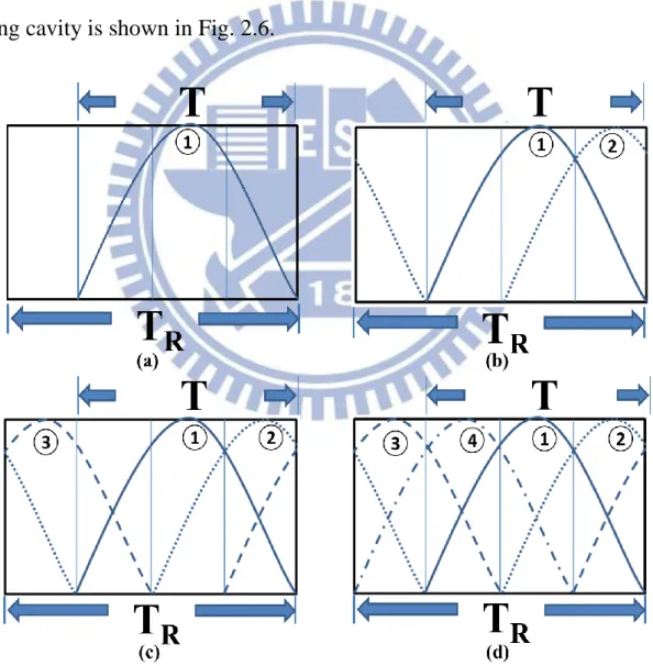
However, the most important problem in the rational harmonic mode-locking is the pulse amplitude variation. Considering a simple example when , the diagram of light modulation in the ring cavity is shown in Fig. 2.6.

Fig. 2.6. Sketch of light modulation in the cavity after T, 2T, 3T, 4T respectively

16

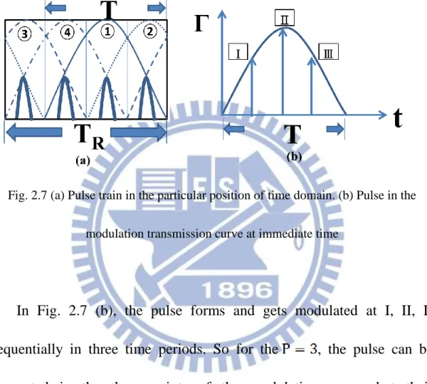
this process will continue to go through repeatedly. The lights in the cavity are amplified and eventually form the pulse trains in the particular position of time domain as shown in the Fig. 2.7 (a).

Fig. 2.7 (a) Pulse train in the particular position of time domain. (b) Pulse in the modulation transmission curve at immediate time

In Fig. 2.7 (b), the pulse forms and gets modulated at I, II, II sequentially in three time periods. So for the , the pulse can be generated in the three points of the modulation curve, but their transmission ratios are different in different time periods. That is the reason why the amplitude variation usually occurs in the rational harmonic mode-locked fiber lasers.

To solve this problem, several researches have been reported for amplitude equalization. By properly adjusting the bias level of the

17

modulator one can equalize the amplitude [2.8]. N.K. Dutta has applied this equalized technique to demonstrate a rational harmonic mode-locked fiber laser with amplitude-equalized output operating at 80 Gbits/s [2.9]. Another main technique for equalizing the pulse amplitude is by using the SOA [2.10].

Rational harmonic mode-locking can be carried out by an amplitude modulator or a phase modulator [2.11]. X. Bao gave a conclusion that rational harmonic mode-locking can be achieved by using the phase modulation and better performance than the counterpart with amplitude modulation can be expected [2.12].

18

2.3 Asynchronously mode-locked fiber laser

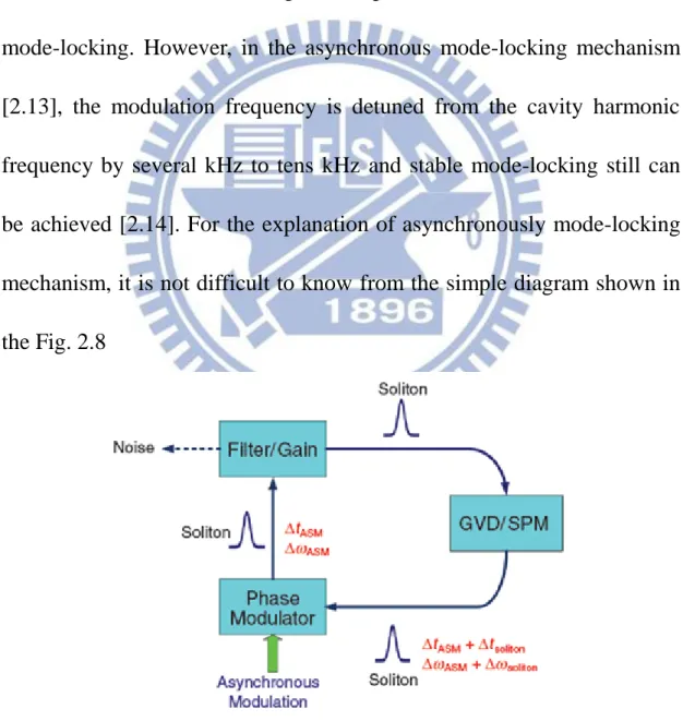
In active harmonic mode-locked lasers, the modulation frequency must exactly be equal to the cavity harmonic frequency, since otherwise the pulse trains cannot build up in the cavity. This is because the optical pulses will be shifted by a frequency if not synchronized. In the presence of finite bandwidth filter and gain, the pulse train cannot achieve stable mode-locking. However, in the asynchronous mode-locking mechanism [2.13], the modulation frequency is detuned from the cavity harmonic frequency by several kHz to tens kHz and stable mode-locking still can be achieved [2.14]. For the explanation of asynchronously mode-locking mechanism, it is not difficult to know from the simple diagram shown in the Fig. 2.8

19

modulation (SPM) and the phase modulation driven asynchronously.

The fiber laser of Fig. 2.8 is consisted of the optical bandpass filter, group velocity dispersion (GVD), self phase modulation (SPM), gain medium and the phase modulator. Under this laser configuration, the pulse does not disappear in the cavity. On the contrary, stable pulse trains can be realized and compressed to sub-picosecond pulse-width with the 10GHz repetition rate [2.15]. The noise clean up mechanism is similar to the effects of sliding-frequency guiding filters in soliton communication systems [2.16]. The soliton effects induced by the fiber nonlinearity in the asynchronous mode-locked fiber laser can help the mode-locked pulses to survive the asynchronous phase modulation. As a result, the solitons can exist steadily in the cavity, as is shown in Fig. 2.9.

Fig.2.9 The noise-cleanup effect in the asynchronous mode-locked soliton laser.

20

propagation, but the central frequency of the linear noises keep fixed and will be filtered out by the optical filter. So the asynchronous mode-locking mechanism can provide high SMSR performance without requiring additional intracavity optical devices [2.17].

Applying asynchronous mode-locking in fiber lasers to generate ultra-short pulses provides other advantages. One is to utilize the deviation frequency for feedback use. The other is to take advantages of the laser dynamics of asynchronous mode-locked fiber lasers for special applications [2.18]. These two aspects will be discussed in Chapter 2.4 and Chapter 3.

21

2.4 Long-Term Stabilization of Mode-Locked fiber

laser

The generation of ultrashort optical pulses in the GHz level is very important for high bit rate optical communication and optical metrology [2.19]. The most common way to produce high speed optical pulse trains is through active mode-locking. In the literature, many techniques have been carried out. These techniques include synchronous mode-locking, asynchronous mode-locking, rational harmonic mode-locking and regenerative mode-locking [2.20].

When the laser speed is improved to the GHz level, applications in practical systems still require enhancing the stability of optical pulse trains. There are many researches to reduce the noises for achieving long-term stabilization of the mode-locked fiber laser. They are as given in the below:

A) PZT

The main cause for laser instability is the cavity length drift due to the temperature fluctuations. This perturbation causes the repetition rate to shift and then the mode-locking cannot be maintained. The supermodes may also oscillate simultaneously and compete with each other. Thus the

22

fluctuations of pulse amplitude are generated, which appear as noises in the RF spectrum.

As said above, controlling the cavity length is a direct way to enhance the stability. It can use the error signal from the mixing of the modulation frequency signal and the pulse repetition rate signal to control the voltage of PZT. The PZT is lengthened or shorted by the applied voltage. The length of fiber winded around the PZT is thus also changed by the error signal. Finally, the cavity length fluctuations caused by temperature perturbations can be compensated and a fixed cavity length can be kept [2.21].

23

B) Regenerative mode-locking [2.3]

As shown in Fig. 2.11, the 40GHz clock extraction circuit is used to extract the 40 GHz clock from the laser output. The clock is then amplified and applied to the phase modulator. Finally, mode-locking is carried out. The laser operation continued stably for a long time because the modulation frequency (i.e. clock signal) always follows the changes in the cavity length. This means the modulation frequency and the cavity harmonic frequency always keep synchronous.

Fig. 2.11 Diagram of regenerative mode-locked fiber laser

Recently, the mode-locked fiber laser stabilization techniques are improved to a more advanced level. Base on the regenerative

24

mode-locked technique, Nakazawa and Yoshida have successfully demonstrated the mode-hop-free optical frequency tunable mode-locked fiber laser [2.22].The wavelength reference of C2H2 is employed to absolutely stabilize the optical frequency of the mode-locked fiber laser [2.23]. It is also possible to independently stabilize the repetition rate and the optical frequency [2.24].

Base on controlling the cavity length to lock the deviation frequency at a suitable value, there is a stabilization technique by taking advantages of the unique characteristics of asynchronous mode-locking [2.25]. It provides an advantage that the feedback module does not require high frequency electronics and in principle the cost can be much less.

25

Reference

[2.1] H. A. Haus, “Mode-locking of lasers,” IEEE J. Quantum Electron. 6, 117 (2000).

[2.2] B. Bakhshi, P. A. Andrekson, “40 GHz actively modelocked polarization maintaining erbium fiber ring laser”, Electronics Lett. 5, 411 (2000).

[2.3] E. Yoshida and M. Nakazawa, “A 40-GHz 850-fs regeneratively FM mode-locked polarization-maintaining Erbium fiber ring laser”, IEEE Photon. Technol. Lett. 12, 1613 (2000).

[2.4] C. Wu and N. K. Dutta, “High-repetition-rate optical pulse generation using a rational harmonic mode-locked fiber laser,” IEEE J. Quantum Electron. 2, 145 (2000).

[2.5] E. Yoshida and M. Nakazawa, “80~200 GHz erbium doped fiber laser using a rational harmonic mode-locking technique,” Electron. Lett. 15, 1370 (1996).

[2.6] J. Li, T. Huang, and L. R. Chen, “Rational harmonic mode-locking of a fiber optical parametric oscillator at 30 GHz,” IEEE J. Photon. 3, 468 (2011).

26

regeneratively mode-locked polarization-maintaining erbium fiber ring laser,” IEEE Electronics Lett. 19, 1603 (1994).

[2.8] X. Feng, Y. Liu, S. Yuan, G. Kai, W. Zhang, and X. Dong, “Pulse-amplitude equalization in a rational harmonic mode-locked fiber laser using nonlinear modulation,” IEEE Photon. Technol. Lett. 8, 1813 (2004).

[2.9] G. Zhu and N. K. Dutta, “Eighth-order rational harmonic mode-locked fiber laser with amplitude-equalized output

operating at 80 Gbits/s,” Opt. Lett. 17, 2212 (2005).

[2.10] X. Feng, Y. Liu, S. Yuan, G. Kai, W. Zhang, and X. Dong, “Pulse-amplitude equalization in a rational harmonic mode-locked fiber laser using nonlinear modulation,” IEEE Photon. Technol. Lett. 8, 1813 (2004).

[2.11] S. Yang and X. Bao, “Rational harmonic mode-locking in a phase modulated fiber laser,” IEEE Photon. Technol. Lett. 12, 1332 (2006).

[2.12] S. Yang, J. Cameron, and X. Bao, “Stabilized Phase-Modulated Rational Harmonic Mode-Locking Soliton Fiber Laser,” IEEE Photon. Technol. Lett. 19, 393 (2007).

27

[2.13] C. R. Doerr, H. A. Haus, and E. P. Ippen, “Asychronous soliton mode locking”, Opt. Lett. 19, 1958 (1994).

[2.14] H. A. Haus, D. J. Jones, E. P. Ippen, and W. S. Wong, “Theory of soliton stability in asynchronous modelocking,” IEEE J. Lightwave Technol. 14, 622 (1996).

[2.15] W. W. Hsiang, C. Y. Lin, M. F. Tien, and Y. C. Lai, “Direct generation of a 10 GHz 816 fs pulse train from an erbium-fiber soliton laser with asynchronous phase modulation,” Opt. Lett. 30, 2493 (2005).

[2.16] L. F. Mollenauer, J. P. Gordon, and S. G. Evangelides, ‘‘The sliding frequency guiding filter: an improved form of soliton jitter control,’’ Opt. Lett. 17, 1575 (1992).

[2.17] G. T. Harvey and L. F. Mollenauer, “Harmonically mode-locked fiber ring laser with an internal Fabry-Perot stabilizer for soliton transmission,” Opt. Lett. 2, 107 (1993).

[2.18] W. W. Hsiang, H. C. Chang, and Y. Lai, “Laser dynamics of a 10 GHz 0.55 ps asynchronously harmonic modelocked Er-doped fiber soliton Laser”, IEEE J. Quantum Electron. 3, 292 (2010). [2.19] H. G. Weber and M. Nakazawa, “Ultrahigh-Speed Optical

28

Transmission Technology,” (2007).

[2.20] M. Nakazawa, E. Yoshida, and Y. Kimura, “Ultrastable harmonically and regeneratively mode-locked polarization maintaining erbium fiber ring laser,” Electron. Lett. 19, 1603 (1994).

[2.21] H. Takara, S. Kawanishi, and M. Sarawatari, “Stabilization of a modelocked Er-doped fiber laser by suppressing the relaxation oscillation frequency component,” Electron. Lett. 4, 292 (1995). [2.22] M. Yoshida, K. Kasai, and M. Nakazawa, “Mode-hop-free,

optical frequency tunable 40-GHz mode-locked fiber laser,” IEEE J. Quantum Electron. 9, 704 (2007).

[2.23] M. Nakazawa, K. Kasai, and M. Yoshida, “C2h2 absolutely optical frequency-stabilized and 40 GHz repetition rate stabilized regeneratively mode-locked picosecond erbium fiber laser at 1.53 μm,” Opt. Lett. 22, 2641 (2008).

[2.24] M. Nakazawa and M. Yoshida, “Scheme for independently stabilizing the repetition rate and optical frequency of a laser using a regenerative mode-locking technique”, Opt. Lett. 33, 1059 (2008).

29

[2.25] W. W. Hsiang, C. Lin, N. Sooi, and Y. Lai, “Long-term stabilization of a 10 GHz 0.8 ps asynchronously mode-locked Er-fiber soliton laser by deviation-frequency locking,” Opt. Exp. 5, 1822 (2006).

30

Chapter 3

Experimental setup and results

3.1 21GHz asynchronous rational mode-locked Er-fiber

soliton laser with stabilization

3.1.1 Experimental setup and component parameters

The system setup of our rational asynchronous mode-locked Er-fiber laser with the feedback control is shown in Fig. 3.1

Fig. 3.1 The experimental setup

The schematic diagram of experimental setup consists of two main systems. One is the laser cavity and the other is the feedback control

31

system. The Er-doped fiber is pumped by two 980 nm laser diodes respectively. The 20/80 coupler divides 80% optical signal into the cavity and 20% into the feedback control system. The feedback control system consists of an optical delay line, a low bandwidth photodetector, a low-pass filter, an amplifier, and a frequency counter. The polarization independent isolator in the cavity is for single direction wave propagation. The phase modulator is to achieve mode-locking by EO effect. The two polarization controllers in the cavity are used to achieve polarization additive pulse mode-locking (PAPM). The devices that have been used in the fiber ring cavity are listed in the Table 3.1.

32

Table 3.1 Devices in the fiber ring cavity

Device Specification

Phase modulator Vπ=4.7 volt @1GHz

980nm pump laser

Maximum output power : 915mA x 1

1164mA x 1

Erbium-doped fiber ~5.5 m

Single mode fiber ~19.5m

Optical delay line

Operating wavelength : 1260-1650 nm Range : 0 ~ 560 ps

Resolution : 0.3 μm or 1 fs

Dispersion shifted fiber ~2 m

Coupler 80/20 x 1 ; 95/5 x 1 ; 50/50 x 1

Polarization controller x 2

Low pass filter 500 Hz to 64000 Hz Frequency counter Frequency : DC to 225 MHz

Tunable optical bandpass filter

Bandwidth : 13.5 nm

33

3.1.2 Experimental setup and results

From Chapter 2.3, we know how to generate pulse trains of high repetition rates by the method of rational harmonic mode-locking. The pulse trains can reach high quality performance by asynchronous harmonic mode-locking as discussed in Chapter 2.2. Finally, we employ the technique that locks the deviation frequency to control the cavity length for achieving long-term stabilization.

Experimentally, we first set the phase modulation frequency at 7.0128 GHz. Then we detune the frequency to become 7.0128 GHz + , where the 8 MHz is the fundamental frequency of cavity. Finally, we can observe the repetition rate frequency at near 21 GHz in RF spectrum. We further detuned the modulation frequency with the smaller amount that closes to near kHz level. The results in the frequency domain and time domain are shown in below:

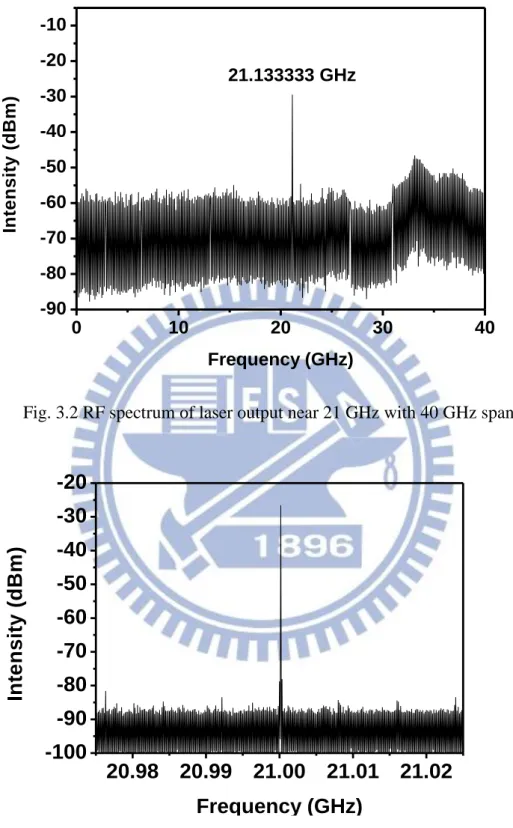
Fig. 3.2 is the RF spectrum to demonstrate the repetition rate can be up to 21 GHz by the rational harmonic mode-locking with p=3 and the side mode suppression ratio performance is well. The Fig. 3.3 shows high mode-locking quality since the supermode suppression ratio (SMSR) is greater than 60 dB.

34 0 10 20 30 40 -90 -80 -70 -60 -50 -40 -30 -20 -10 21.133333 GHz In te n s it y ( d B m ) Frequency (GHz)

Fig. 3.2 RF spectrum of laser output near 21 GHz with 40 GHz span

20.98 20.99 21.00 21.01 21.02 -100 -90 -80 -70 -60 -50 -40 -30 -20 In te n s it y ( d B m ) Frequency (GHz)

Fig. 3.3 RF spectrum of laser output near 21 GHz with 50 MHz span

35

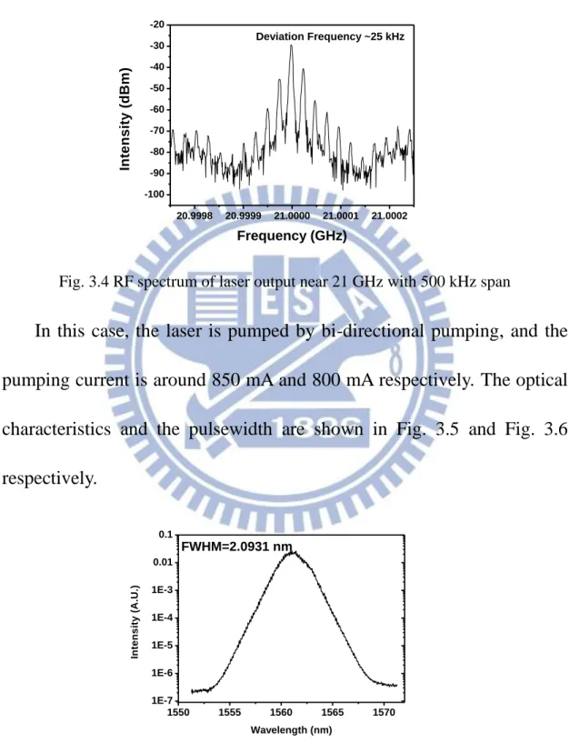
asynchronous mode-locked situation. The deviation frequency in this case is ~25 kHz. 20.9998 20.9999 21.0000 21.0001 21.0002 -100 -90 -80 -70 -60 -50 -40 -30 -20 In te n s it y ( d B m ) Frequency (GHz) Deviation Frequency ~25 kHz

Fig. 3.4 RF spectrum of laser output near 21 GHz with 500 kHz span

In this case, the laser is pumped by bi-directional pumping, and the pumping current is around 850 mA and 800 mA respectively. The optical characteristics and the pulsewidth are shown in Fig. 3.5 and Fig. 3.6 respectively. 1550 1555 1560 1565 1570 1E-7 1E-6 1E-5 1E-4 1E-3 0.01 0.1 In te n s it y ( A .U .) Wavelength (nm) FWHM=2.0931 nm

Fig. 3.5 Optical spectrum of the 21GHz rational asynchronous mode-locked Er-fiber soliton laser

36 75 80 85 90 95 100 105 0.000 0.005 0.010 0.015 0.020 SHG pulse width = 2.6637 (ps)

sech2 pulse width = 1.7297 (ps)

In te n s it y ( A .U .) Time delay (ps)

Fig. 3.6 SHG intensity autocorrelation trace (open circles) and the fitting curve (solid curve) of the laser output, assuming sech2 pulse shape.

Finally, we use the stabilization scheme that is based on controlling the cavity length to lock the deviation frequency at a suitable value [3.1]. Long–term stable mode-locked fiber laser is carried out when the feedback control is turned on. In the 21 GHz rational harmonic mode-locked fiber laser case, the deviation frequency shift can be controlled to be within and the duration of stabilization can be greater than 2000 seconds. The results are shown in Fig.3.7

37

Fig. 3.7 Deviation frequency shift: without the stabilization scheme (red dash line); with the stabilization scheme (black solid line).

Because of the long stable operation duration, we can further measure the laser dynamics in our rational harmonic mode-locked fiber laser system. The results are given in the next section.

38

3.2 Pulse dynamics of ARHM fiber soliton laser

3.2.1 Periodic pulse timing position and center frequency

variation

In the above section, we achieved the high repetition rate by the asynchronous rational harmonic mode-locked method. In this section, we will study the laser dynamics in the ARHM case. We utilize the theory developed in [3.2] to investigate the laser dynamics.

For simplicity we will assume the pulse timing variation is a simple sinusoidal function at the deviation frequency . The detected pulse train signals from the fast photodetector can be expressed as:

(3.1)

where r(t) is the response function of fast photodetector, p(t) is the pulse intensity, is the period of the cavity harmonic, is the half peak-to-peak displacement of sinusoidal pulse timing variation, is the Dirac’s delta function, and is the operation of convolution. The Fourier transform of the photocurrent i(t) can be expressed to be:

(3.2)

39

(3.3) where are the Fourier transforms of the response function of fast photodetector and the pulse intensity respectively, and is the Bessel function of the first kind of order n. As said above, the pulse trains with a sinusoidal timing variation in the time domain can be converted to the frequency domain like a comb as show in Fig. 3.8. From equation (3.3), the sinusoidal timing variation is converted to amplitudes of in the frequency domain, which is spaced equally by the deviation frequency around the harmonic mode ( . Because I(ω ) is proportional to , we can estimate the from the power ratio of the 0th (the cavity harmonic frequency) and 1st (the modulation frequency) spectral peaks. It is written as:

)

) (3.4)

We can use the equation (3.4) to calculate the pulse timing variation for the asynchronous rational harmonic mode-locked fiber lasers.

40

For comparing with the experimental data, we will use the approximate analytic formula derived in [3.2], which is given below:

(3.5)

(3.6)

Also from [3.2], we know the phase difference between the pulse timing variation and the pulse center frequency variation is . The pulse center frequency variation can be identified by comparing the timing variation before and after a propagation length of SMF-28. The formula is shown as below:

(3.7) where the term is the extra pulse timing variation resulted from the dispersion of external SMF-28. Equation (3.7) can be derived to get the equation (3.8)

(3.8) where and are the timing variations after and before SMF-28 respectively.

41

The RF spectra with span 500 kHz are shown in the Fig. 3.8, Fig. 3.9, Fig. 3.10, and Fig. 3.11. The pulse trains propagate through the external section of SMF-28 with the length of 0m, 200m, 300m, and 500m respectively. 20.9997 20.9998 20.9999 21.0000 21.0001 21.0002 21.0003 -100 -90 -80 -70 -60 -50 -40 -30 -20 0m f=26kHz y=14.5dBm X = 21.000027, Y = -38.83 X = 20.999973, Y = -44.83 X = 21.000001, Y = -27.33 In te n s it y ( d B m ) Frequency (GHz)

Fig. 3.8 RF spectrum at 21 GHz with 0 m SMF 28 fiber

20.9997 20.9998 20.9999 21.0000 21.0001 21.0002 21.0003 -100 -90 -80 -70 -60 -50 -40 -30 X = 21.00001, Y = -43 X = 20.999958, Y = -48.16 X = 20.999983, Y = -32.5 P o w e r ( d B m ) Frequency (GHz) L=200m f=27kHz y=13.08dBm

42 20.9997 20.9998 20.9999 21.0000 21.0001 21.0002 21.0003 -100 -90 -80 -70 -60 -50 -40 -30 X = 21.000009, Y = -40.5 X = 20.999957, Y = -46.5 X = 20.999983, Y = -32.16 P o w e r ( d B m ) Frequency (GHz) L=300m f=26kHz y=11.34dBm

Fig. 3.10 RF spectrum near 21 GHz with 300 m SMF 28 fiber

20.9997 20.9998 20.9999 21.0000 21.0001 21.0002 21.0003 -100 -90 -80 -70 -60 -50 -40 -30 X = 21.00001, Y = -39.16 X = 20.999984, Y = -35 X = 20.999957, Y = -46.5 P o w er ( d B m ) Frequency (GHz) L=500m f=27kHz y=7.83dBm

Fig. 3.11 RF spectrum near 21 GHz with 500 m SMF 28 fiber

According to these data and equation (3.4), the relation between the external section of SMF-28 and pulse timing variation is shown in Fig. 3.12

43 0 100 200 300 400 500 3 4 5 6 Di spl ace m en t of t he pu lse t im in g (ps) Length of SMF28 (m)

Fig. 3.12 Measurement of the net pulse timing variation versus the length of the SMF-28 fiber.

Furthermore, we take the periodic pulse timing position variation and the parameter of SMF-28 into the question (3.8) to get the pulse center frequency variation. The experimental and calculated results are listed in Table 3.2.

Table 3.2 Ratios of the RF intensity and the estimated wavelength variation

SMF 28 Length (m) Ia-Ib (dBm) △t (ps) △λ(nm)

0m 14.5 2.80596

200m 13.08 3.28278 0.5011434

300m 11.34 3.96577 0.5495068

44

Finally, the average pulse center frequency variation of △λ is 0.545092 nm. We have measured and saved the RF spectra for different lengths of SMF-28 fiber and calculated the values of the periodic pulse timing position variation. These results provide us to estimate the effective modulation depth in this particular case. We find that the modulation depth in the asynchronous rational harmonic mode-locked fiber laser is mainly contributed by the higher order harmonics from the electronic amplifier.

45

3.2.2 Determination of the effective modulation depth

The journal paper [3.3] indicated that the rational harmonic mode-locking with a phase modulator is mainly due to the contributions of higher order harmonics from the amplified electrical driving signal. In this section, we will use another way to determine the conclusion of [3.1]. Based on the section 3.3.1 results, we can further use these results to calculate the effective modulation depth of the mode-locked fiber laser. In this section, we set two different experimental cases to enhance the accuracy of experiments. The first one is the rational harmonic mode-locking and the other is the harmonic mode-locking. We detune the operation parameters to let their effective modulation strength get close. The equation (3.9) is derived from equation (3.6) and is shown below:

(3.9)

Figure 3.13 is the RF spectrum with no external section of SMF-28 in the rational harmonic mode-locked case. The deviation frequency is ~26 kHz and the power difference of the 0th (the cavity harmonic frequency) and 1st (the modulation frequency) order spectral peaks is 14.5 dB. This

46 is shown in Fig. 3.13. 20.9997 20.9998 20.9999 21.0000 21.0001 21.0002 21.0003 -100 -90 -80 -70 -60 -50 -40 -30 -20 0m f=26kHz y=14.5dBm X = 21.000027, Y = -38.83 X = 20.999973, Y = -44.83 X = 21.000001, Y = -27.33 In te n s it y ( d B m ) Frequency (GHz)

Fig. 3.13 RF spectrum at 21 GHz with 0 m SMF 28 fiber

The second-harmonic generation (SHG) intensity autocorrelation trace is shown in Fig. 3.14 by open circles. With the assumption of sech2 pulse shape, the solid line in Fig 3.14 is the fitting curve of the SHG intensity autocorrelation trace and the pulsewidth is 1.7297 ps.

75 80 85 90 95 100 105 0.000 0.005 0.010 0.015 0.020 SHG pulse width = 2.6637 (ps) sech2 pulse width = 1.7297 (ps)

In te n s it y ( A .U .) Time delay (ps)

47

curve) of the laser output, assuming sech2 pulse shape.

The simulation parameters used here are listed in Table 3.3

Table 3.3 Simulation parameters in rational harmonic mode-locking

The simulation parameters (Rational harmonic mode-locking) 26 kHz 8 MHz 21 GHz 0.05 0.2 1.7297 ps 2.80596 ps

These parameters are normalized by a time units of 0.5 ps, which is near the laser pulsewidth. The value of is determined from the filter bandwidth (13.5 nm) and the value of is determined from the

estimated cavity average dispersion (-4.1ps2/km) as we well as the cavity length (25m). After substituting these parameters in equation (3.9), we get the effective modulation depth (M) to be 0.091917.

The comparative case is the harmonic mode-locking. The RF spectrum and pulsewidth profiles are given in Fig. 3.15 and Fig. 3.16 respectively.

48 20.9997 20.9998 20.9999 21.0000 21.0001 21.0002 21.0003 -110 -100 -90 -80 -70 -60 -50 -40 -30 -20 X = 20.999958, Y = -40.33 X = 21.000042, Y = -37.5 X = 21, Y = -24.5 P o w e r (d B m ) Frequency (GHz) L=0m f=42 kHz y=14.415

Fig. 3.15 RF spectrum at 21 GHz with 0 m SMF 28 fiber

-15 -10 -5 0 5 10 15 20 0.06 0.07 0.08 0.09 0.10 0.11 SHG pulse width = 2.1313 (ps) sech2 pulse width = 1.384 (ps)

In te n si ty ( A .U .) Time delay (ps)

Fig. 3.16 SHG intensity autocorrelation trace (open circles) and the fitting curve (solid curve) of the laser output, assuming sech2 pulse shape.

49

Table 3.4 Simulation parameters in harmonic mode-locking

The simulation parameters (Harmonic mode-locking) 42 kHz 8 MHz 21 GHz 0.05 0.2 1.384 ps 2.8326 ps

After substituting these parameters in equation (3.9), we get the effective modulation depth (M) is 0.241585. And a comparison table is given below.

Table 3.5 Comparison table between harmonic mode-locking and rational harmonic mode-locking Harmonic mode-locking Rational harmonic mode-locking Delta dBm 14.415 dBm 14.5 dBm Timing variation 2.8326 ps 2.80596 ps Deviation frequency 42 kHz 26 kHz Pulsewidth (sech^2 shaping) 1.384 ps 1.7297 ps

Effective modulation depth M: 0.241585 M: 0.091917 Effective modulation power 1.16037 dBm -7.23313 dBm

50

The effective modulation can be related to the driving power of the modulator with the dBm unit. The formula is given below:

M (dBm) = (3.10)

The experimental modulation power injected into the modulator is ~14 dBm in the harmonic mode-locking and >5.34 dBm in the rational harmonic mode-locking respectively. The difference between the experimental values and theoretical ones may be caused by the noise disturbances from the laser system. However, it matches the result that broad pulsewidth with low modulation depth in rational harmonic mode-locking by referring to reports of C. Wu and N. K. Dutta [3.6]. Base on the laser dynamics of asynchronous harmonic mode-locking, we calculate a lower modulation depth in the rational harmonic mode-locking case. This is another way to demonstrate the rational harmonic mode-locking with a phase modulator is mainly due to the contributions of the higher order harmonic terms from the amplified electrical driving signal.

51

3.3 33GHz asynchronous rational harmonic mode-locked

Er-fiber soliton laser

In this section, we improve our laser system to operate at 33 GHz asynchronous rational harmonic mode-locking. In the frequency domain we show the results of RF spectrum in the Fig 3.17, Fig. 3.18 and Fig. 3.19. 0 10 20 30 40 -80 -60 -40 -20 0 P o w e r (d B m ) Frequency (GHz)

Fig. 3.17 RF spectrum of laser output near 33 GHz with 40 GHz span

As shown in Fig. 3.17 we observe certainly that the repetition rate of 33 GHz has been achieved, when the modulation frequency is operated at 11 GHz with p=3 and the sidemode suppression ratio performance is very well. The bandwidth of the RF amplifier we used is 26.5 GHz.

52 32.98 32.99 33.00 33.01 33.02 -80 -70 -60 -50 -40 -30 -20 P o w e r (d B m ) Frequency (GHz)

Fig. 3.18 RF spectrum of laser output near 33 GHz with 50 MHz span

As shown in the Fig. 3.18 the supermode noise suppression is suppressed very well.

33.1120 33.1121 33.1122 33.1123 33.1124 -90 -80 -70 -60 -50 -40 -30 -20 In te n s it y ( d B m ) Wavelength (nm) 34kHz

Fig. 3.19 RF spectrum of laser output near 33 GHz with 500 kHz span

Fig. 3.20 shows the optical spectrum of the laser output. The full-width half-maximum (FWHM) bandwidth of the optical spectrum is 1.28 nm.

53 1545 1550 1555 1560 1565 1E-7 1E-6 1E-5 1E-4 1E-3 0.01 0.1 In te n s it y ( A .U .) Wavelength (nm) FWHM=1.28 nm

Fig. 3.20 Optical spectrum of the 33GHz asynchronous rational mode-locked Er-fiber soliton laser

Finally, the pulse profile is shown in Fig. 3.21 and with the assumption of sech2 pulse shape, indicating that the pulsewidth is 2.5477 (ps). 65 70 75 80 85 90 95 100 0.00 0.01 0.02 0.03 SHG pulse width = 3.9234 (ps) sech2 pulse width = 2.5477 (ps)

In te n si ty ( A .U .) Time delay (ps)

Fig. 3.21 SHG intensity autocorrelation trace (open circles) and the fitting curve (solid curve) of the laser output, assuming sech2 pulse shape.

54

3.4 New synchronous harmonic mode-locked operation

state

When we measured the laser dynamics as mentioned above, we also found a new mode-locked fiber laser operation state. This mode-locked situation exhibits spectral peaks at a larger deviation frequency than the deviation frequency of ARHML in our knowledge. This new state also exhibits high SMSR as shown in Fig. 3.23 and Fig. 3.29. The allowed region of the deviation frequency is very small so that it can provide us an obvious operating point (i.e. the laser gets mode-locked perfectly once it enters this large deviation frequency region). Finally, we can also employ the long-term stabilization scheme based on the deviation-frequency locking to stabilize the laser. We also show that both the harmonic mode-locked case and the rational harmonic mode-locked case can be operated in this new state.

We first demonstrate the harmonic mode-locked fiber laser with a large deviation frequency. The experimental setup is the same as in Fig. 3.1. The results in this case include the RF spectrum, pulsewidth profile, optical spectrum and laser stabilization. The experimental parameters are listed in Table 3.6.

55

Table3.6 Parameters for the new harmonic mode-locked state

Parameters of harmonic mode-locking

980 nm pump L:850 mA ; R:800 mA

Repetition rate 39.997017 GHz

Synthesizer power -7 dBm

Results

Optical center frequency 1559.32 nm Optical spectrum bandwidth 2.0713 nm

Pulsewidth 1.8412 ps Output power 27 mW SMSR >55 dB Deviation frequency 189 kHz 39.9968 39.9969 39.9970 39.9971 39.9972 -100 -90 -80 -70 -60 -50 -40 -30 -20 X = 39.997187, Y = -43 X = 39.996998, Y = -26.33 P o w e r ( d B m ) Frequency (GHz)

56 39.995 39.996 39.997 39.998 39.999 -100 -90 -80 -70 -60 -50 -40 -30 -20 P o w e r ( d B m ) Frequency (GHz) SMSR>55 dB

Fig. 3.23 RF spectrum at 40 GHz with 50 MHz span and SMSR > 55 dB

70 75 80 85 90 95 100 105 110 0.060 0.065 0.070 0.075 0.080 0.085 0.090 0.095 0.100 SHG pulse width = 2.8335 (ps)

sech2 pulse width = 1.8412 (ps)

In te n s it y ( A .U .) Time delay (ps)

Fig. 3.24 SHG intensity autocorrelation trace (open circles) and the fitting curve (solid curve) of the laser output, assuming sech2 pulse shape.

57 1550 1555 1560 1565 1E-7 1E-6 1E-5 1E-4 1E-3 0.01 In te n s it y ( A .U .) Wavelength (nm) FWHM=2.0713 nm

Fig. 3.25 Optical spectrum of the 40GHz harmonic mode-locked Er-fiber soliton laser

0 1000 2000 3000 4000 5000 6000 18000 18500 19000 19500 20000 Time (second) D e v ia ti o n f re q u e n c y ( H z ) =456.8 Hz

Fig. 3.26 The deviation frequency shift with duration time of stabilization

We then demonstrate the rational harmonic mode-locked fiber laser with large deviation frequency. The results in this case include the RF spectrum, pulsewidth profile and optical spectrum. The experimental

58

parameters are listed in table 3.7.

Table3.7 Parameters in new harmonic mode-locked state

Parameters of rational harmonic mode-locking

980 nm pump L:850 mA ; R:800 mA

Modulation frequency 13.308938 GHz

Synthesizer power 3 dBm

Results

Repetition rate 39.928 GHz

Optical center frequency 1559.12 nm Optical spectrum bandwidth 1.638 nm

Pulsewidth 1.9946 ps Output power 27 mW SMSR ~60 dB Deviation frequency 183 kHz 0 10 20 30 40 -80 -70 -60 -50 -40 -30 -20 -10 P o w e r (d B m ) Frequency (GHz)

59

In the RF spectrum with span 40 GHz, one can see that the unwanted harmonic sidemodes are suppressed very well.

39.9258 39.9259 39.9260 39.9261 39.9262 -100 -90 -80 -70 -60 -50 -40 -30 -20 X = 39.926192, Y = -42.16 X = 39.926009, Y = -26.33 P o w e r (d B m ) Frequency (GHz) Span 500 kHz Deviation frequency 183 kHz

Fig. 3.28 RF spectrum at near 40 GHz in with 500 kHz span

39.925 39.926 39.927 39.928 39.929 -100 -90 -80 -70 -60 -50 -40 -30 -20 P o w e r (d B m ) Frequency (GHz) Span 50 MHz RBW 1 kHz SMSR=~60 dB sweep time 130 sec

Fig. 3.29 RF spectrum at near 40 GHz with 50 MHz span and SMSR ≈ 60 dB

In the RF spectrum with span 50 MHz, one can see that the supermode noises are also suppressed very well.

60 70 75 80 85 90 95 100 105 110 0.050 0.055 0.060 0.065 0.070 0.075 0.080 0.085 SHG pulse width = 3.0716 (ps) sech2 pulse width = 1.9946 (ps)

In te n s it y ( A .U .) Time delay (ps)

Fig. 3.30 SHG intensity autocorrelation trace (open circles) and the fitting curve (solid curve) of the laser output, assuming sech2 pulse shape.

1550 1555 1560 1565 1E-7 1E-6 1E-5 1E-4 1E-3 0.01 0.1 1 FWHM=1.638 nm In te n s it y ( A .U .) Wavelength (nm)

Fig. 3.31 Optical spectrum of the 40GHz rational harmonic mode-locked Er-fiber soliton laser

Even though this situation is quite similar to asynchronous mode-locking, the observed optical spectrum exhibits clear mode spacing

61

and this operation mode is reached by setting the modulation frequency very close to the harmonic frequency of cavity. These characteristics indicate that this new mode-locked state should be close to synchronous mode-locking rather than asynchronous mode-locking. So we start to design a series of experiments to check if this state is asynchronous mode-locking or not. These experiments are given below.

First, we measure the oscillation frequency from the low frequency spectrum of the pulse train and the result is shown in Fig. 3.32.

0.0000 0.0001 0.0002 0.0003 0.0004 0.0005 -100 -80 -60 -40 -20 0 P o w e r (d B m ) Frequency (GHz)

Relaxation oscillation frequency=191kHz

large deviation frequency situation

synchronous mode-locking without modulation

Fig. 3.32 Low frequency spectrum of the output pulse train. Large deviation frequency situation (red dash line), synchronous situation (blue dot line) and no

modulation signal situation (black solid line).