針對多視角視訊合成之景深修正演算法

(1)

國

立

交

通

大

學

多媒體工程研究所

碩

士

論

文

針對多視角視訊合成之景深修正演算法

A depth refinement algorithm for multi-view video synthesis

研究生：石新嘉

指導教授：蕭旭峯教授

(2)

針對多視角視訊合成之景深修正演算法

研究生: 石新嘉指導教授: 蕭旭峯

國立交通大學多媒體工程研究所

摘要

隨著近年來顯示科技、影像擷取及壓縮技術的發展，自由視角電視﹝Free Viewpoint TV﹞、自由視角視訊﹝Free Viewpoint Video﹞以及立體視訊﹝Stereoscopic Video﹞等多視角視訊的應用紛紛發表且受到關注。以上應用為了達到能夠自由變換視角的功能，除了原本的視訊資料之外必須加上景深的資訊。雖然已經有眾多演算法可以預估景深，但是對於預估正確的景深仍有許多挑戰。在這篇論文中，我們使用立體的攝影機設置進行景深估計以節省景深預估所使用的資源並且提出一個景深修正演算法針對景深錯誤的像素進行修正。我們提出的方法先將景深圖中的像素區分為可信的﹝reliable﹞及不可信的﹝unreliable﹞，再針對不可信的像素進行景深修正以得到品質更好的景深圖。除了景深修正演算法，我們也提出一個可信度加權視角合成演算法。最後，我們會以合成視角的品質評估修正過後的景深圖，並且會以主觀的及客觀的實驗結果進行比較。

(3)

A depth refinement algorithm for multi-view video synthesis

Student: Hsin-Chia Shih Advisor: Hsu-Feng Hsiao

Institute of Multimedia Engineering National Chiao Tung University

Abstract

With the recent progress of display, capture device, and coding technologies, multi-view video applications such as free viewpoint TV (FTV), free viewpoint video (FVV), and stereoscopic video have been introduced to the public with growing interest. To achieve free navigation of such applications, depth information is required along with the video data. There have been many research activities in the area of depth estimation; however it still poses us great challenge to estimate accurate depth map. In this paper, we use stereo camera setting to estimate depth map in order to save the resources to be used in depth estimation and propose a depth refinement algorithm for recovering bad depth pixels. The proposed algorithm classifies the pixel-wise depth map into two categories, one is reliable and the other is unreliable, followed by the depth refinement algorithm for those pixels with unreliable depth values. Except for the depth refinement algorithm, we also propose a reliable weighted view interpolation algorithm. At last, the refined depth map is evaluated by the quality of the synthesized views subjectively and objectively.

(4)

Acknowledgement

能夠完成這篇論文，首先必須要感謝老師的指導。在無數次的挫折中，老師總是循序漸進地帶領我慢慢找出問題的癥結，提醒應該要注意的方向。老師也教導了我許多求學上的正確態度，讓我獲益良多，最後終於完成這篇論文。同時也要感謝實驗室的伙伴們，不僅讓我在研究上有共同討論的對象，你們在我研究和生活遇到瓶頸的時候，也能適時地給予支持。最後，謹將這篇論文獻給我最摯愛的父母以及家人。

(5)

-List of Tables

Table 11: Applications of FTV [1] ... 1

Table 41: Test sequences and virtual views to be synthesized ... 35

Table 42: PSNR and PSPNR results of virtual view 8 of sequence BookArrival (30 pixels excluded)... 46

Table 43: PSNR and PSPNR results of virtual view 8 of sequence BookArrival (No pixel excluded)... 48

Table 44: PSNR and PSPNR results of virtual view 6 of sequence Lovebird1 (30 pixels excluded). ... 49

Table 45: PSNR and PSPNR results of virtual view 6 of sequence Lovebird1 (No pixel excluded). ... 51

Table 46: PSNR and PSPNR results of virtual view 5 of sequence Newspaper (30 pixels excluded). ... 53

Table 47: PSNR and PSPNR results of virtual view 5 of sequence Newspaper (No pixel excluded). ... 55

(8)

-List of Figures

Figure 11: Videoplusdepth data representation... 3

Figure 12: Example of an FTV system and data format [1]. ... 3

Figure 21: Relation between disparity and depth [14]. ... 7

Figure 22: Configuration of view synthesis [21]. ... 10

Figure 23: Block diagram of the view synthesis for VSRS [3]. ... 11

Figure 31: Configuration of depth estimation... 16

Figure 32: Reference view selection from two camera baseline distance away... 16

Figure 33: Stereo camera setting for depth estimation. ... 17

Figure 34: Flow chart of the proposed algorithms. ... 19

Figure 35: Results of depth estimation (BookArrival). ... 20

Figure 36: Crosschecking procedure... 21

Figure 37: Results of depth consistency check... 22

Figure 38: Similar texture areas. ... 23

Figure 39: The occluded area in the left image can not be seen in the right image... 24

Figure 310: The results of occlusion detection. ... 25

Figure 311: Consideration of reliability... 26

Figure 312: Relation of unreliable depth pixel and fourneighbor reliable depth pixels. ... 27

Figure 313: Depth value filtering. ... 29

Figure 314: Refinement of uncovered area. ... 30

Figure 315: Results of sequence BookArrival after applying depth refinement algorithm. ... 31

Figure 316: Results of sequence Lovebird1 after applying depth refinement algorithm... 32

Figure 317: Results of sequence Newspaper after applying depth refinement algorithm... 32

Figure 41: Experimental results of frame #58 of sequence BookArrival. ... 37

Figure 42: Enlarged results from figure 41... 38

Figure 43: Experimental results of frame #73 of sequence BookArrival. ... 38

Figure 45: Experimental results of frame #6 of sequence Lovebird1... 40

Figure 47: Experimental results of frame #35 of sequence Lovebird1... 42

Figure 49: Experimental results of frame #0 of sequence Newspaper. ... 44

Figure 411: Frame PSNR of virtual view 8 of sequence BookArrival (30 pixels excluded)... 46

(9)

Figure 413: Frame T_PSPNR of virtual view 8 of sequence BookArrival (30 pixels excluded)... 47

Figure 414: Frame PSNR of virtual view 8 of sequence BookArrival (No pixel excluded). ... 48

Figure 415: Frame S_PSPNR of virtual view 8 of sequence BookArrival (No pixel excluded)... 48

Figure 416: Frame T_PSPNR of virtual view 8 of sequence BookArrival (No pixel excluded)... 49

Figure 417: Frame PSNR of virtual view 6 of sequence Lovebird1 (30 pixels excluded)... 50

Figure 418: Frame S_PSPNR of virtual view 6 of sequence Lovebird1 (30 pixels excluded). ... 50

Figure 419: Frame T_PSPNR of virtual view 6 of sequence Lovebird1 (30 pixels excluded). ... 51

Figure 420: Frame PSNR of virtual view 6 of sequence Lovebird1 (No pixel excluded)... 52

Figure 421: Frame S_PSPNR of virtual view 6 of sequence Lovebird1 (No pixel excluded). ... 52

Figure 422: Frame T_PSPNR of virtual view 6 of sequence Lovebird1 (No pixel excluded). ... 53

Figure 423: Frame PSNR of virtual view 5 of sequence Newspaper (30 pixels excluded). ... 54

Figure 424: Frame S_PSPNR of virtual view 5 of sequence Newspaper (30 pixels excluded)... 54

Figure 425: Frame T_PSPNR of virtual view 5 of sequence Newspaper (30 pixels excluded)... 55

Figure 426: Frame PSNR of virtual view 5 of sequence Newspaper (No pixel excluded). ... 56

Figure 427: Frame S_PSPNR of virtual view 5 of sequence Newspaper (No pixel excluded)... 56

(10)

-Chapter 1. Introduction

In recent years, since various multimedia services have become available and the researches in the areas of three-dimensional (3D) displays, digital video broadcast and computer vision algorithms have enormous progress, the demands for realistic multimedia systems are growing rapidly. A number of 3D video technologies have been studied to satisfy these demands. Among the related 3D video technologies, multi-view video is the key technology for various applications, including free-viewpoint video (FVV), free-viewpoint television (FTV), immersive teleconference, and 3DTV.

The traditional video is a two-dimensional (2D) medium and only provides a passive way for viewers to observe the scene. However, FTV significantly extend the sensation of classical 2D video, it is an innovative visual media that enables viewers to view a 3D scene by freely changing their viewpoints as if they were there or/and provides a 3D depth impression of a virtual scene. In such scenario, the viewers can experience the free viewpoint navigation within the range covered by the shooting cameras. The ability of free navigation can be used in a very wide range of application domain as shown in Table 1-1 [1].

Table 1-1: Applications of FTV [1]

Field Examples

Entertainment

TV/Broadcast

Fixed media (eg. optical discs, solid state) Personal cam-cording

Informational realistic visual quality game

(11)

and Expo

immersive photo album

advertisement interactive and realistic presentation

nature observation realistic bird watching, safari, undersea park sightseeing immersive virtual sightseeing

museum interactive and realistic exhibition

art/content creation of new media art and digital content video production interactive camera motions video production archive multi-angle archive, living national treasures,

traditional entertainment education interactive remote education

medicine realistic virtual examination, operation, education security, surveillance realistic audio-visual surveillance for store, factory,

building, street, public facilities transportation traffic monitoring at intersection, ITS

To achieve free navigation functionality, depth information is required in addition to video signals. The data representation, which is often called video-plus-video is shown in Figure 1-1. Figure 1-2 [1] shows an example of an FTV system that transmits multi-view video with depth information. The content may be produced in a number of ways, e.g., with multi-camera setup, depth cameras or 2D/3D conversion processes. At the receiver, depth-image-based rendering could be performed to project the signal to various types of displays.

(12)

Figure 1-1: Video-plus-depth data representation.

Figure 1-2: Example of an FTV system and data format [1].

Based on this configuration, the virtual view of arbitrary view angle can be synthesized by color video data and depth maps providing a Z-value for each pixel. The visual quality of the synthesized virtual view is highly related to the precision of the depth map. Depth map can be generated by depth camera, however, such devices are not often seen and there are certain restrictions for the devices to acquire the depth map at high resolution. Alternatively, the depth map can be estimated by two or more videos captured at different angles conventionally. There have been many researches of depth estimation; however there is still room to improve the accuracy of depth map. There might be unreliable depth values around

(13)

the occluded area in the estimated depth map. These unreliable depth values are the main cause of bad visual quality of the synthesized virtual views.

In order to raise the visual quality of synthesized virtual view, we propose a depth refinement algorithm to correct the unreliable depth value in depth map before view synthesis is carried out and a reliable/unreliable weighting interpolation function is proposed to be included in the view synthesis algorithm [3] to further improve the visual quality of synthesized virtual views.

The rest of this paper is organized as follows. In Chapter 2 we introduce the related works of depth estimation and view synthesis. In Chapter 3 we describe our proposed depth refinement algorithm, followed by Chapter 4, the simulation results and discussions. The concluding remarks are presented in Chapter 5.

(14)

Chapter 2. Related Work

FTV was proposed to MPEG in 2002. There have been a lot of input documents for establishing standardization of FTV since then, including depth estimation and view synthesis algorithms. In this study, our focus is refining the estimated depth map to provide more precise depth map for virtual view synthesis. In the following chapter we will introduce the previous researches about depth estimation, including the method and tools that we adopt. The previous researches about virtual view synthesis for multi-view video will be described in this chapter also.

2.1 Depth Estimation

2.1.1 Stereo matching

For the last two decades, stereo matching has been a well-known 3D depth sensing method [4]. Stereo matching is one of the most active research areas in computer vision and it serves as an important step in many applications (e.g., view synthesis, image based rendering, etc). The goal of stereo matching is to determine the disparity map between an image pair taken from the same scene. Disparity describes the difference in location of the corresponding pixels. However, occlusion area is a major challenge for the accurate computation of visual correspondence. Occluded pixels are only visible in one image, so there is no corresponding pixel in the other image.

(15)

V. Kolmogorov et al. [5] presented a method which properly addresses occlusions, while preserving the advantages of graph cut algorithm. Graph cut algorithm is used to solve the energy minimization problem in computer vision [6] [7]. J.Sun et al. [8] proposed another method which uses a symmetric stereo model to handle occlusion in dense two-frame stereo. It embeds the visibility constraint within an energy minimization framework, resulting in a symmetric stereo model that treats left and right images equally. An iterative optimization algorithm is used to approximate the minimum of the energy using belief propagation [9].

The occlusion problem can be alleviated by using multi-view images. There are several algorithms using multi-view images as input to deal with the occlusion problem and obtain more accurate depth map. Some of these depth estimation algorithms are described in the following sub-sections.

2.1.2 Segment-based depth estimation

S. Lee et al. [10] proposed a method of depth map generation for multi-view video in 2008. This method is a segment-based approach and uses the 3D warping technique. It assumes that the pixels in one segment shall have the same depth value. It employs “Mean Shift based Image Segmentation” scheme in [11] to segment images. After image segmentation, depth estimation is conducted to each segment. To generate the depth image for the center view, both left and right views are considered simultaneously. Since the conventional matching function MSE and MAD are not robust to illumination/color change between cameras, they use self-adaptation dissimilarity measure as a matching function [12]. This function adds the absolute gradient difference term to the existing MAD term and uses a weighting factor between MAD and MGRAD (mean gradient absolute difference). This segment-based depth estimation method was added a refinement step using segment-based

(16)

belief propagation to remove erroneous depth values [13].

2.1.3 Pixel-based depth estimation

M. Tanimoto et al. [14] proposed the pixel-based depth estimation method for FTV. The disparities are estimated first and then they are transformed to depth. This is the method that we utilize to generate initial per-pixel depth map.

The depth estimation method assumes that images captured from each camera are rectified and the cameras are lined up at regular separations in horizontal direction. This method estimates disparities first then it transforms the disparities to depth with the relationship between depth and disparity. Figure 2-1 shows the relation between disparity and depth.

Figure 2-1: Relation between disparity and depth [14].

From this figure, we can easily describe the relation between depth Z, camera interval I, focal length f, and disparity d by the following equation:

(17)

d f I

Z = ⋅ (1)

Because the camera parameters are given, the value of I and f are already known. Once the disparity d is obtained, the depth Z can be derived from equation (1).

The disparity for each pixel is estimated by using stereo matching. It calculates the matching score for each pixel in center view and each disparity value in a predefined range at first. The matching score for a pixel in the center view at disparity d is derived by comparing the intensity value of the pixel (x, y) in the center view against the pixel (x+d, y) in the left view and the pixel (x-d, y) in the right view. Then graph cut algorithm is used to find the appropriate disparities in a view.

After disparity estimation, the depth is derived from disparity and is stored as 8-bit graylevel value with the graylevel 0 representing the furthest depth and the graylevel 255 specifying the nearest depth. The depth value Z of pixel (x, y) is transformed into the 8-bit grayvalue v using the formula described in [15].

This depth estimation algorithm has been implemented in the reference software of depth estimation that has been introduced in MPEG meeting [16].

2.1.4 Temporal consistency for depth estimation

Since the depth estimation method estimates the depth value frame by frame, the result of depth has a low temporal consistency. The depth value of non-moving background often changes frame by frame. Some algorithms are proposed to improve the temporal consistency of depth map.

S. Lee et al. [17] proposed a depth estimation method to enhance the temporal consistency by using a temporally weighted matching function to consider the previous depth value. The whole procedure is the same as their previous research [10] except for the

(18)

matching function. The matching function refers to the depth value of the previous frame when estimating the depth of the current frame. They add a new term C_temp(x,y,d) to the

previous matching function. C_temp(x,y,d) is defined by

| ) , ( | ) , , (x y d d D x y C_temp =λ − _prev (2)

where λ represents the slope of the weighting function and Dprev(x, y) represents the depth

value of the pixel (x, y) in previous frame.

H. Yuan et al. [18] also proposed a depth estimation algorithm that considers mean absolute gradient to enhance depth accuracy in depth discontinuous area. Except adding gradient term in matching function, they based on [17] to propose their depth temporal consistency preserving algorithm. They use a motion mask to decide whether the

) , , (x y d

C_temp term should be added in the matching function or not. The motion mask can be derived by calculating MSE of a pixel. If a pixel is not determined as a motion pixel, the

) , , (x y d

C_temp term will be zero.

G. Bang et al. [19] proposed a depth estimation scheme that assumes the depth value of the non-moving background doesn’t change frame by frame. It extracts non-moving background by calculating frame difference value between current frame and previous frame. When the calculated value is larger than some threshold, the pixel is considered as moving pixel. The mean value of the entire frame difference is used as a threshold. For the fast detection of non-moving background, a frame is divided into blocks. Each block evaluates the cost of the non-moving background block using the derived threshold thn. When the number

of moving pixel is below 10% of the whole pixels in a block, the block is considered as a non-moving block. After dividing frame into non-moving background and moving foreground, graph cut algorithm is used on these results respectively.

(19)

2.2 View Synthesis

As mentioned previously, free navigation functionality can be achieved by synthesizing arbitrary viewpoint video when color video data and per-pixel depth data are obtained. View synthesis is one of the important parts in FTV. The following section is the related work about view synthesis, including the view synthesis algorithm that we used to evaluate our depth refinement algorithm. Since we use the stereo camera setting to estimate depth map, the researches which consider occluded regions will also be introduced in this section.

2.2.1 View synthesis algorithm

View Synthesis Reference Software (VSRS) [3] is the reference software we used to synthesize virtual views. The view synthesis algorithm in VSRS maps the color image data and depth map of reference viewpoint into the target viewpoint by using pixel mapping based on 3D warping [20] or horizontal pixel shift. Here, the reference viewpoint means either the left view or the right view and the target viewpoint means the arbitrary viewpoint between the left view and the right view. The configuration of view synthesis is as follows [21]:

Figure 2-2: Configuration of view synthesis [21].

(20)

The block diagram of this algorithm is shown in Figure 2-3 [3]:

Figure 2-3: Block diagram of the view synthesis for VSRS [3].

In the view synthesis algorithm, the depth map of reference viewpoint is mapped into the target viewpoint at first. The mapped depth map has hole area that has no information from reference view. The small holes in the mapped depth map are filled by median filter. Then, the color data is mapped into target viewpoint by using the filtered depth map. These steps are applied to both left view and right view, there are two color images of target viewpoint are obtained. Large holes in the mapped color image are filled by referring the other mapped color image each other. After hole filling, two different mapped color images are blended according to the ratio of left and right baseline distances. Inpainting is applied to the blended

(21)

image in the final step.

Since the view synthesis algorithm employs 3D warping technique to generate virtual views, the accuracy of depth map directly affects the quality of synthesized view. The depth estimation result is still unstable around boundary and creates boundary noise. It is because of the inaccurate depth value around the object boundary region. C. Lee and Y. S. Ho [22] present a method of boundary filtering. The noise area is located near the boundary of objects having hole. After detecting the hole area, the boundaries of background region are chosen. Then replace the texture information of noise area with the alternative texture information at the other reference view.

2.2.2 Improving view synthesis for multi-view video

There have been a lot of researches on depth estimation for multi-view video, but the quality of the estimated depth map is still not good enough and the pixels with incorrect depth value will cause some artifacts on the synthesized virtual views. J. Sung et al. [23] proposed a method to detect the pixels with bad depth values, then find a better depth value for the pixels, and replace the bad depth value with the better one.

The detection of pixels with bad depth is performed in the merging process of the view synthesis reference software [3]. This detection algorithm is applied to the pixels that are visible in the left and right view images simultaneously. The pixels that have bad depth value in the virtual view image are detected by examining the difference between the two color values and the difference between the two depth values.

The detected bad pixels are grouped by applying connected component analysis. Then the proposed depth correction algorithm finds a depth offset value for a group of bad pixels. If the depth value of the warped depth map is correct, the points that are mapped into left view

(22)

and right view must be the same. The difference between left mapped point and right mapped point is taken as the depth quality measure metric. The depth value which has smaller difference is assumed to be good. The depth correction algorithm is based on this assumption. The depth offset doff will be added to the depth value d and the difference with new depth d’ = d+doff is calculated. The depth offset value is searched twice, one is searched for the depth

value of the warped left depth map LD’ and the other is searched for the depth value of the warped right depth map RD’. The d’ which has smaller difference will be the new depth value for the bad depth pixel.

2.2.3 View synthesis for stereo vision

In the earlier researches of stereo vision, the presence of depth discontinuities and occluded regions are the most notorious problems. There have been some algorithms proposed to handle the occluded regions. D. Scharstein [24] proposed a method to deal with partially occluded regions that are visible from only one camera and have unknown depth. This method assigns explicit depth to the points in occluded regions. The detection of occluded regions is to separately compute the two disparity maps d12 and d21, which are

required by the view synthesis algorithm, and then to label those points as occluded whose disparities disagree. The depth assignment has to rely on heuristics, as there are an infinite number of possible depth interpretations. However, there are a number of choices: (a) interpolating the depth values between the points of known depth, (b) assuming constant depth, or (c) assuming constant depth gradient. Assuming constant depth (b) is easiest and most stable, and has also produced good results in the experiments.

J. S. McVeigh et al. [25] also proposed a method to handle occluded regions. They handle the synthesis from occluded regions by making best reasonable assumptions of the

(23)

scene. These assumptions are that occluded regions have constant depth, and that this depth is equal to the depth of the unoccluded region located on the appropriate side of the occlusion. If the occlusion is visible in the left image, the appropriate side is to the left of the occlusion, and vice versa for an occlusion in the right image. These assumptions, when valid, allow for depth information to be inferred for occluded regions, resulting in accurate intermediate view synthesis for these regions.

(24)

Chapter 3. Proposed Depth Refinement

Algorithm

As mentioned in [23], the quality of estimated depth map is not perfect and bad depth value will be a big impact to visual quality of synthesized virtual views. We propose an algorithm to refine the incorrect depth value to provide a more precise depth map for multi-view video synthesis.

In this chapter, we will describe our proposed depth refinement algorithm in detail. The depth estimation methods mentioned in last chapter use the same camera setting which is used in [21]. The configuration of depth estimation we use is not the same, and the different setting will be described in section 3.1. The detail of our algorithm will be presented in the following section. Except for the depth refinement algorithm, we also make a change in the view synthesis process. The modified part of view synthesis will be described in the last section.

3.1 Camera Setting for Depth Estimation

3.1.1 Camera setting in related works

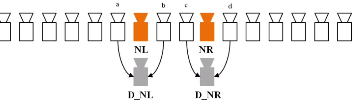
The camera setting for depth estimation methods [10] [14] [15] [17] [18] [19] is shown in Figure 3-1. NL and NR are the views need depth map. D_NL and D_NR are the estimated depth maps for view NL and view NR. Configuration in Figure 3-1 selects neighboring two

(25)

views of NL and NR as reference views (e.g. a, b are the reference views for NL; c, d are the reference views for NR). There is no rule of selecting reference views in depth estimation process, the reference views can also be selected from two baseline distance ahead and two baseline distance behind. This configuration is illustrated as Figure 3-2.

Figure 3-1: Configuration of depth estimation.

Figure 3-2: Reference view selection from two camera baseline distance away.

In this camera setting, we need at least four cameras to estimate the depth map D_NL and D_NR, just like Figure 3-2 illustrated. NL is the left reference view of NR and NR is the right reference view of NL. If a view is at the left or right-most, this camera setting can not be applied because the view at the left-most doesn’t have left reference view and the view at the right-most doesn’t have the right reference view.

D_NL NL

D_NR

(26)

3.1.2 Stereo camera setting

In order to avoid the edge-view problem of the depth estimation algorithms with the camera setting in [21] where either the left-most or the right-most view has only one side of reference view, we don’t use the same camera setting. We use the stereo camera setting which means the view needed to estimate its depth map only uses the view at its left side or at its right side as the reference view. This camera setting not only avoids the edge-view problem but also decreases the number of reference views available for the depth estimation. The stereo camera setting is shown in Figure 3-3.

Figure 3-3: Stereo camera setting for depth estimation.

Since we change the camera setting in depth estimation, the error function used in [14] needs to be modified. The error function is modified as follows:

If the reference view is at left side, the error function is:

) , , ( ) , , (x y d E x y d E = _L (3)

Otherwise, if the reference view is at right side:

) , , ( ) , , (x y d E x y d E = _R (4)

where E(x,y,d) is the error function, EL(x,y,d) is the difference of intensity value between the

D_NL NL

D_NR NR

(27)

current view and left view, and ER(x,y,d) is the difference of intensity value between the

current view and right view.

3.2 Depth Refinement Algorithm

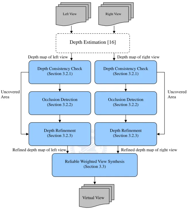
In this section, the proposed algorithm will be described in detail. The flow chart of the whole depth refinement process and also the reliable weighted view synthesis algorithm is shown in Figure 3-4. The result of depth estimation using stereo camera setting is shown in figure 3-5. The right view is the view 7 of the sequence “BookArrival” provided by HHI [26] and the left view is the view 10 of that sequence. The right view and the left view mentioned in this section represent the same viewpoint of the sequence “BookArrival”. The depth value consistency of the two estimated depth map is checked first. Each pixel of the depth map will be classified into two categories, one is reliable depth value pixel and the other is unreliable depth value pixel. Then unreliable pixels are classified into covered and uncovered unreliable depth value pixel. The covered unreliable depth value pixels will go through occlusion detection to divide the unreliable area into occluded area and non-occluded area. The final step is to refine these unreliable depth value pixels. The detail description of each step in the depth refinement process is given below.

(28)

Figure 3-4: Flow chart of the proposed algorithms.

Uncovered Area

Depth map of right view Depth map of left view

Left View

Occlusion Detection (Section 3.2.2)

Right View

Depth Consistency Check (Section 3.2.1)

Depth Refinement (Section 3.2.3)

Depth Estimation [16]

Refined depth map of right view Uncovered Area

Reliable Weighted View Synthesis (Section 3.3)

Occlusion Detection (Section 3.2.2) Depth Consistency Check

(Section 3.2.1)

Depth Refinement (Section 3.2.3)

Virtual View Refined depth map of left view

(29)

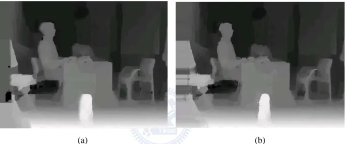
(a) (b) Figure 3-5: Results of depth estimation (BookArrival).

(a) Depth map of the left view, (b) Depth map of the right view

3.2.1 Depth consistency check

Most of the depth values of the estimated depth map are reliable which means the depth values can be used in view synthesis process to find the correct pixel values in reference views. Since the depth estimation method is to find the depth value that can minimize the intensity difference, the depth value of some areas might be estimated incorrectly. These areas include occluded area and uncovered area which are visible in one view but invisible in the other view. These incorrectly estimated depth values are specified as unreliable depth values. Only the unreliable depth values are needed for refinement, so we classify each depth map to two categories first.

In this step, cross-checking is used to check whether the depth value of a pixel is reliable or unreliable. Cross-checking for the left view computes the matchness of the pixel position from the left view to the right view and then from the right view back to the left view based on the corresponding depth map before refinement. A pixel is marked as unreliable if it maps to a pixel that does not map back to it. The cross-checking for the right view is similar.

(30)

Cross-checking is illustrated as Figure 3-6, d(x,y) is the depth value of pixel (x,y) and d(x’,y’) is the depth value of corresponding pixel (x’,y’).

Figure 3-6: Cross-checking procedure.

If the depth value of a pixel (x,y) is correct we can use the depth value of this pixel to find the corresponding pixel (x’,y’) in the other view and use the depth value of the corresponding pixel to map back. The remapped pixel (x”,y”) should be exactly the same as pixel (x,y), theoretically. However, there exists some calculation error when rounding off pixel position to the nearest integer pixel. Thus, we tolerate some error when performing cross-checking. The results of the depth consistency check are shown in Figure 3-7. The pixels classified into unreliable are marked as white and the pixels classified into reliable are marked as black. The pixels marked as gray color are the pixels that can not find the corresponding pixels in the other view, and those pixels are mapped to the position outside the other view. These gray pixels are defined as “uncovered depth pixels” that are also unreliable pixels since these pixels can not be remapped correctly.

Using d(x,y) to map to (x’,y’)

(31)

(a) (b) Figure 3-7: Results of depth consistency check.

(a) Depth consistency map of the left view, (b) Depth consistency map of the right view

3.2.2 Occlusion detection

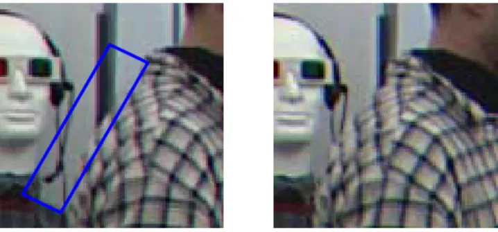
From the results of depth consistency map, we can see that the unreliable areas include not only occluded areas but also uncovered areas. By comparing the depth consistency map and the original video data, some areas that have the similar texture are also classified into unreliable. The areas marked by red lines in Figure 3-8 are examples of those areas with similar texture.

(32)

(a) (b) Figure 3-8: Similar texture areas.

(a) Original video data, (b) Depth consistency map

The refinement method for these similar texture areas is not the same as the method for the occluded areas. Thus, the unreliable pixels need to be classified into occluded pixels and non-occluded pixels further.

Since the matching function used in depth estimation is finding a depth value that minimizes the intensity difference between the current pixel and the corresponding pixel. And the occluded pixels are visible in one view but invisible in the other view. We assume that if a pixel is occluded as illustrated in Figure 3-9, its depth value must be unreliable. If this depth value is used to find the corresponding pixel in the other view, there is a good chance that the depth value of the corresponding pixel is reliable. Based on this assumption and observation, the occlusion detection determines a pixel to be in the occluded area if this pixel is unreliable from the results of the depth consistency check and its corresponding pixel mapped by the unreliable depth should be viewable in the other view and thus should be reliable according to the cross-checking of the depth consistency.

(33)

Figure 3-9: The occluded area in the left image can not be seen in the right image.

The occlusion detection can be expressed as follows:

The following is the results of occlusion detection where white pixels are the occluded area. The depth consistency map can remove these pixels and the rest of inconsistent pixels belong to the non-occluded unreliable area.

for each pixel (x,y) of the depth consistency map {

if(DC(x,y) == unreliable) {

find the corresponding pixel (x’,y’) in the depth consistency map of the other view using the depth value d(x,y)

if(DC’(x’,y’) == reliable)

marks this pixel (x,y) as occluded pixel else

marks this pixel (x,y) as non-occluded pixel }

}

DC(.): value of the depth consistency map of the current view DC’(.): value of the depth consistency map of the other view

(34)

(a) (b) Figure 3-10: The results of occlusion detection.

(a) Occluded area of the left view, (b) Occluded area of the right view

3.2.3 Depth refinement

After the previous steps, the unreliable depth value pixels are divided into three categories. The refinement methods for different categories are similar. They are based on the same idea, but there is a little bit difference between the refinement methods for each category. The detail description of the refinement method is given below.

The main idea for the refinement step is finding the closest reliable depth value pixels and using the depth value of these pixels to interpolate the depth value for the unreliable pixel. Four-neighbor interpolation of the depth value is proposed here, which means the depth value of the unreliable depth pixel is interpolated from the depth values of its top, bottom, left, and right-nearest reliable depth pixels. If the unreliable depth pixel can not find reliable depth pixel in one direction, the weighting factor for this direction is zero and the interpolated depth value is calculated from the other directions.

Conventionally, the weighting factor for each direction is inversely proportional to the distance from the unreliable depth pixel to the reliable depth pixel when applying

(35)

interpolation function. We not only consider the inverse proportion of distance but also consider the reliability of the found reliable depth pixel. The reason is when we use the depth value of the reliable depth pixel to find the corresponding pixel in the other view, the depth value of the corresponding pixel may not be reliable. If the found nearest reliable depth pixel has such property, the reliability of this pixel should be lower than that of the pixel which has reliable corresponding pixel. Thus, we propose a reliable weighted interpolation function. The consideration of reliability can be illustrated as Figure 3-11.

Figure 3-11: Consideration of reliability.

In Figure 3-11, “a” and “c” indicate the reliable depth pixels that map to the unreliable depth pixels in the other view; “b” and “d” indicate the reliable depth pixels that map to the reliable pixels. Thus, reliability of top and left reliable depth pixels should be lower than right and bottom reliable depth pixels.

Let WDTop, WDBottom, WDLeft, and WDRight be the weighting factors calculated by the

distance from current unreliable depth pixel to the nearest reliable depth pixel in each direction. The derivation of these distance weighting factors is described as follows.

a

b

c

d

: Unreliable Area

: Reliable Area

(36)

Figure 3-12: Relation of unreliable depth pixel and four-neighbor reliable depth pixels.

In Figure 3-12, dtop, dbottom, dleft, and dright are the distance to the four closest reliable

pixels. The weighting factors for each direction is

Right Left Bottom Top Top Top Quo Quo Quo Quo Quo WD + + + = Right Left Bottom Top Bottom Bottom Quo Quo Quo Quo Quo WD + + + = Right Left Bottom Top Left Left Quo Quo Quo Quo Quo WD + + + = Right Left Bottom Top Right Right Quo Quo Quo Quo Quo WD + + + = (5)

where QuoDirection is represented as

Direction right left bottom top Direction d d d d d Quo = ⋅ ⋅ ⋅ (6)

where “Direction” in lower index can be either Top, Bottom, Left, or Right.

WHighR and WLowR are the weighting values of high reliability reliable depth pixel and low

reliability reliable depth pixel, respectively. The calculation of proposed weighting factor for each direction is described as follows:

dleft

dright dtop

dbottom

_{: Unreliable Area}

: Reliable Area

(37)

if the reliable depth pixel is found to have high reliability HighR Direction Direction WD W WD '= ⋅ ₍₇₎ else LowR Direction Direction WD W WD '= ⋅ (8)

where “Direction” in lower index can be either Top, Bottom, Left, or Right.

Since the weighting factor for each direction is multiplied by WHighR or WLowR, the

summation of four weighting factors is not equal to 1. The weighting factor for each direction should be rescaled so that their summation equals 1. The final weighting factors are shown below: ' ' ' ' ' " Right Left Bottom Top Top Top WD WD WD WD WD WD + + + = ' ' ' ' ' " Right Left Bottom Top Bottom Bottom WD WD WD WD WD WD + + + = ' ' ' ' ' " Right Left Bottom Top Left Left WD WD WD WD WD WD + + + = ' ' ' ' ' " Right Left Bottom Top Right Right WD WD WD WD WD WD + + + = (9)

The depth value of unreliable depth pixel is interpolated by the following equation: "

" "

" _Bottom _Bottom _Left _Left _Right _Right

Top Top

Unreliable D WD D WD D WD D WD

D = ⋅ + ⋅ + ⋅ + ⋅ (10)

Here, DUnreliable, DTop, DBottom, DLeft, and DRight are the depth values of unreliable depth

pixel, top reliable depth pixel, bottom reliable depth pixel, left reliable depth pixel, and right reliable depth pixel, respectively.

The calculation of the interpolation weighting factors described above serves as the basis of the proposed depth refinement algorithm with some modification for each of the uncovered area and occluded area, respectively. The difference of each category is listed as following:

(38)

The calculation of weighting factor and depth value interpolation can be used directly in non-occluded area.

2. Occluded area

If a pixel is determined as an occluded pixel, its four-neighbor reliable depth pixels are still searched first. Then the reliable depth pixels used to interpolate depth value of occluded pixel are selected as the following.

The depth value is represented from 0 to 255, the smaller depth value means the pixel is in the deeper depth plane. Thus, the object which has smaller depth value will be occluded by the object which has larger depth value. The smallest depth value of the four-neighbor reliable depth pixels is chosen as a reference to filter out the neighbor in the foreground. The difference between this reference depth value and the depth value of reliable depth pixel in the other directions is then calculated. If the difference of any direction is larger than a threshold, the reliable depth pixel in this direction is considered as foreground and discarded. The depth value filtering process is illustrated in Figure 3-13. With depth value filtering we can remove the depth value of the foreground object.

Figure 3-13: Depth value filtering.

After depth value filtering, the depth value of the occluded pixel is interpolated using the same process as non-occluded area.

3. Uncovered area Re Re Re Re Occ Re: Reliable Occ: Occluded

(39)

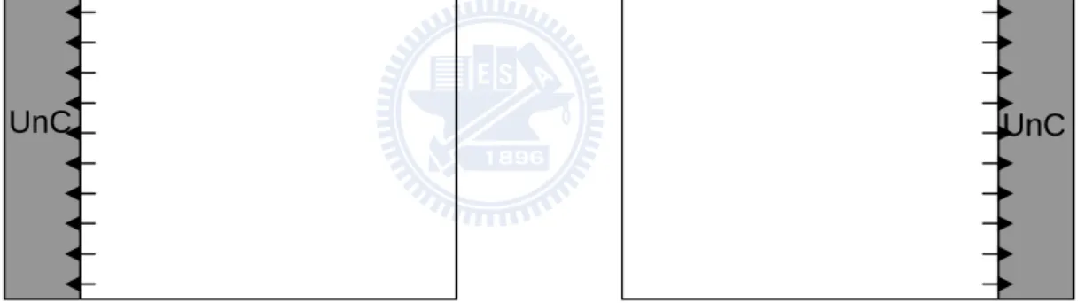
Theoretically, for the pixels in the uncovered areas, we also have to find four-neighbor reliable depth pixel. However, the uncovered area exists at the left side of the left view image or exists at the right side of the right view image. There is only one side reference for each pixel in uncovered areas. The uncovered pixels in left view only have reliable depth pixel at right side and the uncovered pixels in right view only have reliable depth pixel at left side. Therefore, the four-neighbor reliable depth pixel search can be reduced and the interpolation can be removed in depth refining process for the uncovered pixels. This process is shown in Figure 3-14. The uncovered pixel in left view copies the depth value of the right reliable depth pixel as its depth value and the uncovered pixel in right view copies the depth value of the left reliable depth pixel as its depth value.

Figure 3-14: Refinement of uncovered area.

Left: depth map of left view, Right: depth map of right view.

3.2.4 Results of depth refinement

The results of depth refinement algorithm are presented in Figure 3-15 to Figure 3-17. The original depth map at the left side of each figure is generated by DERS [16] with modified depth estimation error function. The depth map at the right side of each figure is the

UnC UnC

(40)

refined depth map.

Figure 3-15 shows the results of sequence BookArrival after applying depth refinement algorithm, Figure 3-15(a) is the original depth map and Figure 3-15(b) is the refined depth map. The depth values around the left boundary of the sitting man and the stone lion are refined with the reasonable values. The uncovered area at left side is also refined with reasonable guess.

(a) (b) Figure 3-15: Results of sequence BookArrival after applying depth refinement algorithm.

(a) The original depth map of the left view, (b) The refined depth map of the left view

Figure 3-16 shows the results of depth refinement of sequence Lovebird1. The quality of depth map is not improved obviously because the unreliable depth pixels are not as many as that in sequence BookArrival. The shape of the foreground is sharper after applying the proposed method. Figure 3-16(a) is the original depth map, Figure 3-16(b) is the refined depth map.

(41)

(a) (b) Figure 3-16: Results of sequence Lovebird1 after applying depth refinement algorithm.

(a) The original depth map of the left view, (b) The refined depth map of the left view

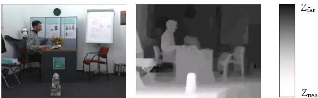
The results of depth refinement of sequence Newspaper are shown in Figure 3-17. The quality of depth map is improved obviously, especially in uncovered areas. The improvement will affect the quality of synthesized view significantly. The results of view synthesis are discussed in the next chapter. Figure 3-17(a) is the original depth map, Figure 3-17(b) is the refined depth map.

(a) (b) Figure 3-17: Results of sequence Newspaper after applying depth refinement algorithm.

(42)

3.3 Modified View Synthesis Algorithm

We have proposed a reliable weighted interpolation function in section 3.2. Similar idea can be used in view synthesis process. The view synthesis algorithm in [3] will generate two different mapped virtual images and then these two images are merged according to the ratio of left and right baseline distances. The pixels in these two images can be mapped from reliable depth pixels or from unreliable depth pixels. We can use the same reliable weighting to recalculate the weighting factor for the image mapped from left view and the weighting factor for the image mapped from right view. The original weighting factors for the mapped image from left view WDLeft and the mapped image from right view WDRight are represented as

follows. Right Left Right Left Dis Dis Dis WD + = (11) Right Left Left Right Dis Dis Dis WD + = (12)

where DisRight and DisLeft are right baseline distance and left baseline distance, respectively.

If one of the mapped pixels is from reliable depth pixel and the other is from unreliable depth pixel, WDLeft and WDRight of the view synthesis algorithm [3] are then modified by the

following description. The weighting value WHighR and WLowR used in the depth refinement

step can be used here. WHighR and WLowR are the weighting values of high reliability reliable

depth pixel and low reliability reliable depth pixel, respectively. WDLeft and WDRight are

multiplied by WHighR and WLowR as follows:

for the mapped pixels from left view or right view if the mapped pixel is from reliable depth pixel

(43)

HighR Direction Direction WD W WD '= ⋅ ₍₁₃₎ else LowR Direction Direction WD W WD '= ⋅ (14)

where “Direction” in lower index can be either Left or Right.

The new weighting factors for the mapped pixels from left view and the mapped pixels from right will be:

' ' ' " Right Left Right Left WD WD WD WD + = ₍₁₅₎ ' ' ' " Right Left Left Right WD WD WD WD + = ₍₁₆₎

(44)

Chapter 4. Results of View Synthesis

The quality of the refined depth map will be evaluated by results of view synthesis. If the refined depth map has better resolution, the synthesized virtual views shall also have better quality. The simulation results will be compared subjectively and objectively. The subjective comparison is presented in section 4.1 and the objective comparison is described in section 4.2. In objective results comparison, we will compare our method to [23]. The virtual views generated by our method in section 4.1 and 4.2 are using the refined depth map and synthesized by the reliable weighted view synthesis algorithm. Except for the comparison of whole image, we emphasize the improvement of reliable weighted view synthesis in section 4.3.

The test sequences are from [26]. The reference views used to perform the depth estimation and the synthesized views for the evaluation are listed in Table 4-1. The number of synthesized frames is 100; all test sequences synthesize the same number of frames. The original depth map in this chapter is the depth map generated by DERS [16] with modified depth estimation error function.

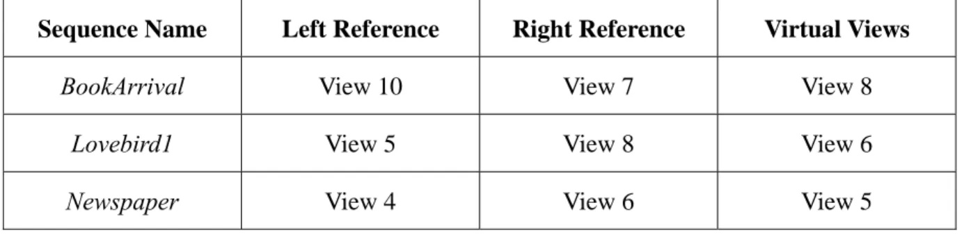
Table 4-1: Test sequences and virtual views to be synthesized

Sequence Name Left Reference Right Reference Virtual Views

BookArrival View 10 View 7 View 8

Lovebird1 View 5 View 8 View 6

(45)

4.1 Subjective Results Comparison

The visual quality of refined depth map is shown in section 3.2. It shows that depth map is more precise around object boundaries. The visual quality of synthesized virtual views should be improved if the refined depth map is used. The visual quality improvement of synthesized virtual views is exhibited in this section.

4.1.1 Results of BookArrival

Figure 4-1 to 4-4 shows the simulation results of sequence BookArrival. Figure 4-1 is the result of frame number 58. Figure 4-1(a) is the original video data, 4-1(b) is the result generated with original depth map and VSRS [3], 4-1(c) is the result generated with refined depth map and proposed view synthesis algorithm. The green rectangle area is enlarged in figure 4-2 to see the visual quality improvement clearly. Figure 4-2(b) is the green rectangle area of figure 4-1(b), figure 4-2(c) is the green rectangle area of figure 4-1(c). The noises around objects boundaries are removed and object in occluded area is synthesized more correctly (e.g., the earphone in the left most red ellipse) when our method is applied. The improved areas are highlighted with red ellipse. Figure 4-3 is the result of frame number 73. Figure 4-3(a) is the original video data, 4-3(b) is the result generated with original depth map and VSRS, 4-3(c) is the result generated with refined depth map and proposed view synthesis algorithm. Figure 4-4(a), 4-4(b), and 4-4(c) are the green rectangle areas of figure 4-3(a), 4-3(b), and 4-4(c). The improved areas are also highlighted in figure 4-4.

(46)

(a)

(b) (c) Figure 4-1: Experimental results of frame #58 of sequence BookArrival.

(a) Original video, (b) virtual view generated with original depth map and VSRS, (c) virtual view generated with refined depth map and proposed view synthesis algorithm.

(47)

(b) (c) Figure 4-2: Enlarged results from figure 4-1.

(a)

(b) (c) Figure 4-3: Experimental results of frame #73 of sequence BookArrival.

(48)

(a)

4.1.2 Results of Lovebird1

The results of sequence Lovebird1 are shown in figure 4-5 to 4-8. The visual quality around the boundaries of the foreground walking people is improved and the shapes of the man and woman are sharper. Red ellipses highlight the improved areas. Figure 4-5 and 4-6 are the results of frame number 6. Figure 4-7 and 4-8 are the results of frame number 35. The arrangement of sub-figures is the same as the results of sequence BookArrival. Sub-figure (a) is the original video data, (b) is the result generated from original depth map and VSRS, and

(49)

(c) is the result generated from refined depth map and proposed view synthesis algorithm. Figure 4-5 and 4-7 are the results of whole image, figure 4-6 and 4-8 are the enlarged results from figure 4-5 and 4-7, respectively.

(a)

(b) (c) Figure 4-5: Experimental results of frame #6 of sequence Lovebird1.

(50)

(a)

(51)

(b) (c) Figure 4-7: Experimental results of frame #35 of sequence Lovebird1.

(a)

(52)

4.1.3 Results of Newspaper

The same improvement of visual quality can be found in sequence Newspaper, the boundaries of objects are clearer when proposed method is applied. The results are shown in figure 4-9 and 4-10. Figure 4-9 is the results of frame number 0, the green rectangle areas in figure 4-9 are enlarged in figure 4-10. Again, sub-figure (a) is the original video data, (b) is the result generated from original depth map and VSRS, and (c) is the result generated from refined depth map and proposed view synthesis algorithm. There is another noticeable improvement in the synthesized image, our method has better quality of the red ellipse area. This is because of our method refined the uncovered area of depth map.

(53)

(b) (c) Figure 4-9: Experimental results of frame #0 of sequence Newspaper.

(a) (b) (c) Figure 4-10: Enlarged results from figure 4-9.

(54)

4.2 Objective Results Comparison

In this section, the results of objective comparison are obtained by PSNR and Peak Signal to Perceptual Noise Ratio (PSPNR) tool. PSPNR is a tool for view synthesis quality evaluation. There is a mode for excluding left-most and right-most N pixels in PSPNR calculation. All sequences are tested with 100 frames and the results are averaged. We have calculated the 30-pixels exclusion results and no pixel exclusion results. Both results will be shown in the following description. The “DERS+VSRS” in the tables and figures stands for the results of the DERS [16] with modified depth estimation error function and the view synthesis tool VSRS [3], while “[23]” means the results from the original depth map and the method described in [23]. “Proposed” is for the results of the proposed algorithm with

WHighR=0.75 and WLowR=0.25.

4.2.1 Results of BookArrival

Table 4-2 shows 30 pixels excluded PSNR and PSPNR results of synthesized view 8 of sequence BookArrival. The results are the average value of 100 frames. The test results of 30-pixel exclusion show that proposed method has 1.02dB improvement in PSNR and 2.45dB improvement in S_PSPNR. Figure 4-11, 4-12, and 4-13 are PSNR of each frame, S_PSPNR of each frame, and T_PSPNR of each frame, respectively. It shows that proposed method improves quality of each frame of virtual view. The drop around frame number 30 is caused by a man coming from right side.

(55)

Table 4-2: PSNR and PSPNR results of virtual view 8 of sequence BookArrival (30 pixels excluded).

PSNR S_PSPNR T_PSPNR

N-pixel

exclusion DERS+VSRS [23] Proposed DERS+VSRS [23] Proposed DERS+VSRS [23] Proposed

30-pixels exclusion 35.56 35.62 36.59 39.51 39.54 41.96 47.82 47.66 51.69 0 10 20 30 40 50 60 70 80 90 100 33 34 35 36 37 38 P S NR( d B ) Frame Number

BookArrival - Frame PSNR (30 pixels excluded)

DERS+VSRS [23]

Proposed

Figure 4-11: Frame PSNR of virtual view 8 of sequence BookArrival (30 pixels excluded).

0 10 20 30 40 50 60 70 80 90 100 34 35 36 37 38 39 40 41 42 43 44 S-P SPN R (dB) Frame Number

BookArrival - Frame S-PSPNR (30 pixels excluded)

DERS+VSRS [23]

Proposed

Figure 4-12: Frame S_PSPNR of virtual view 8 of sequence BookArrival (30 pixels excluded).

(56)

0 10 20 30 40 50 60 70 80 90 100 42 44 46 48 50 52 54 56 T -PS PN R (d B) Frame Number

BookArrival - Frame T-PSPNR (30 pixels excluded)

DERS+VSRS [23]

Proposed

Figure 4-13: Frame T_PSPNR of virtual view 8 of sequence BookArrival (30 pixels excluded).

Table 4-3 shows no pixel excluded PSNR and PSPNR results of synthesized view 8 of sequence BookArrival. All results are lower than 30 pixels exclusion because of the uncovered areas at left side or right side in the depth map. Even though the test results of no exclusion are lower than the results of 30 pixels exclusion, proposed method still has 1.58dB improvement in PSNR and 2.20dB improvement in S_PSPNR. The amount of improvement in PSNR is larger than the result of 30 pixels excluded PSNR. This is because proposed method refines uncovered areas at left and right side of original depth map. Figure 4-14, 4-15, and 4-16 are PSNR of each frame, S_PSPNR of each frame, and T_PSPNR of each frame, respectively. The trends of curves in the figures are similar to the results of 30 pixels exclusion.

(57)

Table 4-3: PSNR and PSPNR results of virtual view 8 of sequence BookArrival (No pixel excluded).

N-pixel

No pixels exclusion 31.99 32.01 33.57 33.44 33.44 35.64 47.70 47.54 50.88 0 10 20 30 40 50 60 70 80 90 100 30 30.5 31 31.5 32 32.5 33 33.5 34 34.5 35 PS N R (dB) Frame Number

BookArrival - Frame PSNR (No pixel excluded)

DERS+VSRS [23]

Proposed

Figure 4-14: Frame PSNR of virtual view 8 of sequence BookArrival (No pixel excluded).

0 10 20 30 40 50 60 70 80 90 100 31 32 33 34 35 36 37 S-PSPN R (d B ) Frame Number

BookArrival - Frame S-PSPNR (No pixel excluded)

DERS+VSRS [23]

Proposed

(58)

0 10 20 30 40 50 60 70 80 90 100 40 45 50 55 T -P SPN R (d B ) Frame Number

BookArrival - Frame T-PSPNR (No pixel excluded)

DERS+VSRS [23]

Proposed

Figure 4-16: Frame T_PSPNR of virtual view 8 of sequence BookArrival (No pixel excluded).

4.2.2 Results of Lovebird1

Table 4-4 shows 30 pixels excluded PSNR and PSPNR results of synthesized view 6 of sequence Lovebird1. The improvement in PSNR is 0.30dB and the improvement in S_PSPNR is 0.72dB. Because refined depth map has a little improvement that is shown in section 3.2.3. The improvement of quality of virtual view is not obvious as sequence BookArrival. Figure 4-17, 4-18, and 4-19 present the PSNR, S_PSPNR, and T_PSPNR frame by frame.

.

Table 4-4: PSNR and PSPNR results of virtual view 6 of sequence Lovebird1 (30 pixels excluded).

N-pixel

30-pixels

(59)

0 10 20 30 40 50 60 70 80 90 100 30 30.5 31 31.5 32 PS N R (d B ) Frame Number

Lovebird1 - Frame PSNR (30 pixels excluded)

DERS+VSRS [23]

Proposed

Figure 4-17: Frame PSNR of virtual view 6 of sequence Lovebird1 (30 pixels excluded).

0 10 20 30 40 50 60 70 80 90 100 33.5 34 34.5 35 35.5 36 36.5 S-PSPN R (d B ) Frame Number

Lovebird1 - Frame S-PSPNR (30 pixels excluded)

DERS+VSRS [23]

Proposed

(60)

0 10 20 30 40 50 60 70 80 90 100 44 46 48 50 52 54 56 58 T -P S P NR( d B ) Frame Number

Lovebird1 - Frame T-PSPNR (30 pixels excluded)

DERS+VSRS [23]

Proposed

Figure 4-19: Frame T_PSPNR of virtual view 6 of sequence Lovebird1 (30 pixels excluded).

Table 4-5 shows no pixel excluded PSNR and PSPNR results of synthesized view 6 of sequence Lovebird1. The improvement in PSNR is 0.27dB and the improvement in S_PSPNR is 0.60dB. Figure 4-20, 4-21, and 4-22 present the PSNR, S_PSPNR, and T_PSPNR frame by frame. The figures are similar to the results of 30 pixels exclusion.

Table 4-5: PSNR and PSPNR results of virtual view 6 of sequence Lovebird1 (No pixel excluded).

N-pixel

30-pixels

(61)

0 10 20 30 40 50 60 70 80 90 100 29.5 30 30.5 31 31.5 PSN R (d B) Frame Number

Lovebird1 - Frame PSNR (No pixel excluded)

DERS+VSRS [23]

Proposed

Figure 4-20: Frame PSNR of virtual view 6 of sequence Lovebird1 (No pixel excluded).

0 10 20 30 40 50 60 70 80 90 100 32.5 33 33.5 34 34.5 35 35.5 S-PS PN R (dB) Frame Number

Lovebird1 - Frame S-PSPNR (No pixel excluded)

DERS+VSRS [23]

Proposed

(62)

0 10 20 30 40 50 60 70 80 90 100 46 48 50 52 54 56 58 T-PSP N R (dB) Frame Number

Lovebird1 - Frame T-PSPNR (No pixel excluded)

DERS+VSRS [23]

Proposed

Figure 4-22: Frame T_PSPNR of virtual view 6 of sequence Lovebird1 (No pixel excluded).

4.2.3 Results of Newspaper

Table 4-6 shows 30 pixels excluded PSNR and PSPNR results of synthesized view 5 of sequence Newspaper. The improvement in PSNR is 0.75dB and the improvement in S_PSPNR is 1.74dB. Figure 4-23, 4-24, and 4-25 present the PSNR, S_PSPNR, and T_PSPNR frame by frame. The results show that proposed method has a significant improvement.

Table 4-6: PSNR and PSPNR results of virtual view 5 of sequence Newspaper (30 pixels excluded).

N-pixel

30-pixels

(63)

0 10 20 30 40 50 60 70 80 90 100 30 30.5 31 31.5 32 32.5 33 P S NR( d B ) Frame Number

Newspaper - Frame PSNR (30 pixels excluded)

DERS+VSRS [23]

Proposed

Figure 4-23: Frame PSNR of virtual view 5 of sequence Newspaper (30 pixels excluded).

0 10 20 30 40 50 60 70 80 90 100 33 33.5 34 34.5 35 35.5 36 36.5 37 37.5 38 S-PSPN R (d B) Frame Number

Newspaper - Frame S-PSPNR (30 pixels excluded)

DERS+VSRS [23]

Proposed

(64)

0 10 20 30 40 50 60 70 80 90 100 44 45 46 47 48 49 50 51 52 53 T -PSPN R (d B) Frame Number

Newspaper - Frame T-PSPNR (30 pixels excluded)

DERS+VSRS [23]

Proposed

Figure 4-25: Frame T_PSPNR of virtual view 5 of sequence Newspaper (30 pixels excluded).

Table 4-7 shows no pixel excluded PSNR and PSPNR results of synthesized view 5 of sequence Newspaper. The improvement in PSNR is 4.06dB and the improvement in S_PSPNR is 6.68dB. Figure 4-26, 4-27, and 4-28 present the PSNR, S_PSPNR, and T_PSPNR frame by frame. The results of depth refinement that shown in figure 3-13 can explain the reason why PSNR and S_PSPNR have a huge improvement. The results of depth refinement of uncovered depth pixels in the right reference view correct a large area of unreliable depth. The calculation of PSNR and PSPNR is including all pixels in the image, the bad depth values in the original depth map drop the results of PSNR and PSPNR.

Table 4-7: PSNR and PSPNR results of virtual view 5 of sequence Newspaper (No pixel excluded).

N-pixel

30-pixels

(65)

0 10 20 30 40 50 60 70 80 90 100 26 27 28 29 30 31 32 33 PSN R (d B) Frame Number

Newspaper - Frame PSNR (No pixel excluded)

DERS+VSRS [23]

Proposed

Figure 4-26: Frame PSNR of virtual view 5 of sequence Newspaper (No pixel excluded).

0 10 20 30 40 50 60 70 80 90 100 28 30 32 34 36 38 S-PSPN R (d B) Frame Number

Newspaper - Frame S-PSPNR (No pixel excluded)

DERS+VSRS [23]

Proposed

針對多視角視訊合成之景深修正演算法

國

立

交

通

大

學

多媒體工程研究所

碩

士

論

文

針 對 多 視 角 視 訊 合 成 之 景 深 修 正 演 算 法

A depth refinement algorithm for multi-view video synthesis

研 究 生：石新嘉

指導教授：蕭旭峯 教授

針對多視角視訊合成之景深修正演算法

摘要

A depth refinement algorithm for multi-view video synthesis

Abstract

Acknowledgement

Contents

-List of Tables

-List of Figures

-Chapter 1. Introduction

Chapter 2. Related Work

2.1 Depth Estimation

2.1.1 Stereo matching

2.1.2 Segment-based depth estimation

2.1.3 Pixel-based depth estimation

2.1.4 Temporal consistency for depth estimation

2.2 View Synthesis

2.2.1 View synthesis algorithm

2.2.2 Improving view synthesis for multi-view video

2.2.3 View synthesis for stereo vision

Chapter 3. Proposed Depth Refinement

Algorithm

3.1 Camera Setting for Depth Estimation

3.1.1 Camera setting in related works

3.1.2 Stereo camera setting

3.2 Depth Refinement Algorithm

3.2.1 Depth consistency check

3.2.2 Occlusion detection

3.2.3 Depth refinement

a

b

c

d

: Unreliable Area

: Reliable Area

: Reliable Area

: Reliable Area

: Unreliable Area

: Reliable Area

: Reliable Area

: Reliable Area

3.2.4 Results of depth refinement

3.3 Modified View Synthesis Algorithm

Chapter 4. Results of View Synthesis

4.1 Subjective Results Comparison

4.1.1 Results of BookArrival

4.1.2 Results of Lovebird1

4.1.3 Results of Newspaper

4.2 Objective Results Comparison

4.2.1 Results of BookArrival

4.2.2 Results of Lovebird1

4.2.3 Results of Newspaper

針對多視角視訊合成之景深修正演算法

研究生：石新嘉

指導教授：蕭旭峯教授

_{: Unreliable Area}