關於統計上顯著性差異模式探索之研究

國

立

交

通

大

學

資訊科學與工程研究所

碩

士

論

文

關於統計上顯著性差異模式探索之研究

A Study of Statistically Significant Difference Pattern

Detection

研 究 生：羅仁杰

指導教授：曾憲雄 博士

關 於 統 計 上 顯 著 性 差 異 模 式 探 索 之 研 究

A Study of Statistically Significant Difference Pattern Detection

研 究 生：羅仁杰 Student：Ren-Jei Luo

指導教授：曾憲雄 博士 Advisor：Dr. Shian-Shyong Tseng

國 立 交 通 大 學

資 訊 科 學 與 工 程 研 究 所

碩 士 論 文

A Thesis

Submitted to Institute of Computer Science and Engineering College of Computer Science

National Chiao Tung University in partial Fulfillment of the Requirements

for the Degree of Master

in

Computer Science June 2006

Hsinchu, Taiwan, Republic of China

關於統計上顯著性差異模式探索之研究

研究生 : 羅仁杰 指導教授 : 曾憲雄博士 國 立 交 通 大 學 資 訊 科 學 研 究 所

摘要

在傳統的問卷分析中，因為傳統的分析方式是一個非常依賴經驗並且不斷重 複嘗試的分析方法，所以很容易發生顯著性差異被忽略或是未被認知的情況，進 而影響到資料分析的結果。例如數位落差分析者可能著重於性別對成績的影響， 而忽略到其它可能的因素或者覺得該因素不重要，例如父母親的教育程度對成績 也會有影響。我們將此問題稱為「顯著差異未被認知問題」。 為了解決顯著差異未被認知問題，我們希望將原本依賴經驗法則的分析方式 轉換為一個主動發現的分析方式。所以我們需要更為豐富的資料和一個更具彈性 的分析方法。為了達到這些目的，在這裡我們導入了資料倉儲技術。資料倉儲除 了可以對資料做完善的處理，它還提供了方便的線上分析工具-OLAP。但是 OLAP 本身的設計並不是用來解決假設未被認知問題，所以我們致力研究如何在此多維 多層的架構之下探索具有統計上顯著性意義的模式來解決假設未被認知問題。我 們為此訂定了一個完善的定義並稱之為「顯著性差異模式探索問題(SDPD)」。因 為導入了資料倉儲技術後會引發資料量過大和探索維度過於複雜的問題，所以我 們也提供了一套貪婪演算法 WISDOM 來解決 SDPD 問題。這個貪婪演算法 WISDOM 包含二個主要程序，一個是具有啟發式資料縮減程序可以有效的縮減資料量並對 資料做整理。另一個顯著性差異模式探勘程序則可以有效的判斷單一維度例如性 別對單一量值例如成績是否存在顯著性差異。最後再將探索出來的模式交由專家 去做參考與使用。 關鍵字：資料探勘、顯著性差異、資料倉儲、線上分析處理、數位落差

A Study of Statistically Significant

Difference Pattern Detection

Student: Ren-Jei Luo Advisor: Dr. Shian-Shyong Tseng

Department of Computer and Information Science National Chiao Tung University

Abstract

In the traditional Questionnaire Analysis, there exists a problem that researchers may miss or ignore some causes because the traditional analysis usually is performed in an experiential try-and-error manner. For example, the digital divide researchers may focus on the difference in the grade between different genders. But they may miss other causes of the difference in the grade (e.g., parents’ education, living locations, parents’ vocations). These causes may also lead to the difference in grade. We name it “Significant Difference Unawareness Problem”.

In order to solve the Significant Difference Unawareness Problem, we propose a semi-automatic discovery-based analysis method instead of the traditional hypothesis-based analysis manner. Since a more flexible analysis on richer data is required in our method. Hence, we apply the data warehousing technique is applied. We discuss how to detect the entire interesting pattern that implies the causes of the difference on the multi-dimensional data structure, and define this problem as Significant Difference Pattern Detection (SDPD). After applying the data warehousing, some problems must be solved: the data size is huge and the combination of dimensions is very complex. So we propose a greedy algorithm, WISDOM (Wisely Imaginable Significant Difference Observation Mechanism), to solve the SDPD problem. The WISDOM includes two major processes: (1) Data Reduction Process. The Data Reduction Process has a sensitive-less data filtering heuristic that is useful to reduce the data size. (2) SD Pattern Mining Processes. The SD Pattern Mining has a significant difference pattern determination heuristic that is

effective to determinate if there exists a significant difference in a single dimension versus a single measure.

Keyword：Data Mining, Significant Difference, Data Warehousing, On-Line Analytic Processing (OLAP), Digital Divide

致謝

首先要感謝的是我的指導教授，曾憲雄博士。在我碩士班這二年的時間當 中，曾教授相當細心與耐心的指導我研究的方法；並從老師的身上學習到許多研 究的方法與態度，寶貴的經驗讓我獲益良多，不甚感激！因此也讓我能順利的完 成此篇論文。同時也感謝我的口試委員，洪宗貝教授，葉耀明教授以及彭文志教 授所給予的寶貴意見，讓我的論文研究能夠更有價值。 接下來要感謝曲衍旭學長以及翁瑞鋒學長。在這兩年期間讓我學會許多理論 知識及實務技巧，並給予我許多論文上的寶貴意見，協助我論文上的修改工作， 使得這篇論文能夠順利的完成。還有謝謝實驗室中的學長姐和各位同窗的夥伴們 以及其它在我身邊鼓勵我的朋友，陪伴我渡過這充實的碩士生涯，並在我感到挫 折時給我支持的力量，讓我很快的振作起來。 另外要感謝我的父母親在背後默默地支持我完成我的學業，讓我可以安心的 做研究而不需要煩惱生活上的問題。最後要特別感謝我的女朋友湘婷，在我身邊 不時地關心我、照顧我。也讓我能夠自信地、樂觀地面對一切難題。日後，我會 更加努力的繼續向前進！

Table of Contents

摘要... I ABSTRACT ...II 致謝... IV TABLE OF CONTENTS ... V LIST OF FIGURES... VI LIST OF TABLES ...VII

CHAPTER 1. INTRODUCTION ...1

CHAPTER 2. RELATED WORK ...5

2.1. QUANTITATIVE RESEARCH...5

2.2. INDICATOR...7

2.3. DEVIATION DETECTION...9

2.4. FEATURE SELECTION...10

CHAPTER 3. PROBLEM DEFINITION ...12

3.1. DATA WAREHOUSE...12

3.2. SIGNIFICANT DIFFERENCE PATTERN...14

3.3. SIGNIFICANT DIFFERENCE PATTERN DETECTION...16

CHAPTER 4. WISDOM: WISELY IMAGINABLE SIGNIFICANT DIFFERENCE OBSERVATION MECHANISM...18

4.1. DATA REDUCTION STEP...20

4.2. SDPMINING STEP...25

4.3. SDPRANKING STEP...37

CHAPTER 5. EXPERIMENT ...39

5.1. ACCURACY AND RECALL OF THE WISDOM...41

5.2. PERFORMANCE OF THE WISDOM...46

5.3. EXPERIMENTS SUMMARY...50

CHAPTER 6. CONCLUSION ...51

List of Figures

FIGURE 4.1:THE FLOWCHART OF WISDOM ALGORITHM...19

FIGURE 4.2:THE NORMAL DISTRIBUTION...21

FIGURE 4.3:THE SCORE AND RANGE OF ATTRIBUTE REGION...28

FIGURE 4.4:THE RESULT AFTER SEARCHING THE FIRST LEVEL IN...33

FIGURE 4.5:THE RESULT AFTER SEARCHING THE SECOND LEVEL IN...34

FIGURE 4.6:THE RESULT AFTER SEARCHING THE FIRST LEVEL IN...35

FIGURE 4.7:THE RESULT AFTER SEARCHING THE SECOND LEVEL IN...36

FIGURE 5.1THE DIGITAL DIVIDE DATA WAREHOUSE (數位落差問卷資料庫) ...40

FIGURE 5.2THE STAR SCHEMA OF THE ELEMENTARY SCHOOL DATA CUBE (國小問卷結果) OF DIGITAL DIVIDE DATA WAREHOUSE...41

FIGURE 5.3THE RESULTS OF THE NINETEEN DIMENSIONS VERSUS MEASURE SUM11_16 USING SPSS....42

FIGURE 5.4THE ACCURACY AND RECALL OF WISDOM. Γ=0.1~2 INCREASING BY 0.1 Β=0, DEPTH=1...43

FIGURE 5.5THE ACCURACY AND RECALL OF WISDOM. Γ=0.1~0.32 INCREASING BY 0.01 Β=0, DEPTH=1 ...44

FIGURE 5.6THE ACCURACY AND RECALL OF WISDOM Γ=0.16, DEPTH=1,Β=0~2 INCREASING BY 0.1....45

FIGURE 5.7THE EXECUTION TIME OF WISDOM Γ=0.16,DEPTH=1,Β=0~2 INCREASING BY 0.1...46

FIGURE 5.8THE ACCURACY AND EXECUTION TIME OF WISDOM.Γ=0.16, DEPTH=1,Β=0~2 INCREASING BY 0.1 ...47

FIGURE 5.9THE EXECUTION TIME OF WISDOM. Γ=3, DEPTH=1~5 INCREASING BY 1,Β=0...48

FIGURE 5.10THE RELATIONSHIP BETWEEN NUMBER OF DIMENSIONS AND EXECUTION TIME.Γ=3, DEPTH=3,Β=0. ...49

FIGURE 5.11THE RELATIONSHIP BETWEEN CONCEPT HIERARCHY AND EXECUTION TIME. Γ=3, DEPTH=3,Β=0. ...50

List of Tables

TABLE 3.1:THE 9 RECORDS OF EXAMPLE1...14

TABLE 4.1:THE WISDOM ALGORITHM...19

TABLE 4.2:THE RECORDS WITH ATTRIBUTE REGION AND MEASURE MATH_GRADE...22

TABLE 4.3:THE RECORDS AFTER APPLYING SENSITIVE-LESS DATA FILTERING HEURISTIC...22

TABLE 4.4.THE RECORDS AFTER APPLYING SENSITIVE DATA CATEGORIZING HEURISTIC...23

TABLE 4.5:THE DATAREDUCTION ALGORITHM...24

TABLE 4.6:THE SDPMINING ALGORITHM...32

Chapter 1. Introduction

Social science research is the use of scientific methods to investigate human behavior and social phenomenon [3]. However, the population of human society is generally very huge. Since it is impossible for social science researchers to thoroughly observe the huge population for a behavior or a phenomenon, they usually use questionnaire survey instead of investigating the whole population.

Questionnaire survey is usually done by selecting some representative samples from population according to the sampling methods. For analyzing the questionnaire data, researchers can use not only descriptive statistics methods, but also inferential statistics methods to infer the real human behavior and social phenomenon.

In the questionnaire analysis, finding whether there is significant difference between two or more groups in one measure is one of the major problems in researches. For example, in a survey of junior high school students’ current status, “Is there significant difference between different genders’ IQ?” and “Is there significant difference between the mathematics grades of different areas in Taiwan?” are two interesting phenomenon that researchers want to know. [3] categorized the research questions into degree of relationship among variables, significance of group differences, prediction of group membership, and structure, which significance of group differences is used to find the significant difference. Therefore, finding possible

significant difference between different groups is a very important research issue.

However, finding possible significant difference namely is difficult for social science researchers. In our observation, there are two main causes may lead to this issue.

The first cause is that researchers find the significant difference by their intuition and experience. For example, a junior researcher might consider that there is significant difference between different genders’ IQ. She/He could make a hypothesis, “There will be difference between different genders’ IQ,” and then use inferential statistics method to test this hypothesis. This is basically a hypothesis-based search method. Once the hypotheses are not made the significant difference can not be found even if it really exists. However, senior researchers might find it easier because of their rich experiences.

The second cause is that the original questionnaire data may be not good enough to find the significant differences. For example, in the survey of junior high school students’ current status, the student’s resident dimension doesn’t have granularity, and just contains the region attribute. If there is no significant difference between the mathematics grades of different regions, the researcher can just say there is no significant difference between the mathematics grades of different regions. However, if the researchers combine their collected data with secondary data which are collected by other researches [23] like the government official statistical data, geographic information, or other researches data, and assume the student’s resident

dimension has granularity, they would drill down the dimension to find whether there is significant difference between the mathematics grades of different cities.

In order to overcome the Significant Difference Unawareness issue, we apply data warehousing technology to integrate and maintain the questionnaire data and secondary data, and use a discovery-based search method to find the possible significant differences from the data warehouse semi-automatically. Data warehouse, which has subject-oriented, integrated, time-variant, and nonvolatile features, is a repository of integrated information, available for queries and analysis [23]. It also supports OLAP systems which can be used to query and explore the data at different granularities. Furthermore, a discovery-based search method is used to find the possible significant differences from data warehouse before analyzing the questionnaire data. According to these results, researchers can briefly understand where the possible significant differences are, and they can easily explore the data using OLAP systems.

In this thesis, the Significant Difference Pattern is formally defined first. Next, a Significant Difference Pattern Detection problem (SDPD problem), which is the

problem of finding all the possible significant difference from the data warehouse, is proposed. According to our observation of Significant Difference Pattern, a heuristic about the property of Significant Difference Pattern is proposed; besides, a greedy algorithm based on this heuristic is proposed to solve the Significant Difference Pattern Detection problem.

The rest of this thesis is organized as follows. Chapter 2 briefly introduces the related researches about fining significant difference. In Chapter 3, the clear definitions of Significant Difference Pattern and Significant Difference Pattern Detection problem are given. A greedy algorithm, WISDOM, is proposed in Chapter 4 to solve the Significant Difference Pattern Detection problem based on the heuristics. Moreover, some experiment results of the WISDOM algorithm are shown in Chapter 5 .Finally, we make conclusions and describe the future works in Chapter 6.

Chapter 2. Related Work

According to our survey, there are no related researches on this significant difference pattern detection problem. In this chapter, we introduce some related work: The problem of the traditional quantitative research, the indicator of data warehouse to indicator the difference, the deviation detection to detect the pattern that differ from trend and the feature selection is also not a solution for this problem.

2.1. Quantitative research

Quantitative research techniques [11] [23] are part of primary research and the data which are reported numerically can be collected through structured interviews, experiments, or surveys.

Quantitative research is all about quantifying relationships between variables. Variables are things like weight, performance, time, and treatment. You measure variables on a sample of subjects, which can be tissues, cells, animals, or humans. You express the relationship between variable using effect statistics, such as correlations, relative frequencies, or differences between means.

“Hypothesis Testing” is the most popular statistics method [11] to analyze the relationship between variables. And the researchers are most concerned about the differences between means, because the difference can immediately and effectively indicate the causality of the subject. If some variable like the gender of students versus the grades of students has a difference which is a statistical significant at a given 1-α confident level, then we said that there is a significant difference between the gender of students versus the grades.

In the traditional quantitative research, the researchers will firstly propose several hypotheses of the subject according to their experiences, and then test the hypotheses one by one to check if there exists a statistic significant in some hypotheses. Hence, it calls a try-and-error manner. The quality of the result using the manner, of course, is in accordance with the hypotheses made by the researchers.

Furthermore, the quantitative research researcher’s aim is to determine the relationship between one thing and another in a population. Quantitative research designs are either descriptive (subjects usually measured once) or experimental (subjects measured before and after a treatment). An experiment establishes causality. For an accurate estimate of the relationship between variables, a descriptive study usually needs a sample of hundreds or even thousands of subjects; an experiment, especially a crossover, may need only tens of subjects. The estimate of the relationship is unlikely to be biased if researchers have a high participation rate in a sample selected randomly from a population. In several statistical experiments, bias is also unlikely if subjects are randomly assigned to treatments, and if subjects and

researchers are blind to the identity of the treatments. In all studies, subject characteristics can affect the relationship you are investigating and limit their effect either by using a less heterogeneous sample of subjects or preferably by measuring the characteristics and including them in the analysis. In an experiment, they try to measure variables that might explain the mechanism of the treatment. In an unblended experiment, such variables can help define the magnitude of any placebo effect.

2.2. Indicator

Indicator [17] [18] is not used in a discovery-based analysis but is a useful tool to assist exploring the data cube of the data warehouse by OLAP. In order to implement indicators, a complete datacube should be constructed. In real case, building datacubes is very time consuming [1] [2] [4] [5]. Hence, using indicators is a computational expensive task.

The data warehouse could consist with several datacubes or single datacube. For each datacube, it has several records and a star schema to describe the schema of the datacube’s structure. In other word, the star schema can describe the dimensions with concept hierarchy and some measures of the datacube. And, the data warehouse supports an analysis tool: On-Line Analytic Processing (OLAP) [2] [19] [22]. It is a useful tool assistant to user exploring the datacube. OLAP can organize and present data in various formats in order to accommodate the diverse needs of the different analysis approaches. OLAP server provides server operations for analyzing

multidimensional data cube:

Roll-up: the roll-up operation collapses the dimension hierarchy along a particular dimension(s) so as to present the remaining dimensions at a coarser level of granularity.

Drill-down: in contrast, the drill-down function allows users to obtain a more detailed view of a given dimension.

Slice: Here, the objective is to extract a slice of the original cube corresponding to a single value of a given dimension. No aggregation is required with option. Instead, server allows the user to focus on desired values.

Dice: A related operation is the dice. In this case, users can define a sub cube of the original space. In other words, by specifying value ranger on one or more dimensions, the user can highlight meaningful blocks of aggregated data.

Pivot: the pivot is a simple but effective operation that allows OLAP users to visualize cube values in more natural and intuitive ways

The data warehouse also supports another analysis tool: On-Line Analytical Mining (OLAM) [2] [6] [12]. It integrates OLAP, data mining and knowledge

discovering on multi-dimensional database structure into OLAM. Hence, OLAM is also called OLAP Data Mining. The OLAM supports several data mining tasks such as the concept description, mining association rules, classification & prediction, and time sequential analysis.

Typically, the data mining algorithm is performed on a single “data mining” table. This table is produced by using the transformations and aggregations on the base data. Often, we need to generate the single table. This transformation is a key part of the data mining process. Often, it is a manual process and the physically elapsed time for locating, migrating, and transforming data is the orders of magnitude greater than the involved computing time. It is important that effective tools are used to support this process.

However, neither the OLAP nor the OLAM is a discovery-based analysis tool, and it can not detect the significant difference pattern automatically or semi-automatically.

2.3. Deviation Detection

Deviation detection [13] is a research which aims to detect the pattern differed from the predict pattern. They use a mathematic mode to predict the trend of the measures. Then using the difference of the predict trend and measure to determinate

the deviation. For example, if we predict that the height of a man is taller than a woman. Then deviation detection will detect the pattern, there exists a woman is taller than the man. Similarly, if we predict the profit of products at may be $10,000. Then deviation detection will detect the pattern that there exists a product, cell phone, has a large deviation on the profit. It may be $15,000 or $5,000.

2.4. Feature Selection

Feature selection [6] [14] [15], also known as subset selection or variable selection, is a process commonly used in machine learning, wherein a subset of the features available from the data is selected for application of a learning algorithm. Feature selection is necessary either because it is computationally infeasible to use all available features, or because of problems of estimation when limited data samples (but a large number of features) are present. The latter problem is related to the so-called curse of dimensionality.

Simple feature selection algorithms are ad hoc, but there are also more methodical approaches. From a theoretical perspective, it can be shown that optimal feature selection for supervised learning problems requires an exhaustive search of all possible subsets of features of the chosen cardinality. If large numbers of features are available, this is impractical. For practical supervised learning algorithms, the search is for a satisfactory set of features instead of an optimal set. Many popular approaches are greedy hill climbing approaches. Such an approach evaluates a possible subset of

features and then modifies that subset to see if an improved subset can be found. Evaluation of subsets can be done many ways - some metric is used to score the features, and possibly the combination of features. Since exhaustive search is generally impractical, at some stopping point, the subset of features with the highest scores by the metric will be selected. The stopping point varies by algorithm.

Two popular metrics for classification problems are correlation and mutual information. These metrics are computed between a candidate feature (or set of features) and the desired output category.

In statistics the most popular form of feature selection is called stepwise regression. It is a greedy algorithm that adds the best feature (or deletes the worst feature) at each round. The main control issue is deciding when to stop the algorithm. In machine learning, this would typically be done by cross validation. In statistics, some criteria would be optimized.

Chapter 3. Problem Definition

In order to avoid the Significant Difference Unawareness issue, we first build a data warehouse by integrating the questionnaire data and secondary data, and then use a discovery-based search method to find the possible significant differences from the data warehouse semi-automatically. Next, the desired significant difference is defined as Significant Difference Pattern. Finally, a new discovery-based problem, Significant Difference Pattern Detection problem, is proposed.

3.1. Data Warehouse

The data structure of Data Warehouse, containing dimensions, measures, and records, generally represents in a form of star schema, snowflake schema, or fact constellation schema, where the star schema is the most basic one and the other two can be derived by star schema [2][4][10]. To simplify our discussion, in this thesis, Data Warehouse based on the star schema is used to represent the data.

DEFINITION 1: Data Warehouse

A Data Warehouse contains p dimensions, Dimension = {Di| i = 1…p}, q

measures, Measure = {Mi| i = 1…q}, and n records, Record = {Ri| i = 1…n}. Each

Aif(i)>. Each attribute Aij contains g(i, j) attribute values, Aij = {Vijk| k = 1…g(i, j)}.

Each measure Mi is a continuous value. Each record Ri is the tuple of (A11, …, A1f(1),

A21, …, A2f(2), …, Apf(p), M1, …, Mq).

■

The Data Warehouse of EXAMPLE 1 is built based upon a questionnaire survey data for all the elementary school students in Taiwan. In the rest of this thesis, all the examples are based on this Data Warehouse.

EXAMPLE 1:

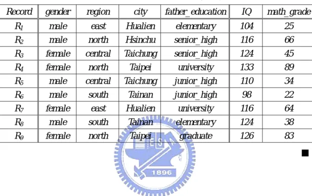
The Data Warehouse contains 3 dimensions, i.e. gender, resident_area, and father_education, 2 measures, i.e. IQ and math_grade, and 9 records. The detailed

structure of dimensions and measures are listed as follows, and the 9 records are listed in Table 3.1.

z Dimension = {gender, resident_area, father_education} „ gender = <gender>

‹ gender = {male, female} „ resident_area = <region, city>

‹ region = {north, central, south, east}

‹ city = {Taipei, Hsinchu, Taichung, Tainan, Hualien} „ father_education = <father_education>

university, graduate}

z Measure = {IQ, math_grade} z Record = {R1, R2, R3, …, R9}

Table 3.1: The 9 records of EXAMPLE 1

Record gender region city father_education IQ math_grade R1 male east Hualien elementary 104 25

R2 male north Hsinchu senior_high 116 66

R3 female central Taichung senior_high 124 45

R4 female north Taipei university 133 89

R5 male central Taichung junior_high 110 34

R6 male south Tainan junior_high 98 22

R7 female east Hualien university 116 64

R8 male south Tainan elementary 124 38

R9 female north Taipei graduate 126 83

■

3.2. Significant Difference Pattern

Significant difference, a specific term in statistics, represents two or more groups exist obviously different on a continuous variable. For representing clearly, a significant difference is defined as a Significant Difference Pattern.

DEFINITION 2: Significant Difference Pattern

significant difference at the given 1-α confidence level, where α is significance level in statistics. An SDP is composed by three parts: attribute part, condition part, and measure part. The attribute part contains one attribute, the condition part contains several “attribute equal to attribute value” pairs, and the measure part contains one measure. To simplify our discussion, assume there is only one “attribute equal to attribute value” pair in the condition part. The SDP is denoted as

(Aij | Axy = Vxyz) : Mk (3.1)

It means that there is significant difference between different attribute values of Aij on measure Mk for all the records satisfying Axy = Vxyz. Generally speaking, the

significance level α is set as 5% or 1%.

■

EXAMPLE 2:

Given the SDP:

(region | gender = male) : math_grade

This SDP means that, for all male, there is significant difference between different resident regions on math_grade.

■

3.3. Significant Difference Pattern Detection

The Data Warehouse and Significant Difference Pattern have been formally defined in the previous sections. In this section, we propose the problem of finding the possible SDPs from a given Data Warehouse as a new discovery-based problem, i.e. Significant Difference Pattern Detection problem.

DEFINITION 3: Significant Difference Pattern Detection problem

Given a Data Warehouse, α , β, γ , and Depth, finding the possible SDPs

from the Data Warehouse, where α is significance level, β is sensitivity ratio

threshold, γ is significance determination threshold, and Depth is search depth

threshold. In the following, the Significant Difference Pattern Detection problem is denoted as SDPD problem.

■

3.3.1 Difficulty of SDPD problem

question: What’s the complexity of the SDPD problem? In order to answer this question, let’s consider the following special case.

The special case has a well defined Multidimensional Database Structure. The Multidimensional Database Structure contains n dimensions and only 1 measure. Each dimension contains only 1 attribute. Each attribute has k values. If someone wants to find all the Significant Difference Pattern in this Multidimensional Database Structure, she/he must take (k + 1)n _{times statistic testing even in this special case.}

Chapter 4. WISDOM: Wisely

Imaginable Significant Difference

Observation Mechanism

In the last chapter, the SDPD problem has been proposed, and the fact that it is NP-hard has also been proven. Due to the complexity, it’s hard to solve the problem directly without using any heuristics. Hence, two kinds of heuristics, reducing data size and reducing the complexity of the problem, are proposed to reduce the complexity of the problem based on our experiences and discussing with senior researchers. By using these heuristics, a Wisely Imaginable Significant Difference Observation Mechanism (WISDOM) algorithm is also proposed to solve the SDPD

problem.

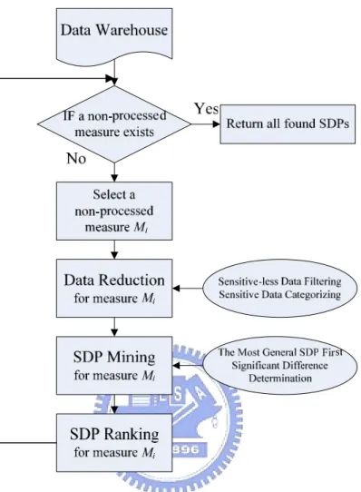
The WISDOM algorithm, as shown in Figure 4.1, is designed for discovering the possible SDPs in a given Data Warehouse efficiently. The WISDOM algorithm processes one measure at a time, and includes three steps: Data Reduction step, SDP Mining step, and SDP Ranking step. First, Data Reduction step reduces the data size by filtering the sensitive-less and categorizing the continuous data into discrete data. Next, SDP Mining step finds the possible SDPs from the reduced Data Warehouse by a tree-like greedy algorithm. Finally, SDP Ranking step sorts the found SDPs from more important to less important.

Figure 4.1: The flowchart of WISDOM algorithm

The pseudo code of WISDOM algorithm is listed in Table 4.1.

Table 4.1: The WISDOM algorithm

WISDOM(DW, α, β, γ, Depth)

Input:

DW: A data warehouse; α: A confidence level;

β: A sensitivity ratio threshold;

Depth: A search depth threshold; Output:

SDPs: The SDPs;

Begin

Set SDPs ← ψ;

For each Mi of Measure, Do

DW’ ← DataReduction(DW, Mi, β);

Set SDPs’ ← ψ;

SDPMining(DW’, Mi, Dim, ψ, α, γ, ψ, Depth, SDPs’);

SDPs ← SDPs ∪ SDPRanking(SDPs’); Return SDPs;

End

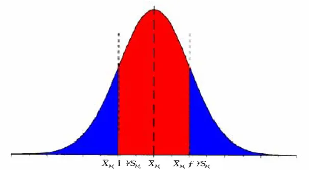
4.1. Data Reduction step

Without loss of generality, the values of measure Mi are distributed in normal

distribution as shown in Figure 4.2. Lots of records are distributed nearly the mean,

i

M

X , but these records are sensitive-less about measure Mi. When the size of records

is huge, processing these sensitive-less records will become very inefficient. Therefore, the Sensitive-less Data Filtering heuristic is proposed to filter these sensitive-less records. In addition, computing the continuous measure also consumes a lot of computational power; thus, Sensitive Data Categorizing heuristic is proposed to categorize the continuous measure into discrete measure further.

i M X i i M M S X +β i i M M S X −β

Figure 4.2: The normal distribution

HEURISTIC 1: Sensitive-less Data Filtering

The Sensitive-less Data Filtering heuristic filters the sensitive-less records about measure Mi between XM_i +βSM_i and XM_i −βSM_i, where XM_i and SM_i are the mean and standard deviation of measure Mi, and β is sensitivity ratio threshold. The

value of β can be greater than or equal to 0 to infinity. The smaller β will filter

fewer records and own better accuracy and, on the other hand, the bigger β will

filter more records and own worse accuracy.

■

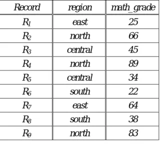
EXAMPLE 3:

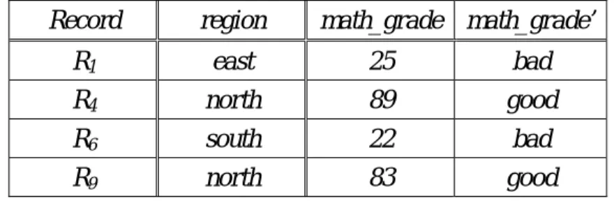
Based on EXAMPLE 1, Table 4.2 shows the records with one attribute, region, and one measure, math_grade.

Table 4.2: The records with attribute region and measure math_grade Record region math_grade

R1 east 25 R2 north 66 R3 central 45 R4 north 89 R5 central 34 R6 south 22 R7 east 64 R8 south 38 R9 north 83

In Table 4.2, X_{math_grade} is 51.78, and S_{math_grade} is 24.67. Given β = 1,

grade math grade

math S

X _{_} +β _{_} is 76.45, and X_{math_grade}−βS_{math_grade} is 27.11. After

applying Sensitive-less Data Filtering heuristic, R2, R3, R5, R7, and R8 are filtered due

to their math_grade is between Xmath_grade−βSmath_grade and Xmath_grade +βSmath_grade, and the result is shown in Table 4.3.

Table 4.3: The records after applying Sensitive-less Data Filtering heuristic Record region math_grade

R1 east 25 R2 north 66 R3 central 45 R4 north 89 R5 central 34 R6 south 22 R7 east 64 R8 south 38 R9 north 83

■

HEURISTIC 2: Sensitive Data Categorizing

The Sensitive Data Categorizing heuristic categorizes the origin continuous

measure Mi into a new discrete measure Mi’ = {good, bad}. The records whose

measure Mi is greater than XM_i +βSM_i are labeled as good. On the contrary, the records whose measure Mi is less than XM_i −βSM_i are labeled as bad.

■

EXAMPLE 4:

Following the EXAMPLE 3, a new Measure math_grade’ is added, as shown in

Table 4.4. R4 and R9 are labeled as good due to their math_grade is greater than

i i M

M S

X +β , and R1 and R6 are labeled as bad due to their math_grade is less than

i i M

M S

X −β .

Table 4.4. The records after applying Sensitive Data Categorizing heuristic Record region math_grade math_grade’

R1 east 25 bad

R4 north 89 good

R6 south 22 bad

R9 north 83 good

Although the Sensitive-less Data Filtering and Sensitive Data Categorizing heuristics can reduce the data size to decrease the process time, it will loss some accuracy contrarily. These heuristics are proposed based on our experiences and discussing with senior researchers, so they are just one of the reducing data size methods.

Data Reduction step uses the Sensitive-less Data Filtering and Sensitive Data Categorizing heuristics to reduce the data size. The pseudo code of DataReduction

algorithm is listed in Table 4.5.

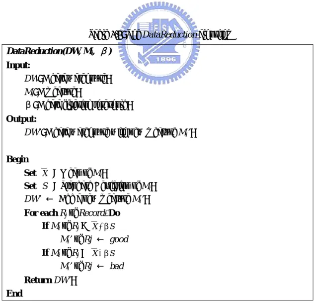
Table 4.5: The DataReduction algorithm

DataReduction(DW, Mi, β)

Input:

DW: A data warehouse; Mi: A measure;

β: A data filtering threshold; Output:

DW’: A data warehouse with new measure Mi’;

Begin

Set X = Mean of Mi;

Set S = Standard Deviation of Mi;

DW’ ← Add a new measure Mi’;

For each Rj of Record, Do

If Mi of Rj > X β+ S Mi’ of Rj ← good If Mi of Rj < X β− S Mi’ of Rj ← bad Return DW’; End

4.2. SDP Mining step

Data Reduction step filters the sensitive-less records and categorizes the

continuous measure Mi to a new discrete measure Mi’. For the original continuous

measure Mi, researches find significant differences by using statistical testing;

however, how can we find the SDPs from the new discrete measure Mi’? Therefore, a

definition, Score and Range, and Significant Difference Determination heuristic are proposed as follows. The Score and Range definition is used to calculate the difference among different attribute values of an attribute, and the Significant Difference Determination heuristic is used to determine whether the difference is

significant or not.

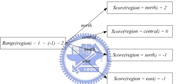
DEFINITION 4: Score and Range

Given an attribute Aij = {Vijk| k = 1…g(i, j)} and a discrete measure Mi’. GA_ij=V_ijk is the number of records whose attribute Aij = Vijk and measure Mi’ = good, and

ijk ij V

A

B ₌ is the number of records whose attribute Aij = Vijk and measure Mi’ = bad.

Score(Aij = Vijk) can be used to represent the relation between the total mean XM_i and the mean

ijk ij V

A

(

)

     ≠ + + − = = = = = = = = otherwise B G if B G B G V A

Score ij ijk ij ijk

ijk ij ijk ij ijk ij ijk ij V A V A V A V A V A V A ijk ij 0, 0 , (4.1)

The value of Score(Aij = Vijk) is between 1, representing all the values of measure

Mi’ are good, and -1, representing all the values of measure Mi’ are bad.

Range(Aij) is the maximum difference of {Score(Aij = Vijk)| k = 1,2,…,g(i, j)}, and

it can be used to represent the difference in the attribute Aij. Range(Aij) is defined as:

( )

A

{

Score

(

A V

)

k g

( )

i j

}

{

Score

(

A V

)

k g

( )

i j

}

Range _ij =max _ij = _ijk | =1,2,_K, , −min _ij = _ijk | =1,2,_K, ,

(4.2)

Due to the value of Score(Aij = Vijk) is between 1 and -1, the value of Range(Aij)

is between 2 and 0.

■

The idea of Score(Aij = Vijk) is from the z-score of the mean XA_ij=V_ijk . The value

good means this record’s measure Mi is greater than XM_i +βSM_i, and the value bad means this record’s measure Mi is less than XM_i −βSM_i. Hence, XA_ij=V_ijk can be calculated as:

(

)

(

)

i ijk ij ijk ij ijk ij ijk ij i ijk ij ijk ij ijk ij i i ijk ij i i ijk ij M V A V A V A V A M V A V A V A M M V A M M V A S B G B G X B G B S X G S X X β β β = = = = = = = = = ₊ − + = + − + + = The z-score of ijk ij V A

X ₌ , Score(Aij = Vijk), can be calculated as:

(

)

ijk ij ijk ij ijk ij ijk ij i i ijk ij V A V A V A V A M M V A ijk ij B G B G S X X V A Score = = = = = + − = − = = β

Hence, Score(Aij = Vijk) can be used to represent the z-score of the mean

ijk ij V

A X ₌ .

EXAMPLE 5:

Given the attribute region and measure math_grade’ shown in Table 4.4, the Scores and Range are calculated as:

Score(region = north) = 0 2 0 2 + − = 1 Score(region = central) = 0 Score(region = south) = 1 0 1 0 + − = -1

Score(region = east) = 1 0 1 0 + − = -1

Range(region) = Score(region = north) - Score(region = south) = 1 – (-1) = 2

The Score and Range can be represented as Figure 4.3.

Figure 4.3: The Score and Range of attribute region

■

Range(Aij) can be used to represent the difference of means of different attribute

values in an attribute Aij. Obviously, the bigger Range(Aij) represents there is more

significant difference in different attribute values in attribute Aij. Hence, the

Significant Difference Determination heuristic is proposed to determine whether there

HEURISTIC 3: Significant Difference Determination

Given an attribute Aij = {Vijk| k = 1,2,…g(i, j)}, and a measure Mk’, if Range(Aij)

is greater than or equal to γ , there exist a SDP, (Aij) : Mk, where γ is significance

determination threshold.

■

EXAMPLE 6:

Given the attribute region and measure math_grade’ shown in Table 4.4, the Range(region) = 2 has been calculated in EXAMPLE 5. Given γ = 0.4,

Range(region) ≥ γ = 0.4

Hence, there exists the SDP

(region) : math_grade (4.3)

■

In general, researchers are interested in investigating the more general human behavior and social phenomenon. If there is a significant difference on the more general phenomenon, they won’t usually be interested in the more specific one. Hence, The Most General SDP First heuristic is proposed.

HEURISTIC 4: The Most General SDP First

The Most General SDP First heuristic is that the general SDP is more interesting

than the specific SDP. The “general” means the higher level SDP and fewer dimensions SDP is better. Hence,

z Higher-level SDP is more interesting than lower-level SDP.

z Fewer-dimension SDP is more interesting than more-dimension SDP. ■

The following two examples explain The Most General SDP First heuristic more clearly.

EXAMPLE 7:

Given two SDPs:

(region) : math_grade (4.4)

(city) : math_grade (4.5)

If there is a significant difference between different resident regions on measure math_grade, researchers won’t usually be interested in whether there is a significant

difference between different resident cities on measure math_grade or not.

EXAMPLE 8:

Given two SDPs:

(gender) : math_grade (4.6)

(gender | city = Taipei) : math_grade (4.7)

If there is a significant difference between different gender on measure math_grade, researchers won’t usually be interested in whether there is a significant

difference between different gender in measure math_grade for the records only living in Taipei or not.

■

The Most General SDP First heuristic is proposed based on our experiments and

discussing with senior researchers. It’s just a general phenomenon when researchers find the significant difference. In other words, it will not always be correct at different situations. For example, researchers might also be interested in whether there is a significant difference between different gender on measure math_grade for the records only living in Taipei in EXAMPLE 8. However, the complexity of the SDPD problem can be decreased effectively by using The Most General SDP First heuristic.

Based on the Significant Difference Determination and The Most General SDP First heuristics, SDPMining algorithm is a greedy algorithm, and it searches the Data

Warehouse to find the SDPs like a BFS search tree. The pseudo code of SDPMining

Table 4.6: The SDPMining algorithm

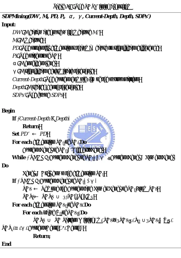
SDPMining(DW’, Mi, PD, Pi, α, γ, Current-Depth, Depth, SDPs’)

Input:

DW’: A data warehouse with measure Mi’;

Mi: A measure;

PD: The potential dimensions that may cause to significant difference; Pi: The parents of PD;

α: A confident level;

γ: A significant determinate threshold;

Current-Depth: The current complexity of the output pattern; Depth: A search depth threshold;

SDPs’: The found SDPs;

Begin

If (Current-Depth > Depth) Return;

Set PD’ ← PD;

For each dimension PDi of PD, Do

Current Level of PDi = Highest–Level;

While ( RANGE(Current Level of PDi) <γ || Current Level = Lowest Level) Do

Levelt = Drill down the dimension PDi; If ( RANGE(Current Level of PDi) ≥γ)

PD’ ← Remove the Current and Lower Level of PDi From PD’;

SDP’← SDP’ ∪ {(PDi| Pi ):m}; For each dimension PD’ i of PD’, Do

For each value Vi of PD’ i, Do

SDP’ ∪ SD Pattern Mining( m, PD’ – {PD’ i}, Pi ∪{PD’ i= Vi},

SDS ,α,γ, Current-Depth+1, Depth ); Return;

End

At the beginning, it computes the Range(Ai1) of for the first attribute Ai1 of each

significant, the rest attributes of dimension Di will not be searched due to the heuristic.

All the non-significant dimensions will be expanded to the next level and search go on. The following two examples explain SDPMining algorithm more clearly.

EXAMPLE 9:

At the beginning, SDPMining algorithm computes the Range(Ai1) of for the first

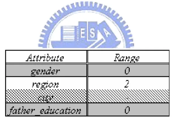
attribute, gender, region, and father_education, of each dimension. Due to the attribute region is significant, the attribute city will not be searched. The attribute region is significant and the attribute gender and father_education are not significant.

The result is shown in Figure 4.4.

Figure 4.4: The result after searching the first level in

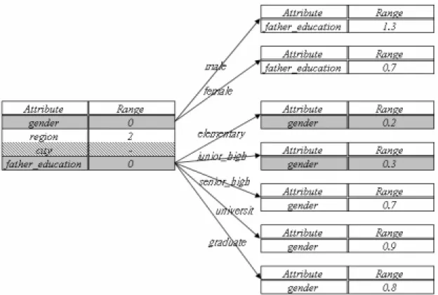
Figure 4.5: The result after searching the second level in

The following SDPs can be found by Figure 4.5: (region) : math_grade

(father_education| gender = male) : math_grade

(father_education| gender = female) : math_grade

(gender| father_education = senior_high) : math_grade

(gender| father_education = university) : math_grade

(gender| father_education = graduate) : math_grade

■

EXAMPLE 10:

attribute, gender, region, and father_education, of each dimension. Due to the attribute region is not significant, the attribute city is also processed. The attribute region is significant and the attribute region, gender and father_education are not

significant. The result is shown in Figure 4.6.

Figure 4.6: The result after searching the first level in

After expanding the non-significant attribute region, the result is shown in Figure 4.7.

Figure 4.7: The result after searching the second level in

The following SDPs can be found in Figure 4.7: (city) : math_grade

(gender| region = north) : math_grade

(father_education| region = north) : math_grade

(father_education | region = central) : math_grade

(gender | region = east) : math_grade

4.3. SDP Ranking step

SDP Ranking step sorts the SDPs in the order of importance by the Range(Aij), and the Standard Deviation of Score. Range(Aij) represents the degree of difference; hence, Range(Aij) can be used to sort the SDPs found in SDP Mining step. In addition, the Standard Deviation of Score can also be used to sort the SDPs because the bigger standard deviation expresses the wider distribution. The pseudo code of SDPRanking algorithm is listed in Table 4.7. For example, there are three patterns of Figure 4.7 as follows:

Pattern 1: (gender| region = north) : math_grade Range = 0.9

Pattern2: (father_education| region = north) : math_grade Range = 0.5

Pattern3: (father_education | region = central) : math_grade Range = 0.5

Since the range of Pattern 1 is greater than Pattern 2 and range of Pattern 2 is equal to Pattern 3, Pattern 1 is more interesting than Pattern 2 and we need observe the standard deviations. Here, the Scores distribution of Pattern 2 and Pattern 3 are denoted as Scores 2 and Scores 3, respectively.

Scores2: { Score(elementary), Score(junior_high), Score(senior_high), Score(university), Score(graduate) } = { -0.3, 0, 0, 0, 0.2 }

Scores3: { Score(elementary), Score(junior_high), Score(senior_high), Score(university), Score(graduate) } = { -0.3, -0.2, 0.1, 0.2, 0.2 }

Since standard deviations of Scores 2 and Scores 3 are 0.2 and 0.23, respectively, the Pattern 3 is more interesting than Pattern 2.

Table 4.7. The SDPRanking algorithm

SDPRanking(SDPs’)

Input:

SDPs’: The SDPs are not ranked yet; Output:

SDPs: The SDPs have already been ranked;

Begin

Set SDPs ← ψ;

SDPs ← Sorting SDPs’ by Range(Aij), Standard Deviation of Score DESC;

Return SDPs; End

Chapter 5. Experiment

In this chapter, we design the experiments to evaluate the accuracy and the execution time of the WISDOM. Firstly, we simply explain our design of the experiments. Secondly, we experiment on the accuracy of the WISDOM with parameter γ and β in Section 5.1. Finally, we discuss the issue of the execution time about parameter β, dimensions and concept hierarchy in Section 0.

As shown in Figure 5.1, a digital divide data warehouse (數位落差問卷資料庫) having six questionnaire datacube, executive (行政問卷結果), senior high school(高 中問卷結果), vocational school(高職問卷結果), elementary school (國小問卷系統), junior high school (國中問卷系統) and teacher (教師問卷系統) is used in this thesis, and its data source is a survey of the Assessment and Analysis of Establishing the

Digital Divide Criteria Indexes and Evaluation for Current K-12 Digital Divide Status in School (A project of the Ministry of Education, ROC) [24] [25]. In our

experiments, the elementary school questionnaire datacube using the star schema is chosen as shown in Figure 5.2.

The elementary school datacube has lots of measures and several dimensions with concept hierarchical structure. For example, the datacube has dimensions like gender (the gender of the students), location (the location which the student lived, and the location has dimension area, city), father education (the education level of the student’s father), mother education (the education level of the student’s mother), etc., and measure like Q11 (你會上網找資料嗎), Q12 (你會和其他同學透過網路合作， 收集資料完成作業嗎？), Q13 (你會上網路跟朋友或同學討論問題嗎？), etc., and the measure SUM11_16 is the sum of the measures Q11, Q12, Q13…and Q16. SUM11_16 implies the quota of well-fine using the computer resource. In order to

simplify our discussion, we select 3,504 records from the elementary school datacube and call it DB3504. The elementary school datacube has 67,463 records. The following experiments are done on the DB3504.

Figure 5.2 The star schema of the elementary school data cube (國小問卷結果) of digital divide data warehouse

5.1. Accuracy and Recall of the WISDOM

In this section, we explain experiments briefly and show the results of the accuracy and recall of parameter γ and β. Without loss of the generality, we assume the value of confident level 1-α is 95%, and the value of α is 0.05.

The accuracy means the probability of the SD pattern found by WISDOM is real significant in the statistic test, and the recall means the percentage of the total SD patterns which WISDOM found. For example, there are 10 SD patterns found by WISDOM and only 7 SD patterns are real significant in the statistical test, and the

number of real SD pattern is 14. Hence, the accuracy and recall are 70 % and 50%, respectively.

In order to evaluate the accuracy, we use the statistic tool – SPSS to test and find the entire significant difference pattern amount these dimensions versus the measure SUM11_16 followed the heuristics of the WISDOM. The chosen dimensions and results of SPSS are shown in Figure 5.3. Hence, we can evaluate the accuracy of the WISDOM by this pattern found manually in the SPSS process.

Dimension

Is significant

difference

buddy_level3 Ｏ computer_stuent_level3 Ｏ buddy_ie_level3 Ｏ internetTime Ｏ computer_teacher_level3 Ｏ motherEdu Ｏ fatherEdu Ｏ citytype Ｏ teacher_communication Ｏ buddy_level2 Ｏ parents Ｘ buddy_ie_level2 Ｘ computer_stuent_level2 Ｏ L_region Ｏ motherIE Ｏ fatherIE Ｏ computer_teacher_level2 Ｘ gender Ｘ seed Ｘ

5.1.1 Parameter γ versus Accuracy and Recall

In previous section, we have found several significant difference pattern using a manually method. In this section, we evaluate the accuracy and recall of WISDOM by comparing the results of WISDOM and the results of SPSS. Firstly, we assume the value of the parameter β is zero. We will discuss the value of β in next section. Secondly, in order to simplify the discussion of the SPSS process, we assume the value of the parameter depth is 1. Then several experiments are done with accuracy and recall to evaluate the parameter γ. The value of parameter γ ranges from 0.1 to 2 increasing by 0.1. The results of accuracy and recall are shown in Figure 5.4.

0.00% 20.00% 40.00% 60.00% 80.00% 100.00% 120.00% 0.1 0.3 0.5 0.7 0.9 1.1 1.3 1.5 1.7 1.9 γ accuracy recall

Figure 5.4 The accuracy and recall of WISDOM. γ=0.1~2 increasing by 0.1 β=0, depth=1

In Figure 5.4, we can find that the accuracy intersect recall in the section (0.1~0.3) of γ. Hence, some experiments are done with accuracy and recall to evaluate the parameter γ. The value of parameter γ ranges from 0.1 to 0.3

increasing by 0.01. The results of accuracy and recall are shown in Figure 5.5

In Figure 5.5, we can find that the recall will almost be 100% when the γ is small than 0.16. When the γ is 0.16, the accuracy of WISDOM is 87.5%. In addition, if the gamma is greater than 0.25 the accuracy will almost be 100% but the recall will decrease seriously. Hence the value of the parameter γ which we suggested is 0.16 because it has the higher accuracy 87.5% and the ideal recall 100.

0.00% 20.00% 40.00% 60.00% 80.00% 100.00% 120.00% 0.1 _{0.12 0.14 0.1}6 _0.18 0.2 _{0.22 0.24 0.26 0.28} 0.3 γ accuracy recall

5.1.2 Parameter β versus Accuracy and Recall

We have got the best value of parameter γ in Section 5.1.1. In this section, we will discuss the relationship of the parameter β versus accuracy.

Firstly, we assume the value of parameter γ is 0.16, and then some experiments are done with the accuracy and recall to evaluate the parameter β. The value of β is from 0 to 2 increasing by 0.1. The results are show in Figure 5.6. we can find the recall is decreasing seriously when the value of β is greater than 1.9. Hence the value of the parameterβwhich we suggested is not greater than 1.9 and we will discuss the relationship between parameter β and execution time in next section. 0.00% 20.00% 40.00% 60.00% 80.00% 100.00% 0 0.2 0.4 0.6 0.8 1 1.2 1.4 1.6 1.8 2 β accuracy recall

5.2. Performance of the WISDOM

We have already known relationship between accuracy and recall versus the value of parameter β and γ . In this section, we show the results of the performance, execution time, of WISDOM in different value of parameter β and depth, number of dimensions and number of concept hierarchies.

5.2.1 Parameter β versus Execution Time

Firstly, we evaluate the execution time of the WISDOM. The value of β is from 0 to 2 increasing by 0.1. The results are shown in Figure 5.7. After observing Figure 5.7, we can find the trend of the execution time of WISDOM is decreasing when the beta is growing up.

2,400 2,500 2,600 2,700 2,800 2,900 3,000 0 0.2 0.4 0.6 0.8 1 1.2 1.4 1.6 1.8 2 β ms execution time

Figure 5.7 The execution time of WISDOM γ=0.16,depth=1,β=0~2 increasing by 0.1

Secondly, we compare the accuracy which mentioned in the Figure 5.6 of the front section and the execution time of the WISDOM mentioned in Figure 5.7. In

Figure 5.8, the results show that the execution time decreases about 10% when the β is greater than 1.4 and the accuracy keeps at least 80%. Hence we suggest the value of parameter β is 1.4. 0.00% 20.00% 40.00% 60.00% 80.00% 100.00% 120.00% 0 0.2 0.4 0.6 0.8 1 1.2 1.4 1.6 1.8 2 β

accuracy exectuion time

Figure 5.8 The accuracy and execution time of WISDOM.γ=0.16, depth=1,β=0~2 increasing by 0.1

5.2.2 Depth versus Execution Time

In this section, several experiments are done with the execution time to evaluate the parameter depth. We assume the value of parameter γ is 3 and fix β is 0. The results are shown in Figure 5.9.

In this experiment, we prefer to discuss the relationship without some heuristics of WISDOM. Since the maximum range is 2 and we assume the value of parameter γ is 3, we can guarantee the case is the worst case of execution time without performing some heuristics. For example, the heuristic 4, “The Most General SDP

First”, will prune lots of search space and save much execution time. We can

section. The execution time using heuristic 4 is 2,922ms (The DB3504 has more than 12 dimensions), and the execution without heuristic1 is longer than 250,000ms. And in Figure 5.8, we can find that the value of parameter β also affects the execution time deeply.

In Figure 5.9, the execution time is growing up in an exponential trend. Hence, we suggest the value of the parameter depth is smaller than 3.

0 2,000,000 4,000,000 6,000,000 8,000,000 1 2 3 4 5 Depth ms time

Figure 5.9 The execution time of WISDOM. γ=3, depth=1~5 increasing by 1,β=0.

5.2.3 Dimensions versus Execution Time

Several experiments are done with the execution time to evaluate the number of dimensions. The number of dimensions ranges form 3 to 12, the value of parameter β is 0 and the value of parameter γ is 3 as described in section 5.2.2. In Figure 5.10, we can observe that the execution time of WIDSOM almost linearly growing with number of dimensions.

0 50,000 100,000 150,000 200,000 250,000 300,000 3 4 5 6 7 8 9 10 11 12 dims ms execution time

Figure 5.10 The relationship between number of dimensions and execution time.γ=3, depth=3,β=0.

5.2.4 Concept Hierarchy versus Execution Time

We have known the relationship of dimensions and execution time which is almost growing linearly. In this section, some experiments are done with the execution time to evaluate the number of level per dimension. We done the experiments as follows.

Firstly, we also assume the value of parameter γ is 3 ,β is 0 and the depth is 3 as described in section 5.2.2. And the number of dimension ranges from 3 to 7 and increasing by 1.. We discussion the WISDOM on three cases, each case has k-levels per dimension. The value of k ranges from 1 to 3 and increasing by 1. In Figure 5.11, we can observe that the execution time of WISDOM increases rapidly when the concept hierarchy gets more complex.

0 200,000 400,000 600,000 800,000 1,000,000 3 4 5 6 7 dims ms

1 level per dim 2 level per dim 3 level per dim

Figure 5.11 The relationship between concept hierarchy and execution time. γ=3, depth=3,β=0.

5.3. Experiments Summary

We applied the WISDOM to the digital divide data warehouse and we found some interesting patterns. For example, the pattern, “(computer_teacher_level2|seed='資訊種子學校'):SUM11_16”, implies these is a significant difference between different groups of computer teacher level 2 in the computer seed school, and the researchers are unaware this pattern.

Chapter 6. Conclusion

In the questionnaire analysis, finding whether there is a significant difference between two or more groups in one measure is one of the major problems which social science researchers are concerned about. However, finding possible significant differences is difficult for social science researchers. We call it Significant Difference Unawareness issue. In order to overcome the Significant Difference Unawareness issue, in this thesis, we firstly build a data warehouse by integrating the questionnaire data and secondary data. Secondly, the WISDOM algorithm is proposed to find the possible significant differences from the data warehouse semi-automatically.

The results of experiments show that the suggested value of the parameter γ is 0.16 because there is a higher accuracy 87.5% and an ideal recall 100%. The execution time decreases about 10% when the β is greater than 1.4 and the accuracy keeps at least 80%. Hence, we suggest the value of parameter β is between 0~1.4. Furthermore, several experiments are done with the execution time to evaluate dimensions and levels of concept hierarchy. The execution time is rapidly growing up when the number of dimensions or the number of levels of concept hierarchy is increasing.

In the near future, we will aim to apply the WISDOM in several domains like digital divide, statistic for business and economics. Besides, we will discuss the relationship between the value of parameter γ and the amount of records.

Furthermore, the parameter γ implies the degree of the difference. Hence, we will also discuss the relationship between degree of difference and the parameter γ in the future.

Reference

[1] Data Modeling Techniques for Data Warehousing, IBM Redbooks , IBM

Corporation, U.S.A., 1998.

[2] S. Chaudhuri and U. Dayal, An Overview of Data Warehousing and OLAP

Technology. SIGMOD Record 26(1): pp. 65-74, 1997.

[3] G. D. Garson, Advances in Social Science and Computers: A research annual,

H61.3 A 38 v.1, 1989.

[4] M. Golfarelli and S. Rizzi, Designing the Datawarehouse： Key Steps and

Crucial Issues, Journal of Computer Science and Information Management, vol. 2, n.3, 1999.

[5] H. Gupta and I. S. Mumick, Selection of Views to Materialize in a Data

Warehouse, IEEE Alencia, Spain, 1998.

[6] J. Han and M. Kamber, Data Mining: Concepts and Techniques, London, 2001.

[7] W. H. Inmon, Building the Operational Data Store, John Wiley & Sons Inc.,

1996.

[8] R. Kimball, The Data Warehouse Toolkit, John Wiley & Sons Inc., 1996.

[9] R. Kimball and L. Reeves, The Data Warehouse Lifecycle Toolkit, Wiley

Computer Publishing, 1998.

[10] M. Kortnik and D. Moody, From Entities to Stars, Snowflakes, Clusters,

Constellations and Galaxies: A Methodology for Data Warehouse Design. In proceeding of the 18th International Conference on Conceptual Modelling. Industrial Track, 1999.

[11] J. J. McGill, Statistics for Business & Economics, 7/e, 2006.

[12] R. Páircéir and S. McClean, Discovery of Multi-level Rules and Exceptions

[13] T. Palpanas and N. Koudas, Using Datacube Aggregates for Approximate Querying and Deviation Detection, IEEE KDE Trans., 2005.

[14] L. Rokach and O. Mainmon, Top-down Induction of Decision Trees Classifiers -

a Survey, IEEE Transaction on Systems, Man, and Cybernetics, 2005.

[15] S. Russell and P. Norvig, Artificial Intelligence：A Modern Approach, 2/e, 2005.

[16] T. L. Saaty, The Analysis Hierarchy Process, New York, 1980.

[17] S. Sarawagi, Discovery-Driven exploration of OLAP datacubes, In Proceedings

of International Conference on Extending Database Technology, pp.168-182, 1998.

[18] S. Sarawagi, User-Adaptive Exploration of Multidimensional, In Proceedings of

the 26th VLDB Conference, Cairo, Egypt, 2000.

[19] A. Shoshani, OLAP and Statistical Databases Similarities and Differences,

PODS Tucson Arizona USA, 1997.

[20] H. Zhang and B. Padmanabhan, Research track papers On the Discovery of

Significant Statistical Quantitative Rules, ACM KDD Trans., 2004.

[21] 尹相志，SQL2000 Analysis Service 資料採礦服務，維科圖書有限公司，民 國91 年。 [22] 林傑斌等，資料採掘與 OLAP 理論與實務，文魁資訊股份有限公司，民國 91 年。 [23] 邱皓政，量化研究法（二）：統計原理與分析技術，雙葉書廊，民國94 年。 [24] 曾憲雄，張維安，黃國禎，建立中小學數位學習指標暨城鄉數位落差之現 況調查、評估與形成因素分析報告，教育部數位學習國家型計劃，民國 93 年。 [25] 曾憲雄，張維安，黃國禎，建立中小學數位學習指標暨城鄉數位落差之現 況調查、評估與形成因素分析報告，教育部數位學習國家型計劃，民國 94 年。