都會擷取環形光網路之低運算複雜度動態訊務彙集機制

全文

(1)國立交通大學. 電信工程學系碩士班. 碩士論文. 都會擷取環形光網路之低運算複雜度動態訊務彙集機制. Computation-Efficient Algorithms for Dynamic Traffic Grooming in Metro-Access Ring Network. 研究生︰郭朕逢指導教授︰張仲儒教授. 中華民國九十四年六月. i.

(2) 都會擷取環形光網路之低運算複雜度動態訊務彙集機制. Computation-Efficient Algorithms for Dynamic Traffic Grooming in Metro-Access Ring Network 研究生︰郭朕逢指導教授︰張仲儒. Student: Chen-Fong Kuo Advisor: Dr. Chung-Ju Chang. 教授. 國立交通大學電信工程學系碩士班碩士論文. A Thesis Submitted to Institute of Communication Engineering College of Electrical Engineering and Computer Science National Chiao Tung University in Partial Fulfillment of the Requirements for the Degree of Master of Science in Electrical Engineering June 2004 Hsinchu, Taiwan, Republic of China. 中華民國九十四年六月 ii.

(3) 都會擷取環形光網路之低運算複雜度動態訊務彙集機制研究生︰郭朕逢. 指導教授︰張仲儒教授. 國立交通大學電信工程學系碩士班中文摘要在近幾年裡，同步光纖(SONET)環狀網路被大幅應用在光纖基礎建設上。而且隨著時間經過，光纖網路的發展已經有了很大的進步，不只如此訊務的流量也大幅激增。此外由於分波多工(WDM)的技術的成熟並且被大幅應用下，光纖網路的傳輸容量大幅的提升。然而相對於一個波長提供的頻寬，訊務的流量仍是相當的小。所以為了有效的利用資源，可以利用訊務彙集的技術，把需求頻寬小的訊務彙集到頻寬大的波長上。在本篇論文中，我們考慮動態訊務彙集的問題。而且我們的目標是讓波長頻寬的使用率達到最高，同時降低新連線呼叫拒絕率。根據要達成的目標，我們把這個問題公式化成整數線性規劃(ILP)的問題，並且為了解這個問題，我們從模擬退火演算法的精神，提出一個 STGA 演算法來求的最佳解。但是因為計算複雜度的關係，我們另外提出計算法雜度較低的 HTGA 的演算法。在 HTGA 演算法裡面主要有三個步驟：訊務彙集的動作、波長指派的動作、訊務重新被安排的動作。這些動作的主要目的是在儘可能不要改變光通道的情況下讓系統的使用率更好。從模擬裡我們可以得到幾個結果，HTGA 在系統使用效率方面只比 STGA 差 10%左右，而在計算複雜度方面 HTGA 卻是比 STGA 低很多；除此之外，HTGA 在光通道被重新安排的數目也是比 STGA 少很多。從這些結果顯示，我們可以指出 HTGA 是個有可行性且吸引人的演算法。. i.

(4) Computation-Efficient Algorithms for Dynamic Traffic Grooming in Metro-Access Ring Network Student: Chen-Fong Kuo. Advisor: Dr. Chung-Ju Chang. Institute of Communication Engineering National Chiao Tung University. Abstract In recent years, synchronous optical network (SONET) ring networks have been widely deployed for the optical network infrastructure. The progresses of optical networks evolve with time; meanwhile, the carried traffic streams surge. The transmission capacity of an optical network largely increases because of the development and application of wavelength division multiplexing (WDM) technologies. However the required bandwidth of a traffic stream is also much smaller than the bandwidth capacity of a wavelength. Thus, in order to efficiently utilize the network resources, many lower-speed traffic streams can be multiplexed onto a high-speed wavelength by traffic-grooming technique. In the thesis, we consider the traffic grooming problem, which the property of the traffic is dynamic and nonuniform traffic. Our objective is to effectively reduce the new call blocking rate and maximize the utilization efficiency of the wavelengths which are used by the system. Integer linear problem (ILP) methodology is applied to formulate for this problem. And, in order to solve the ILP, we first propose a simulated annealing-based traffic grooming (STGA) algorithm to obtain the optimal solution. However, the STGA algorithm is infeasible due to its computation complexity. Alternatively, we propose a heuristic algorithm, called a heuristic-based traffic grooming (HTGA) algorithm. There are the three main operations in HTGA algorithm: operation of traffic grooming, ii.

(5) operation of wavelength assignments, operation of traffic rearrangement. The main purpose of these operations is to achieve the better system utilization without changing the lightpath topology as could as possible. From the simulation evaluation, network performance measures are observed. For system utilization, the HTGA algorithm is only 10% less than the STGA algorithm, whereas the computation complexity of the STGA algorithm is much larger than that of the HTGA algorithm. In addition, the number of rearranged lightpaths by the HTGA algorithm is fewer than the ones by the STGA algorithm. From these results, we can conclude that the HTGA algorithm is a feasible and attractive algorithm.. iii.

(6) 誌. 謝. 經過了兩年的碩士生涯的洗禮和努力，碩士論文終於順利的完成，但這並不是我自己一個人辦到的，我必須要感謝許許多多幫助過我的貴人。首先必須感謝恩師張仲儒教授的殷勤指導、批評指正以及無數的金玉良言。再來感謝學長陳義昇博士除了讓我學到嚴謹的治學態度與研究方法，老師和義昇學長更開啟了一扇“超越自我”的大門，砥礪我們時時刻刻不忘充實自己，使自己能禁得起時代的考驗。在實驗室的其他學長們，我要先感謝立峯學長，沒有學長在百忙之中犧牲自己的時間並熱心參與討論、傾囊相授，學弟的研究過程中勢必將困難許多；再來要感謝聰明絕頂、妙語如珠的家慶、正文、芳慶、詠翰、界和、文祥學長和青毓學姊，總是在我最需要幫助的時候給予我許多寶貴的經驗及建議；另外還要感謝崇楨、皓堂、俊憲與同浩學長在我剛進實驗室時親切的給予提攜與照顧，讓我能很快的適應研究生的生活。除了學長們的提攜、照顧之恩，還有要感謝我的同學們志明、立忠、凱元和宗軒陪我一同走過這一段日子；並且琴雅、煖玉、俊帆、家源和 JＢ榮巴提學弟妹們對我的幫助也是功不可沒，感謝你們替我分擔許多壓力並與我分享生活點滴。最後，我要感謝我的父母及家人，在我遇到挫折時給我幫助及照顧，你們的的支持是讓我勇往直前的最大的動力，並且讓我能專心於論文的研究。我願將這碩士論文獻給所有幫助過我、愛護我的人，希望你們與我一起分享這得來不易的成果及心中的喜悅。郭朕逢謹誌民國九十四年. iv.

(7) Contents 中文摘要 ...............................................................................................................................i Abstract ...............................................................................................................................ii Acknowledgement ..............................................................................................................iv Contents...............................................................................................................................v List of Figures.....................................................................................................................vi List of Tables .....................................................................................................................vii Chapter 1 Introduction .......................................................................................................1 Chapter 2 Dynamic Traffic Grooming and Wavelength Assignment in Metro Access Ring Network ......................................................................................................................6 2.1 Network Architecture...............................................................................................6 2.2 Node Function/Capability and Operations................................................................7 2.3 Source Model ..........................................................................................................9 2.4 Problem Formulation for Traffic Grooming ...........................................................10 2.4.1 Connection request, light path, fiber link, and the related notations .............10 2.4.2 Generalized Problem Formulation...............................................................13 Chapter 3 Optimal and Suboptimal Solutions to the Dynamic Traffic Grooming Problem ...........................................................................................................................................15 3.1 Simulated Annealing-based Traffic Grooming Algorithm (STGA) .........................15 3.1.1 The Concept and Procedure of SA...............................................................16 3.1.2 The Flowchart of STGA..............................................................................18 3.2 Heuristic-based Traffic Grooming Algorithm (HTGA)...........................................20 3.2.1 Block Functionality.....................................................................................22 3.2.2 The Procedure.............................................................................................23 Chapter 4 Performance Evaluation of the Proposed Algorithms....................................31 4.1 Simulation Parameters ...........................................................................................32 4.2 Simulation Results and Discussions .......................................................................33 4.2.1 Performance Evaluation in Fixed Network Configuration............................33 4.2.2 Performance Evaluation in Various Network Configurations .......................37 Chapter 5 Conclusion........................................................................................................42 Bibliography......................................................................................................................44 Vita.....................................................................................................................................46. v.

(8) List of Figures Figure 1. Metro-Access Ring.................................................................................................7 Figure 2. Node Architecture ..................................................................................................8 Figure 3. Illustrative example of a fiber link, a lightpath and a connection request............... 11 Figure 4. Flowchart of the Simulated Annealing-based Traffic Grooming algorithm............20 Figure 5. The block diagram of HTGA algorithm ................................................................24 Figure 6. Flowchart of the HTGA algorithm........................................................................30 Figure 7. The utilization efficiency of the used wavelengths in two algorithms....................34 Figure 8. The blocking ratio in two algorithms ....................................................................35 Figure 9. Number of rearranged lightpaths per call in two algorithms ..................................35 Figure 10. The utilization efficiency of the used wavelengths in Scenario 1 ........................38 Figure 11. The blocking ratio in the Scenario 1...................................................................38 Figure 12. The utilization efficiency of the used wavelengths in Scenario 2 ........................39 Figure 13. The blocking ratio in the Scenario 2...................................................................40 Figure 14. The utilization efficiency of the used wavelengths in Scenario 3 ........................41 Figure 15. The blocking ratio in the Scenario 3...................................................................41. vi.

(9) List of Tables Table 2.1: The notations of mathematical formulation ......................................................... 11 Table 2.2: The sets of mathematical formulation..................................................................12 Table 2.3: The variables used in mathematical formulation..................................................13 Table 4.1: The parameters used in the simulation.................................................................32 Table 4.2: The value of the parameters used in the simulation..............................................33 Table 4.3: The value of the parameters used in STGA algorithm..........................................33. vii.

(10) Chapter 1 Introduction. Chapter 1 Introduction. I. n recent years, synchronous optical network (SONET) ring networks have been widely deployed for the optical network infrastructure. The progresses of optical. networks evolve with time; meanwhile, the carried traffic streams surge. The transmission capacity of an optical network largely increases because of the development and application of wavelength division multiplexing (WDM) technologies which allow multiple wavelengths to be delivered in a single fiber at the same time [1]. Besides, the capacity of one wavelength has grown up to optical-carrier (OC) 192, approximately 10 Gb/s. A traffic stream is normally assigned in one wavelength. However, the required bandwidth of a traffic stream, called lower-speed traffic stream, is much smaller than the bandwidth capacity of a wavelength. If every lower-speed traffic stream occupies an individual wavelength, bandwidth waste is an obvious and serious drawback. In order to efficiently utilize the network resources, many lower-speed traffic streams can be multiplexed onto a high-speed wavelength by traffic-grooming technique. This technique is performed by Add/Drop Multiplexer (ADM) equipment.. An overview of the. traffic-grooming technique and survey of some typical works were reported in [2]. In the design of traffic-grooming, three issues to be considered: network configuration, traffic characteristics, and cost function. For the network configuration issue, ring network architectures were mostly studied for grooming [4], [6], [7], [8], [9], [10], [12], [13], which may be long-haul backbone networks or metro networks. The ring network can also be a unidirectional ring or bidirectional ring. In addition, many researches [3], [11] also focus on 1.

(11) the mesh network, which their backbone is a long-haul backbone network. In the early stage of optical network, the ring network is employed in a long-haul backbone network. With the increasing of the traffic load, the mesh network has been studied by many researches because the mesh network sustains more traffic load than the ring network. However, for metro networks, ring network is preferable because the mesh network is an over-provisioning and expensive solution. Instead, many people study the ring network for the metro networks. For the traffic characteristics, two properties are used to describe the behavior of traffics in this thesis. One is bandwidth request and the other one is connection pattern. Traffics may be categorized into uniform or non-uniform ones according to their required bandwidth. The bandwidth request is the same for all the users, called uniform traffic; otherwise, it is non-uniform traffic. And, the traffics may also be categorized into static or dynamic ones according to system connection including the amount of connection, the occupied bandwidth of all connection. The system connection does not change with time for static traffic while it does for dynamic traffic. Notably, the required bandwidth of each call request does not change during its transmission time in this thesis. Besides, many objectives were proposed for the definitions of cost functions and may be categorized into five types. The first one is minimization of the required number of Line Terminating Equipment (LTE) over all the network nodes. The second one is reduction of the cost of actual electronic processing involved in Optical-Electric-Optical (OEO) routing or minimization of the average hop counts. The third one is minimization the maximum number of lightpaths originating/terminating at a network node. The fourth one is maximization of traffic throughput of the optical network. The last one is minimization of the blocking probability of the new call request in dynamic traffic. In [3], the traffic-grooming problem was considered WDM mesh network with static and uniform traffic. The new node architecture was proposed for a WDM mesh network with traffic-grooming capacity and cost function was designed to maximize the total. 2.

(12) successfully-routed lower speed traffic. A traffic-grooming problem in WDM ring was studied in [4], where the traffic is static and non-uniform. The authors presented a framework of bounds, both upper and lower bounds, on the optimal value of the amount of traffic electrically routed. In [5], a traffic grooming problem on general topology network was studied, where the objective of cost function was minimization of the number of required wavelengths. In this work, an integer linear programming problem was formulated for traffic grooming, and a heuristic solution was proposed. In [6], the authors considered a Min-Max objective, which was desirable to minimize the cost at the node where this cost is maximum. They presented a polynomial-time traffic grooming algorithm for minimizing the maximum electronic port cost in both uni- and bi-directional ring. The ring network was considered with static and non-uniform traffic [7]. The simulated-annealing-based heuristic algorithm for the traffic grooming problem was proposed for minimization of the total cost of electronic equipment. Both nui- and bi-directional ring were considered in [8]. It considered two kinds of traffic. One was static and uniform traffic and the other was static and non-uniform traffic. For minimizing number of wavelengths, the greedy heuristic algorithm was employed for two kinds of traffic. The author also proposed another heuristic algorithm for static and non-uniform traffic according to the same objective. In [9], the ring network was considered with static and uniform traffic. The author proposed the heuristic algorithm for minimizing number of wavelengths and also considered computational complexity. The network architecture of [10] was ring network and two kinds of traffic are considered: static and uniform traffic, static and non-uniform traffic. The heuristic algorithm was proposed for minimizing the number of transceivers in optical networks. In [11], the mesh network was considered with static and uniform traffic. And, there were three considered objectives at the same time such as maximizing the traffic throughput, minimizing the number of transceivers, and minimizing the average hop counts. In [12], the bidirectional. 3.

(13) ring was employed under the static and uniform traffic. For minimizing the number of ADMs, the tighter lower bounder is derived. The author also proposed the heuristic algorithm. Although the ring network has been studied by many researchers, dynamic and non-uniform traffic has not considered yet. Therefore, we are motivated to study the traffic grooming problem in metro-access ring network with dynamic and non-uniform traffic. In the thesis, the metro-access ring network has nodes in WDM-PON architecture connecting to end-users. We investigate the node architecture from the current equipments and propose the node architecture which is equipped in metro-access ring network and have the ability of traffic grooming. The objective of this work is to effectively reduce the new call blocking rate and maximize the utilization efficiency of the wavelength used. Integer linear problem (ILP) methodology is applied to formulate for the traffic grooming problem in this thesis. And, in order to solve the ILP, we first propose a simulated annealing-based traffic grooming algorithm (STGA) to obtain the optimal solution. However, the STGA algorithm is infeasible due to its computation complexity. Alternatively, we propose a heuristic algorithm, called a heuristic-based traffic grooming algorithm (HTGA). Although the HTGA algorithm is a suboptimal solution, the computation complexity of the HTGA is much less than that of the STGA. For our objective, we consider grooming traffic into the present lightpaths. If the new call request can not be arranged by grooming traffic, employing the unused resource is considered. Besides, in order to more effectively increase the utilization efficiency of the wavelength used, the current lightpaths are sorted in descendent order according to the value of utilization of lightpaths. Based on above, there are the three main operations in HTGA algorithm: operation of traffic grooming, operation of wavelength assignments, operation of traffic rearrangement. The operations of traffic grooming and wavelength assignments may be executed when the new call request arrives; while the operation of traffic rearrangement is executed when the required large bandwidth of a call leaves. The main purpose of these operations is to achieve the better system utilization without changing the lightpath topology 4.

(14) as could as possible. And, the blocking rate of the new call request is also reduced by HTGA algorithm. Simulation comparisons between the two algorithms were conducted in the thesis for performance evaluation. The results were demonstrated in terms of system utilization and computation complexity. In the system utilization, the HTGA algorithm is only 10% less than the STGA algorithm. And, the computation complexity of the STGA algorithm is much larger than that of the HTGA algorithm. In addition, the number of rearranged lightpaths by the HTGA algorithm is fewer than the ones by the STGA algorithm. From these results, we also point out that the STGA algorithm is infeasible with the current equipments. The thesis is organized as follows. In Chapter 2, we describe the network architecture, the node architecture. The detail of the traffic assumption is introduced in the source model of Chapter 2. In addition, the problem is mathematically formulated for the optical ring network with dynamic traffic model. In Chapter 3, the optimal STGA algorithm and suboptimal HTGA algorithm are proposed and the operations of two algorithms are described. The procedures of two algorithms are also revealed in detail in Chapter 3. The simulation results of two algorithms are discussed in chapter 4. At last, Chapter 5 concludes the thesis.. 5.

(15) Chapter 2 Dynamic Traffic Grooming and Wavelength Assignment in Metro Access Ring Network. Chapter 2 Dynamic Traffic Grooming and Wavelength Assignment in Metro Access Ring Network. T. he. basic. environment,. included. network. architecture,. and. node. architecture/function, is described in this section. Besides, the operations of the. network and source model about traffic assumption are also described here. At last, we propose the generalized problem formulation about dynamic traffic grooming and wavelength assignment in metro access ring network.. 2.1 Network Architecture As shown in Fig. 1, the network topology considered in this thesis is a WDM metro access ring architecture, consisting of of N nodes, labeled as 1, 2, …, N counterclockwise. Each node provides several PONs with tree topology to building users (BUs). The links of the network are labeled as 1, 2, …, N counterclockwise, and the link from node i to node i+1 is labeled as i., Only one fiber exists between node i and node i+1, 1 ≤ i ≤ N-1, and one fiber between node N and node 1. In addition, each fiber link contains W wavelengths, carrying traffic streams in counterclockwise directions. About the PON, we adopt one wavelength to carry traffic streams from the node to BUs and another wavelength to carry traffic streams from BUs to the node.. 6.

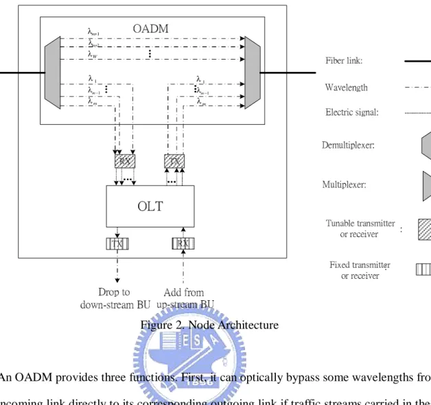
(16) Figure 1. Metro-Access Ring. 2.2 Node Function/Capability and Operations Each node in the metro access ring is equipped with an optical add-drop multiplexer (OADM), an optical line terminal (OLT), m tunable transmitter/receiver pairs, and a fixed transmitter/ receiver pair, as shown in Fig. 2. A tunable transmitter (receiver) possesses the capability of transmitting (receiving) any of W wavelengths, respectively. Conversely, a fixed transmitter and receiver possess the capability of transmitting and receiving a fixed wavelength, respectively. The tunable and fixed transmitters execute electrical-to-optical conversion, while the tunable and fixed receivers execute optical-to-electrical conversion. A multiplexer aggregates wavelengths into a single fiber while a de-multiplexer dispatches wavelengths from the fiber. Additionally, the de-multiplexer also choosees the wavelength whose traffic streams are required be dropped out of the node.. 7.

(17) λm+1 λm+2. λW λ1. λ1. λm −1 λm. λm −1. λm. Figure 2. Node Architecture. An OADM provides three functions. First, it can optically bypass some wavelengths from the incoming link directly to its corresponding outgoing link if traffic streams carried in these wavelengths are not necessary to be dropped in this node. Second, it can optically drop (terminate) some wavelengths from the incoming link to tunable receivers, and then tunable receivers convert the traffic streams carried by the dropped wavelengths into electronic form. Third, the OADM can also multiplex some wavelengths to the outgoing link. An OLT perform three functions and be operated in electrical domain. First, it can multiplex low-speed streams originating from the BUs to a high-speed stream, and then transmit the high-speed traffic stream to a tunable transmitter. Second, it can extract low-speed streams out of a high-speed stream. Third, it can transmit the low-speed traffic streams terminating at the node to the BUs by a fixed transmitter and also receive the traffic streams originating from the BUs by a fixed receiver. When the wavelengths carrying traffic streams come across the node, the node will perform one of the following operational 8.

(18) procedures, depending on the transmission conditions. 1.. If the node is the destination of the traffic streams, OADM drops wavelengths to a tunable receiver; the tunable receiver transforms data streams from the optical domain into electrical domain and sends them to an OLT; the OLT extracts the traffic streams from the high-speed traffic streams and sends them to a fixed receiver; the fixed transmitter transforms the data streams from the electrical domain into optical domain and sends them to the BUs.. 2.. If this node is not the destination of the traffic streams, the OADM optically pass them through the node.. 3.. If the wavelengths are going to carry the traffic streams from the BUs, they are dropped to the OLT. And, then the OLT grooms all the traffic streams and sends them to the tunable transmitter. The tunable transmitter transforms the data streams and sends them to the OADM.. In addition, it is assumed that each node has the information of total traffic streams in each wavelength, and every element in the node uses out-of-band control signals to coordinate. According to the information of the control signals, the proposed traffic grooming algorithms can be executed correctly by the OLT of each node.. 2.3 Source Model In our work, the considered traffic source model is a dynamic and non-uniform traffic model; that is, the traffic pattern changes with time and the bandwidth requests between any node pair are not the same. The capacity of a wavelength is OC-192 in the considered networks. The bandwidth request of new call requests, R, is categorized into four types: OC-1 (type-1), OC-3 (type-2), OC-12 (type-3), and OC-48 (type-4). The probability of the type of the new call request is assumed to be pk , k = 1,..., 4, and. 4. ∑p. k. = 1. Arrival process of the. k=1. new call requests from each node is assumed to be in a Poisson process with mean arrival 9.

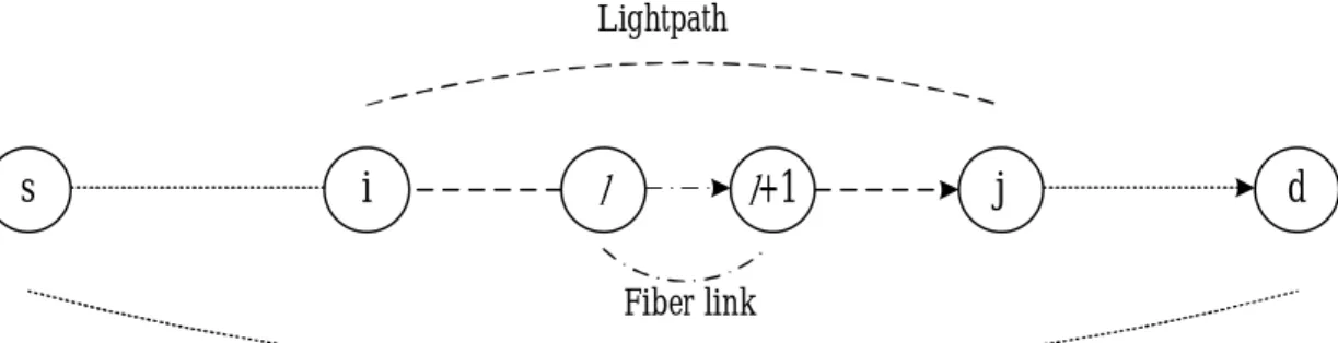
(19) rate λ (1/sec). Thus, the considered traffic model is traffic streams from any source and destination (s, d) arrive and leave according to Poisson process. A new traffic stream of type k is with probability pk, and its service time is exponentially distributed with mean service time 1/μk (sec). The destination of each traffic stream in the node uniformly locates among all the nodes in the considered network. As a result of our considered traffic model, the traffic streams will arrive one by one and the arrival time of next new call request is not known in advance. That is difference from the static traffic model. For the static traffic, the total traffic streams are given in advance.. 2.4 Problem Formulation for Traffic Grooming 2.4.1 Connection request, light path, fiber link, and the related notations Fig. 3 illustrates the relationship of connection request, lightpath and fiber link. A fiber link is a physical link between two adjacent nodes. A lightpath is an all optical channel which is used to carry circuit-switched traffic, and it may span multiple fiber links. Noted that a lightpath would occupy the same wavelength on all fiber links through which it passes, and multiple lightpaths with the same source and destination nodes are allowed. A connection request included source node and destination node can use multiple lightpaths. Before the mathematical problem formulation, three notation tables are given: Table 1 defines the notations, Table 2 defines the sets, and Table 3 defines the variables.. 10.

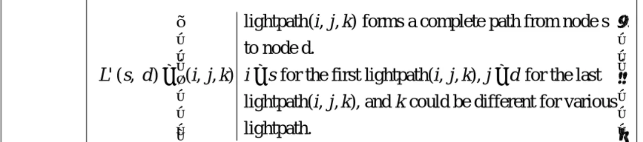
(20) Lightpath. s. i. +1. j. d. Fiber link Connection Request. Figure 3. Illustrative example of a fiber link, a lightpath and a connection request. Notation (i, j, k). Definition A lightpath which traverses from node i to node j through wavelength k without optical-electric conversion. i, j ∈ {1, 2..., N } , i ≠ j and 1≤ k ≤W .. (s, d). The node pair which represents source node s and destination node d for an end-to-end traffic. The end-to-end traffic may traverse through a single or multiple lightpaths. s , d ∈ {1, 2..., N } and s ≠ d .. N. The number of nodes in the network.. W. The number of wavelengths per fiber. We assume all the fibers in the network carry the same number of wavelengths.. C. Capacity of each wavelength (channel). C = OC-192.. m l. The maximum number of tunable transceiver pair equipped at each node. The fiber link between node l and node l+1. l ∈{1, 2,..., N } . l = N, if node. R. N to node 1. The required transmission capacity OC-R of a call. R ∈{1,3,12, 48} . Table 2.1: The notations of mathematical formulation. Set. Definition. L(i, j). Lightpath set which contains all the lightpaths from originating node i to terminating node j. L(i, j ) = {(i, j , k ) |1 ≤ k ≤ W }. B (l). Lightpath set which contains all the lightpaths pass through a given fiber. {. }. link l. B ( l ) = ( i, j , k ) lightpath ( i, j , k ) passes through fiber link l , ∀i, j L' (s, d). Lightpath set consists of successively non-overlapping linghpaths which form a complete path from node s to node d. Every element belongs to L' (s, d) can not pass through the same fiber link.. 11.

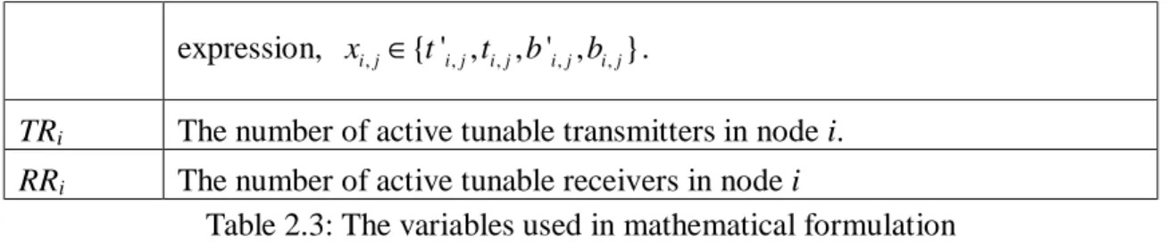
(21)     L ' ( s , d ) =  ( i, j , k )   . lightpath(i, j , k ) forms a complete path from node s   to node d.   i = s for the first lightpath(i, j , k ), j = d for the last  lightpath(i, j , k ), and k could be different for various   lightpath. . Table 2.2: The sets of mathematical formulation Variable t(i,j,k) (s, d). Definition The total traffic load in unit of OC-1 from (s, d) carried by the lightpath (i, j, k). t( i , j ,k ) ( s, d ) ∈ {0,1, 2,..., C} , for ∀( s, d ), (i, j, k ) .. ti,j. The total traffic load carried by the lightpaths belonging to L(i, j) before the acceptance of a new call request or the release of an on-going call. ti , j =. t'i,j. ∑. ∑. ( s , d ) ( i , j , k )∈L '( s , d ). t(i , j , k ) (s , d ) , for ∀( s, d ) .. The total traffic load carried by the lightpaths belonging to L(i, j) after the acceptance of a new call request or the release of an on-going call. i) If a new call with required traffic load R is accepted, t 'i , j = ti , j + R . ii). If an on-going call with required traffic load R releases, t 'i , j = ti , j - R .. c(i,j,k). The lightpath (i, j, k) indicator 1 a lightpath (i, j , k ) is actively used, i.e. (i, j, k ) ∈ L(i, j ) . c(i , j , k ) =  0 otherwise. bi,j. The number of wavelengths in L(i, j) before the acceptance of a new call request or the release of an on-going call, bi , j ∈ {0,1, 2,..., m} .. b'i,j. The number of wavelengths in L(i, j) after the accpetance of a new call request or the release of an on-going call, b 'i , j ∈ {0,1, 2,..., m} . The relationship between number of wavelengths and lightpath indicator W. can be described by the equation.. ∑c k =1. [ xi,j]. (i , j , k ). = b 'i , j , for ∀(i, j ) .. The N by N matrixes of which the (i, j)th element is xij, and x is the general. 12.

(22) expression, xi , j ∈{t 'i , j , ti , j , b 'i , j , bi , j } . TRi. The number of active tunable transmitters in node i.. RRi. The number of active tunable receivers in node i Table 2.3: The variables used in mathematical formulation. 2.4.2 Generalized Problem Formulation In this section, the dynamic traffic grooming in the metro ring network is formulated as an integer linear programming problem, where the design goal is to maximize the utilization efficiency of the wavelength used. This ILP problem is expressed as N. Maximize. t 'i , j. ∑ C *b '. i , j =1 i≠ j. ,. (2.1). i, j. subject to three constraints : (i). Traffic Constraint t 'i , j ≤ b 'i , j * C , for ∀(i, j ) ,. (2.2). ( ii ) Wavelength Constraints. ∑. b 'i , j ≤ W , for ∀l ,. (2.3). ∑. c(i , j ,k ) ≤ 1 , for ∀l , k ,. (2.4). ( i , j )∈B ( l ). ( i , j )∈B ( l ). ( iii ) Transceiver Constraints:. ∑b'. ≤ m , for ∀i ,. (2.5). ∑b'. ≤ m , for ∀j ,. (2.6). i, j. j. i, j. i. For traffic constraint, equation (2) indicates that the total traffic load from (i, j) must be less than the total capacity and relationship between the total traffic load and the lightpath count. For wavelength constraints, equation (3) expresses the bound imposed by the number 13.

(23) of wavelengths available while equation (4) ensures that no wavelength clash is allowed. For transceiver constraints, equation (5) and (6) ensure that the number of lightpaths from node i to node j is less than or equal to the number of transmitters and receivers, respectively. The above ILP problem is NP-complete [7]. Solving the ILP problem directly is not practical even for moderate-size networks because of the long computational time [13]. If the traffic model is static, the computational time may be negligible. Simple greedy heuristic and simulated-annealing algorithm [13], were proposed to obtain the optimization solution. However, considering dynamic traffic model, computational time is a critical issue. Some time-consuming optimization algorithms are not feasible to deal with dynamic traffic model. Alternatively, we propose a SA-based method for optimal solution and a heuristic-based method for suboptimal solution in the next chapter.. 14.

(24) Chapter 3 Optimal and Suboptimal Solutions to the Dynamic Traffic Grooming Problem. Chapter 3 Optimal and Suboptimal Solutions to the Dynamic Traffic Grooming Problem. T. his chapter presents an optimal and a suboptimal solution to the dynamic traffic problem stated in section 2.4.2. We first apply a SA algorithm to propose a. SA-based traffic grooming algorithm. The principle of SA and the STGA algorithm are described in section 3.1. We further propose a heuristic algorithm, called a heuristic-based traffic grooming (HTGA) algorithm, in section 3.2.. 3.1 Simulated Annealing-based Traffic Grooming Algorithm (STGA) In order to solve the dynamic traffic grooming problem (2.1), SA algorithm [16] is applied to obtain the optimal solution. In 1953, Metropolis proposed a method to simulate the annealing in physical sciences, and the concept of “Markov chain”, which each state was related to its previous state, was introduced. Until 1983, Kirkpatric applied the SA algorithm to solve NP-hard combinational optimization problem. For adapting the SA algorithm to the problem, a state of the Markov chain is defined as the matrix [bi', j ] which is the distribution of the lightapths in the network. The goal of the SA algorithm is to find an optimal matrix [bi', j ] having the maximum value of the object function, U, which is the sum of the utilization efficiency of the wavelength used.. 15.

(25)  N t 'i , j  MAX  U = ∑ i , j =1 C * b 'i , j  i≠ j .   ,  . (3.1). 3.1.1 The Concept and Procedure of SA The concept of SA is based on the manner in which liquids freeze or metals re-crystallize in the process of annealing. In an annealing process a melt, initially at high temperature and disordered, is slowly cooled so that the system at any time is approximately in thermodynamic equilibrium. As cooling proceeds, the system becomes more ordered and approaches a "frozen" ground state at temperature equaled zero. Hence the process can be regarded as an adiabatic approach to the lowest energy state. If the initial temperature of the system is too low or cooling is done insufficiently slowly the system may become quenched forming defects or freezing out in meta-stable states. From the concept of annealing, the general form of SA is described as follows.. Simulated Annealing ( [bi', j ]0 , Tmax ){ /* Given an initial state [bi', j ]0 and an initial value for the parameter T , Tmax */ T = Tmax ; [bi', j ] p = [bi', j ]0 ; While ( Outter loop criterion is not satisfied ) { While (Inner loop criterion is not satisfied ) { [bi', j ]q = Generate( [bi', j ] p ); If( Accept ( [bi', j ]q , [bi', j ] p , T ) ) { [bi', j ] p = [bi', j ]q ; } }. 16.

(26) T = Update(T ); } } The general form of SA algorithm involves five parameters: (I) The function Generate( [bi', j ] p ) is to select a new solution state [bi', j ]q according to the present state [bi', j ] p , (II) The function Accept ( [bi', j ]q , [bi', j ] p , T ) determines whether the new solution state [bi', j ]q is accepted according to a acceptance function fT (∆U pq ) . Its structure is shown below, Accept ( [bi', j ]q , [bi', j ] p ,T ){ /* The function returns a 1 if the cost variation passes a test. T is the control parameter */ ∆U pq = U q − U p ; y = fT (∆U pq ) ; r = random ( 0, 1); /* random is a function which returns a pseudo-random number uniformly distributed on the interval [0,1] */ If ( r < y ) return (1); Else Return (0); } The function Up represents the utility of the present state [bi', j ] p , while Uq represents the utility of the next state [bi', j ]q . The acceptance function fT (∆U pq ) is given by fT (∆U pq ) = min[1, exp(−. ∆U pq T. )] ,. which is a probability to accept the worse next state [bi', j ]q . 17. (3.2).

(27) (III) The function Update( T ) is to decrease the present temperature T to a new lower temperature with a decrement rate. (IV) Inner loop criterion is to decide whether sufficient number of moves has been tried to reach equilibrium condition at this temperature and T is about to decrease. (V) Outer loop criterion is used to test whether T is low enough to stop the SA algorithm.. 3.1.2 The Flowchart of STGA Fig. 4 shows the flowchart of STGA, which consists of three main processes: initialization, selection and comparison, and annealing.. Ÿ Initialization First of all, initial temperature, Tmax, final temperature, Tmin, decrement rate of temperature, γ, the maximum number of iteration at a temperature level, Lmax, should be set to appropriate values. Second, the initial matrix [bi', j ]0 is selected randomly and it must satisfy the constraints; if it does not satisfy, it is generated randomly again until it satisfied the constraints. Besides, the SA algorithm is insensitive to the initial state, so choosing a reasonable [bi', j ]0 in this case is enough for guaranteeing convergence of the STGA.. Ÿ Selection and Comparison The object function U is defined as the sum of the utilization efficiency of the wavelength used, and the goal is to find a reasonable matrix [bi', j ] to maximize U, which implies that maximizing the utilization efficiency of the wavelength used and satisfying the constraints at the same time. If [bi', j ] p = [bi', j ]0 , p denotes the present state, the next state [bi', j ]q will be generated from the neighborhood of [bi', j ]0 . If the next state [bi', j ]q is unreasonable, then it will be put in the taboo list to prevent to be chosen again in following iterations, and this makes STGA algorithm more efficient. If the next state [bi', j ]q is 18.

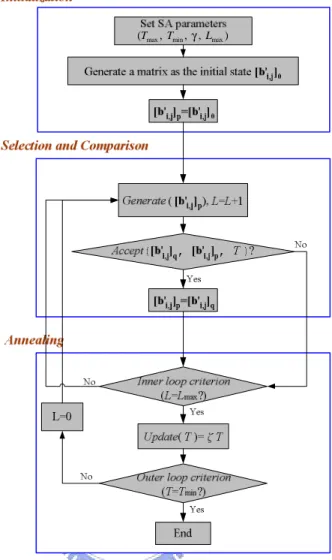
(28) reasonable, the SA algorithm will determine whether it accepts [bi', j ]q or not according to the acceptance function as follows, ∆U pq  ) exp( fT (∆U pq ) =  T 1 . if ∆U pq < 0. ,. (3.3). if ∆U pq ≥ 0. where ∆U pq = U q − U p . The [bi', j ]q will be absolutely accepted if Uq is larger than Up, or it will be accepted by probability. The significant advantage of the STGA algorithm comparing to greedy algorithm is that the SA algorithm gives a probability to accept a worse next state, because always choosing the better next state may lead to a suboptimal solution. The acceptance function fT (∆U pq ) in Fig.4 is the same as (3.3).. Ÿ Annealing If the number of iteration at a temperature level reaches Lmax, then the temperature will decrease by the decrement rate γ until the temperature reaches the final temperature Tmin. In initial stage of the SA algorithm, higher Tmax is appropriate to increase the probability of accepting a worse next state to prevent from falling into suboptimal solution. Moreover, high decrement rate γ reduces the tendency of accepting a worse next state quickly and makes fast convergence ; Low γ is on the contrary at the expense of convergence time.. 19.

(29) (Tmax , Tmin , γ , Lmax ). Figure 4. Flowchart of the Simulated Annealing-based Traffic Grooming algorithm. 3.2 Heuristic-based Traffic Grooming Algorithm (HTGA) Previous heuristic algorithms in papers [3], [4], [6-13], which focused on the static traffic model all, established lightpaths according to traffic given in advance. After the wavelengths ran out, traffic flows were grooming into the spare capacity which is the residual capacity of wavelengths. However, in the dynamic traffic model, the traffic can not be obtained in advance. It is insignificant that the approach establishes the lightpaths first. Besides, the problem formulation of the previous chapter describes the dynamic model as a static model according to the snapshot approach. However, the computational complexity remains unsolved. Thus, in order to maximize the utilization efficiency of the wavelength. 20.

(30) used and effectively reduce the new call blocking rate, a heuristic algorithm, called a heuristic-based traffic grooming algorithm (HTGA), is proposed. The heuristic ideas of HTGA states as follows: 1.. Traffic grooming or traffic assigned into a new lightpath (TG, TA) is performed for new call requests.. 2.. Traffic grooming and re-arrangement (TG, TA, TR) are performed when some lightpaths are under-utilized.. Basing on the idea mentioned above, we propose a heuristic algorithm for the heuristic-based traffic grooming algorithm (HTGA) to solve the generalized problem. The problem is divided into three subproblems: (a) traffic grooming subproblem, (b) wavelength assignments subproblem, (c) traffic rearrangement subproblem by the HTGA algorithm. As shown in Fig. 5, the block diagram of heuristic HTGA algorithm consists of traffic grooming (TG) block, wavelength assignment (WA) block, and traffic rearrangement (TR) block, which solve the (a), (b), (c) subproblems, respectively. The three subproblems are described in the following.. (a) Traffic grooming subproblem The utilization efficiency of the wavelength used increases as long as the traffic can be groomed into the lightpaths suitably. Thus, subproblem is considered as how to groom the traffic into lightpath suitably and find a suitable path for a call. Accordingly, we propose TG block that finds the lightpath of the lowest residual capacity first. The TG does not groom the traffic into random lightpaths. Instead, it finds the path from the wavelengths which the present lightpaths use, and considers the lowest residual capacity first. The path may be a present lightpath or a complete path which consists of more present lightpaths. TG block not only increases the utilization of wavelengths used but reduces the new call blocking rate.. 21.

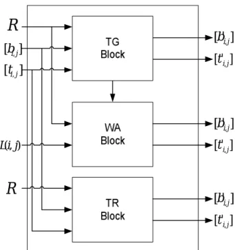
(31) (b) Wavelength assignment subproblem This subproblem is how to assign a wavelength to a lightpath suitably. Considering this subproblem, there exists a constraint: which any two lightpaths passing through the. same. physical. link. are. assigned. different. wavelengths.. Many. wavelength-assignment approaches were discussed in [14] and were found to perform similarly. Therefore, according to the results in [14], one simple approach, first-fit (FF), is selected to solve wavelength assignment subproblem. In FF, all wavelengths are numbered as 1, 2,…W, and if there is a lower numbered available wavelength, it will be considered first [15]. And, the FF is the WA block.. (c) Traffic rearrangement subproblem This subproblem is how to rearrange a portion of lightpaths topology suitably. In order to increase the performance of the network, we still consider the condition which it is possible that the present wavelengths are able to carry the traffic carried by the other wavelengths of lower utilization. Therefore, the TR of HTGA algorithm is to find the path for grooming the traffic which is carried by the other wavelengths of lower utilization into the path. The TR block can not only increase the utilization of wavelengths used but also reduce the new call blocking rate.. In next subsections, we introduce the operation of HTGA algorithm include three blocks and how the three blocks in HTGA algorithm search solution.. 3.2.1 Block Functionality In our work, our goals are to maximize the utilization efficiently of wavelengths which are occupied the current traffic stream in the network, and reduce the blocking rate of the. 22.

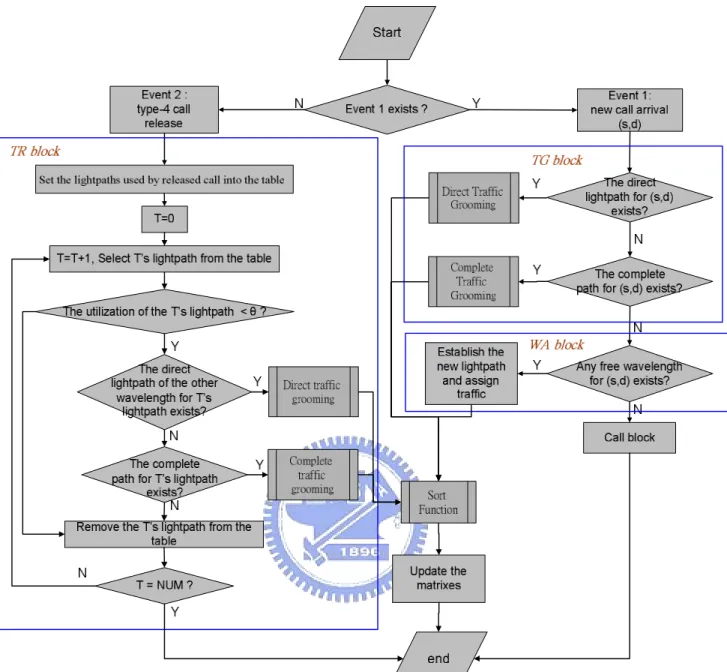
(32) new call request and computational time. Before discussing operation of HTGA, we describe the trigger events in HTGA. There are two events: event 1, event 2. Event 1 indicates new call arrival, and includes TG block and WA block of block diagram. In event 1, maximizing number of calls is achieved by TG and WA. Event 2 means type-4 call departure and includes TR block of block diagram. Because capacity of type-4 call is larger than the other types, the utilization efficiency of the wavelength may decrease largely when type-4 calls leaves. In event 2, maximizing efficiency of the wavelength used is achieved by TR. Now we will have a brief introduction of the operation of HTGA algorithm. The HTGA algorithm determines the matrixes, denoted by [b'i,j] and [t'i,j] which are defined in Table 2.3. The Fig. 5 shows the block diagram of HTGA algorithm. In the event 1, the new call request, the distribution of the present traffic and the present lightpaths are fed into TG block. The TG block calculates and outputs the matrixes [b'i,j] and [t'i,j]. If it can not calculate, the above data and information of wavelengths used are fed into WA block. The WA block calculates and outputs the matrixes [b'i,j] and [t'i,j]. In the event 2, the departure of traffic stream, the distribution of the present traffic, and the distribution of the present lightpaths are fed into TR block. If the rearrangement condition which the utilization is less than threshold value θ is achieved, the TR block calculates and outputs the matrixes [b'i,j] and [t'i,j]. If the rearrangement condition is not achieved, the TR block does not operate. θ means threshold value of utilization efficiency, θ ∈ {0.25, 0.5} .. 3.2.2 The Procedure The flowchart of the HTGA algorithm is shown in Fig. 6. From this flowchart, we describe how the three blocks in HTGA algorithm search solution. Before describing flowchart, some works will be defined and described.. 23.

(33) R. [b'i, j ]. [bi, j ]. [t 'i, j ]. [ti , j ]. [b'i, j ] [t 'i, j ]. L(i, j). R. [b'i, j ] [t 'i, j ]. Figure 5. The block diagram of HTGA algorithm. For initialization we assume that the matrixes [ti,j], [bi,j], [t'i,j], [b'i,j], and L(i, j) are all zero. The inputs are the new call request R, which is produced by source mode, [ti,j] and [bi,j] which equal to the output of the previous process, and L(i, j) which are recorded wavelengths used in previous process. The outputs are [t'i,j] and [b'i,j]. Now we introduce three functions in HTGA algorithm. When event 1 occurs, there are three steps. Step 1.1 and step 1.2 belong to the TG block, and the WA block consists of step 1.3.. – Step 1.1: Check (i, j,k) of the current lightpaths. If (i, j,k) of a lightpath which satisfies (s, d) of new call request exists and has enough capacity, the algorithm grooms traffic of new call to this lightpath, which is called direct lightpath and the utilization of lightpath is the largest than he other lightpaths with the same (s, d), and go to Step 1.4. Otherwise, go to Step 1.2. /*Find the direct lightpath to groom traffic: Start from the least available capacity of 24.

(34) wavelength*/ i := s; j := d; If (bi,j ≠ 0) { While( C - ti,j,k (s,d)> R) { Direct Traffic Grooming : { /*Groom R into the lightpath of the largest utilization*/ t'i,j = ti,j + R; Goto Sort Function (Step 1.4) } } } /*all current lightpaths do not be satisfied */ Else {Goto Step1.2}. – Step 1.2: Check complete paths. The algorithm tries to find the complete path which is composed of multiple current lightpaths and this path has enough capacity. If the complete path exists, the algorithm grooms traffic of new call to this path and go to Step 1.4. Otherwise, go to Step 1.3. /*Find complete paths to groom traffic: Start from the least available capacity of. 25.

(35) Wavelength*/ If (the distance between (s, d) ≤ N/2) { From i = s+1 to i = d-1 {. While (bi,j ≠ 0) {j := i; If (bid ≠ 0){ L’(s,d) ≠ 0; /*The complete path exists*/}} Break; }. } } Else /* the distance between (s,d) ≥ N/2 */ { i := s; From j = d+1 to j = s-1 { If (TRi ≠ m and RRi ≠ m) {While (bi,j ≠ 0) {L’(s,d) ≠ 0; /*The complete path exists*/} } } If (L’(s,d) ≠ 0) /*there is a complete path)*/ { Complete Traffic Grooming :. 26.

(36) {/*Groom R into the complete path.*/. ∑. i , j , k∈L '( s , d ). t 'i , j =. ∑. i , j , k ∈L '( s , d ). (ti , j + R). Goto Sort Function (Step 1.4) } } Else /*a complete path does not exist*/ {Goto WA block}. – Step 1.3: Check free wavelengths If the wavelengths which are not used from (s, d) exist, the algorithm will establish the new lightpath for new call and go to Step 1.4. Otherwise, new call is blocked and the algorithm ends. /*Check free wavelengths:*/ i :=s ,j := d If (L(i, j) ≠ W, TRi ≠ m and RRi ≠ m) { (i,j,k):=1;. k∉L(i, j);. /*Setup a new lightpath from node s to node*/ Goto Sort Function (Step 1.4)} Else /*there are not free wavelengths*/ { The call is blocked END }. – Step 1.4: Sort the utilization The algorithm will sort the utilization efficiency of the current lightpaths and update the matrixes. Then, the algorithm ends.. 27.

(37) Sort Function: According to the value of utilization of lightpaths, the current lightpaths are sorted in descendent order by the algorithm and the algorithm ends.. When event 2 occurs, there is one step which is included in TG block. – Step 2.1: Check the lightpath of released call If utilization efficiency of the lightpaths of departure call is small than θ, the algorithm will reroute lightpaths and groom traffic onto the other lightpath. The reroute condition is formed. Otherwise, the algorithm ends. /*Check the lightpath of released call and Groom the traffic load by the lightpaths of released call into the other lightpaths:*/ t'i,j = ti,j – R; Set the lightpaths used by released call into the table; NUM := the number of the lightpaths used by released call; T := 0 /*T is an iteration index of a for loop*/ From T = 0 to T = NUM. {Select T’s lightpath from the table If ((T’s lightpath load/192) < θ) {s := i; d := j; /*i and j belong to the lightpath (i, j, k)*/ R := traffic carried by the lightpath;. 28.

(38) /*Find the direct lightpath for T’s lightpath from the current Lightpaths*/ If ((i,j,k) ≠0 k∉T’s (i,j,k)) { Direct Traffic Grooming} Else { /*Find the complete path*/ If(L’(s,d) ≠ 0) {Complete Traffic Grooming} Else {Remove this lightpath from the table }}}} Else {Remove this lightpath from the table}} END;. 29.

(39) Figure 6. Flowchart of the HTGA algorithm. 30.

(40) Chapter 4 Performance Evaluation of the Proposed Algorithms. Chapter 4 Performance Evaluation of the Proposed Algorithms. I. n this chapter, simulation parameters are introduced in section 4.1 first. We evaluate the performance of HTGA algorithm and STGA algorithm in fixed network. configuration described in section 4.2.1. In order to reveal the performance of the algorithms with respects to various parameters, three kinds of scenario cases were simulated: Scenario 1: The number of nodes N is varied, but the other parameters are the same. Scenario 2: Mean service time 1/μk is varied, but the other parameters are always the same. Scenario 3: The ratio of the probability among difference type pk is varied, but the other parameters are always the same. The simulation results for the three cases are presented and discussed in section 4.2.2. Before discussing simulation results, we introduce how the parameters of STGA algorithm are obtained. The parameters of STGA algorithm are not always the same due to that they are determined by the other parameters of environment. Hence, the parameters of STGA algorithm are differently set according to the simulation environments. The relation between the parameters of STGA algorithm and the parameters of environment is expressed as [17]:. e e. ∆U max Tm in ∆U min Tmax. ≤ 0.01% ,. (4.1). ≥ 80% ,. (4.2) 31.

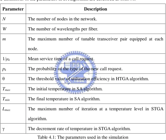
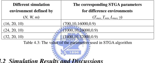
(41) Lmax = 100* N * N ,. (4.3). where ∆U max = −1/ C , if W < R, ∆U min = − N *W and if W ≥ R, ∆U min = − N * m . Tmax, Tmin and Lmax can be obtained from (4.1), (4.2) and (4.3). From [17], we select γ = 0.9.. 4.1 Simulation Parameters The definitions of the parameters in SA algorithm are described as follows: Description. Parameter N. The number of nodes in the network.. W. The number of wavelengths per fiber.. m. The maximum number of tunable transceiver pair equipped at each node.. 1/μk. Mean service time of a call request.. pk. The probability of the type of the new call request.. θ. The threshold value of utilization efficiency in HTGA algorithm.. Tmax. The initial temperature in SA algorithm.. Tmin. The final temperature in SA algorithm.. Lmax. The maximum number of iteration at a temperature level in STGA algorithm.. γ. The decrement rate of temperature in STGA algorithm. Table 4.1: The parameters used in the simulation. The value of the parameters, which are used in three cases by HTGA algorithm and STGA algorithm, are listed in Table 4.2, respectively. In table 4.3, the parameters of the STGA algorithm are computed according to above.. 32.

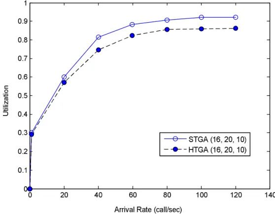
(42) Parameter. Values. N. 16, 24,32. W. 20. m. 10. 1/μk (sec). 60, 180. (p1, p2, p3, p4). (0.4, 0.3, 0.2, 0.1), (0.1, 0.2, 0.3, 0.4).. θ. 0.5 Table 4.2: The value of the parameters used in the simulation. Different simulation environment defined by (N, W, m). The corresponding STGA parameters for difference environments (Tmax, Tmin, Lmax, γ). (16, 20, 10). (700,10,16000,0.9). (24, 20, 10). (1000,10,24000,0.9). (32, 20, 10). (1400,10,32000,0.9) Table 4.3: The value of the parameters used in STGA algorithm. 4.2 Simulation Results and Discussions In this session, three performance measures for the HTGA algorithm and the STGA algorithm are discussed. The first is about the utilization efficiency of the wavelength of two algorithms. The second is about the new call blocking rate of two algorithms. The last is about the number of rearranged lightpaths of two algorithms when the new call is served. According to these issues, there are three kinds of graphs in simulation process.. 4.2.1 Performance Evaluation in Fixed Network Configuration Before discussing three cases between two algorithms, we first make the simulation comparison between the two algorithms executed the same environment. Fig. 7 and Fig. 9 show the utilization efficiency of the used wavelengths and the blocking ratio of the two. 33.

(43) algorithms, respectively. The utilization efficiency of the used wavelengths in the HTGA algorithm is only slightly less 10% than the STGA algorithm, and the blocking ration in the HTGA algorithm is only slightly higher 10% than the STGA algorithm. The STGA algorithm has better performance over the HTGA because it always finds the optimal allocation for every arrival call. Conversely, the HTGA algorithm just arranges every arrival call from the less residual capacity without changing the present lightpaths as could as possible, and it only rearranges traffic when the calls with large bandwidth request leaves the network.. Figure 7. The utilization efficiency of the used wavelengths in two algorithms. Fig. 9 illustrates two curves of the number of rearranged lightpaths for the two algorithms. As shown in the figure, the number of rearranged lightpaths in the STGA algorithm is larger than that in the HTGA algorithm. The reason is that, when a call is allowed to enter the network or departures from the network, the STGA algorithm rearranges all serving calls whereas the HTGA algorithm just rearranges parts of serving calls.. 34.

(44) Figure 8. The blocking ratio in two algorithms. Figure 9. Number of rearranged lightpaths per call in two algorithms. 35.

(45) However, the network has to take more time to establish the varied lightpaths if lightpaths are rearranged frequently. Lower number of rearranged lightpaths is preferable from the system’s point of view. In this aspect, the HTGA algorithm is more practical than the STGA algorithm obviously. Next, we discuss the computation complexity comparison between the STGA algorithm and the HTGA algorithm in the same environment. For the STGA algorithm, the arithmetic calculation can be de-composed into two parts: one is the number of the basic operations and the other is the number of the iteration. In addition, one iteration consists of many basic operations. Thus, the total number of the basic operations is the product of number of the basic operations and the number of iteration. The number of the basic operations is approximately ( χ *(N+N*W) ), where χ is the number of current served call. The complexity is represented as O( χ * N *W ) . Moreover, the total number of the iteration is Lmax * n from the principle of the SA algorithm, where n is the number of temperature level and given by ln Tmin − ln Tmax n= ln γ. (4.4). From (4.1) and ∆U min = 1/ C , we can calculate the number of temperature level for a constant Tmin . Besides, from (4.2) and ∆U max = − N *W , the Tmax is expressed as − N *W Tmax = ln(0.8). (4.5). According to (4.4), (4.5) and the constant Tmin, the complexity of n can be represented as O(ln( N *W )) . Also, the complexity of Lmax can be represented as O ( N 2 ) from (4.3). Therefore, the complexity of the total number of the iteration is derived by O (ln( N *W ) * N 2 ) , and he overall computation complexity of STGA is represented as O (ln( N *W ) * χ * N 3 *W ) according to results of two parts. In the HTGA algorithm, the number of the basic operations for event 1 is approximately (2N+2*N*W) and the one for event 2 is approximately (N*(2*N+2*N*W)). Thus, the. 36.

(46) complexity of the HTGA algorithm is represented as O( N 2 *W ) . For example, if the CPU of the computer is 3GHz, each clock time costs 1/3 nanosecond. From two algorithms, the number of clock time in the iteration is estimated to be 20. Then, the STGA algorithm costs approximate 0.72 second to obtain solution and the HTGA algorithm costs approximate 5.5 microsecond. Obviously, the difference in computation complexity between two algorithms is pretty large. With the results, we can conclude that the STGA algorithm requires very large computation power although it can attain optimal solution. However, the HTGA algorithm can attain acceptable system utilization close to the STGA algorithm while its computation complexity is extremely low. Moreover, the HTGA algorithm only has to change a small portion of lightpaths, compared to the SA algorithm.. Thus, the HTGA algorithm effectively. reduces the computation complexity without severely suffering the system utilization, making it more practical and implementation-feasible for the current optical equipments.. 4.2.2 Performance Evaluation in Various Network Configurations After discussing the two algorithms executed in the fixed environment, the three scenario cases are then discussed to evaluate the algorithms under various parameter settings. Fig. 10 and Fig. 11 show the results of the utilization efficiency of the used wavelengths and the blocking ratio for Scenario 1, respectively. When number of nodes increases, the HTGA algorithm can still attain high system utilization, compared to the STGA algorithm. In addition, the utilization curves of two algorithms reach the saturation state at lower arrival rate as number of nodes increases. The reason is that the optical network accommodates more service calls at the saturation state when the network size enlarges.. 37.

(47) Figure 10. The utilization efficiency of the used wavelengths in Scenario 1. Figure 11. The blocking ratio in the Scenario 1. 38.

(48) The results of the Scenario 2, including the utilization efficiency of the used wavelengths and the blocking ratio, are shown in Fig. 12 and Fig. 13, respectively. As mean service time increased, the curve of utilization efficiency reaches the saturation state at a lower arrival rate. Moreover, as mean service time becomes larger, the utilization gap between the two algorithms widens, and so as the blocking ratio. The reason is that the number of serving call in the network becomes large with the same arrival rate and also the chances of rearranged traffic decrease due to the lower trigger probability of event 2.. Figure 12. The utilization efficiency of the used wavelengths in Scenario 2. In Scenario 3, two type of new call request (p1, p2, p3, p4) are simulated. One is (0.4, 0.3, 0.2, 0.1), called small-call case. The other is (0.1, 0.2, 0.3, 0.4), called large-call case. Type-1 users have the highest new call arrival probability in the small-call case while Type-4 users have the highest new call arrival probability in the large-call case.. 39.

(49) Figure 13. The blocking ratio in the Scenario 2. Fig. 14 shows the utilization efficiency of the used wavelengths of two algorithms. The arrival rate to reach saturation in the small-call case is higher than that in the large-call case; moreover, the utilization gap between the two algorithms in the large-call case is smaller than that in the small-call case. The large-call case accommodates more type-4 calls so that it has a larger total traffic load and higher chances to trig the rearrangement event. As a result, the system performance in the large-call case is better. Fig. 15 shows the blocking ratio of two algorithms. The blocking ratio of large-call case is higher than that of the small call case. The reason is the same as the above-mentioned one. As shown in Fig. 10 to Fig. 15, the simulation results reveal that the throughput gap between the two algorithms is no more than 10% in all the three Scenarios. Thus, we can conclude that the performance of the HTGA algorithm does not deteriorate substantially in various environments, including different network size, mean service time, and probability of new call request type. Therefore, the HTGA algorithm is an attractive and feasible algorithm.. 40.

(50) Figure 14. The utilization efficiency of the used wavelengths in Scenario 3. Figure 15. The blocking ratio in the Scenario 3. 41.

(51) Chapter 5 Conclusion. Chapter 5 Conclusion. In this thesis, we are motivated to solve the problem of dynamic traffic grooming and wavelength assignment in metro-access ring network. The goal is to effectively maximize the utilization efficiency of the wavelength used and reduce the new call blocking rate. We first study the architecture of node with grooming capacity and network architecture. Then, we also present the ILP formulation for the problem. In order to solve this problem, we propose STGA algorithm to obtain the optimal solution. However, the STGA algorithm is infeasible due to its computation complexity. Alternatively, we propose a heuristic algorithm-based HTGA algorithm. Although the HTGA algorithm is a suboptimal solution, the computation complexity of the HTGA is much lower than that of the STGA. From the simulation comparisons between the two algorithms in the same environment, we can summarize the pros and cons of the STGA and HTGA algorithm. For STGA algorithm, the advantage is that it can attain an optimal solution while the disadvantage is that the computation complexity and the number of rearranged lightpaths are large. On the other hand, for HTGA algorithm, the advantage is that the computation complexity and the number of rearranged lightpaths are small while the disadvantage is that it just can obtain sub-optimal solution. However, the disadvantage of the HTGA algorithm is accepted because the gap of the throughput utilization is just less than 10%. Therefore, the HTGA algorithm is a feasible and attractive algorithm. Besides, another advantage of the HTGA can be observed in various environments. Simulation results show that the throughput gap between the two algorithms is no more than 42.

(52) 10% in all the three Scenarios. Thus, we can conclude that the performance of the HTGA algorithm does not deteriorate substantially in various network configurations, including different network size, mean service time, and probability of new call request type. Therefore, the results demonstrate once again the superiority of the HTGA algorithm.. 43.

(53) Bibliography [1] B. Mukherjee, S. Ramamurthy, D. Banerjee, and A. Mukherjee, “Some principles for designing a wide-area optical network,” Proc. of IEEE INFOCOM ‘94, vol. 1, pp. 110 – 119, June 1994. [2] E. Modiano and P. J. Lin, “Traffic grooming in WDM networks,” IEEE Comm. Mag., vol. 39, no. 7, pp. 124 – 129, July 2001. [3] K. Zhu, and B. Mukherjee, “Traffic grooming in an optical WDM mesh network,” IEEE Journal on Selected Areas in Communications, vol. 20, no. 1, pp.. 122 – 133, Jan.. 2002. [4] R. Dutta, and G.. Rouskas, “On optimal traffic grooming in WDM rings,” IEEE Journal on Selected Areas in Communications, vol. 20, no. 1, pp. 110 – 121, Jan. 2002. [5] D. Li, Z. Sun, X. Jia, and K. Makki “Traffic grooming on general topology WDM networks,” IEE Proc. Commun., vol. 150, no.3, pp. 197 – 201, June. 2003. [6] B. Chen, G. Rouskas, and R. Dutta “Traffic grooming in WDM ring networks with the min-max objective,” Proceedings of Networking 2004, pp. 174 – 185, May. 2004. [7] E. H. Modinao, and A. L. Chiu “Traffic grooming algorithms for reducing electronic multiplexing costs in unidirectional WDM ring network,” Journal of Lightwave Technology , vol.18, no. 1, pp. 2-12, Jan. 2000. [8] X. Zhang, and C. Qiao “An effective and comprehensive solution to traffic grooming and wavelength assignment in SONET/WDM rings,” IEEE/ACM Transactions Journal on Networking, vol. 8, no. 5, pp. 608-617, Oct. 2000. [9] Moon-Gil Yoon “Traffic grooming and light-path routing in WDM ring networks with hop-count constraint,” IEEE International Conference on Communications, vol. 3, pp. 731-737, June 2001.. 44.

(54) [10] V.R. Konda, and T.Y. Chow “Algorithm for traffic grooming in optical networks to minimize the number of transceivers,” IEEE Workshop on High Performance Switching and Routing, pp. 218-221, May 2001. [11] P. Prathombutr, J. Stach, and E.K. Park “An algorithm for traffic grooming in WDM optical mesh networks with multiple objectives,” ICCCN 2003, pp. 405-411, Oct. 2003. [12] R.B. Billah, B. Wang, and A.S. Awwal “Efficient traffic grooming in synchronous optical network/wavelength-division multiplexing bidirectional line-switched ring network,” Optical Engineering, vol. 43, no. 5, pp. 1101-1114, May 2004. [13] J. Wang, W. Cho, V. R. Vemuri, and B. Mukerjee “Improved approaches for cost-effective traffic grooming in WDM ring networks: ILP formulations and single-hop and multiple connections,” Journal of Lightwave Technology, vol. 19, no.11, pp. 1645 – 1653, November. 2001. [14] H. Zang, J. P. Jue, and B. Mukerjee “A review of routing and wavelength assignment approaches for wavelength-routed optical WDM network,” Optical Network Mag., vol. 1, no.1, pp. 47 – 66, Jan. 2000. [15] X. Sun, Y. Li, I. Lambadaris, and Y.Q. Zhao “Performance analysis of first-fit wavelength assignment algorithm in optical networks,” Telecommunications, 2003. ConTEL 2003, vol. 2, no.1, pp. 403 – 409, June. 2003. [16] F. I. Romeo, “Simulated Annealing: Theory and applications to layout problems”. Memorandum No. UCB/ERL M89/29, March 1989. [17] S. Kirkpatrick, C. D. Gellatt, and M. P. Vecchi. “Simulated annealing.” Science, 220, 1983.. 45.

(55) Vita 姓名：郭朕逢學歷： 2003 ~ 2005 交通大學電信工程研究所 1998 ~ 2002 長庚大學電子工程學系 1995 ~ 1998 私立黎明高級中學. E-mail: [email protected]. 46.

(56)