A Parallel Loop Scheduling for Extremely Heterogeneous PC Clusters

全文

(1)A Parallel Loop Scheduling for Extremely Heterogeneous PC Clusters Chao-Tung Yang and Shun-Chyi Chang High-Performance Computing Laboratory Department of Computer Science and Information Engineering Tunghai University Taichung, 407, Taiwan, R.O.C. Tel: +886-4-23590121#3279 [email protected]. Abstract. Cluster computers are becoming increasingly more common, especially with the increasing use of Beowulf systems, and networks of workstations (NOW) for parallel computing. Nowadays using cost-effective cluster computers to deal with problems which need large computing is a spreading trend. The major source of parallelism in a program is loops. If the loop iterations can be distributed to different processors evenly, the parallelism within loop iterations can be exploited. In homogeneous environment, one can divide equal amount of iterations to each processor, but in heterogeneous environment, this way is not suitable. Self-scheduling schemes, such as FSS, GSS and TSS, can achieve load balancing in SMP, even in moderate heterogeneous environment, but are not suitable in extremely heterogeneous environment. In this paper, we propose a heuristic approach to solve parallel loop scheduling problem in extremely heterogeneous environment. The experiments were conducted on a heterogeneous PC cluster.. 1. Introduction Parallel computers are becoming increasingly widespread, and nowadays many of these parallel computers are no longer shared-memory multiprocessors, but rather follow the distributed memory model for scalable. These systems may consist of homogeneous workstations, where all the workstations have processors with exactly the same specifications and identical memory and caches. However, increasingly systems are now composed of a number of heterogeneous workstations clustered together, where each workstation may have CPUs with different performance capabilities and different amounts of memory and caches, and even different architectures and operating systems. To exploit the potential computing power of cluster computers, an important issue is how to assign tasks to computers so that the computer loads are well balanced. The problem is how to assign the different parts of a parallel application to the computing resources to minimize the overall computing time and to efficiently use the resource. An efficient approach to extract potential parallelism is to concentrate on the parallelism available in the loops. Since the body of a loop may be executed many times, loops often comprise a large portion of a program’s parallelism. By definition, a loop is called a DOALL loop if there is no cross-iteration dependence in the loop; i.e., all the iterations of the loop can be executed in parallel. If all the.

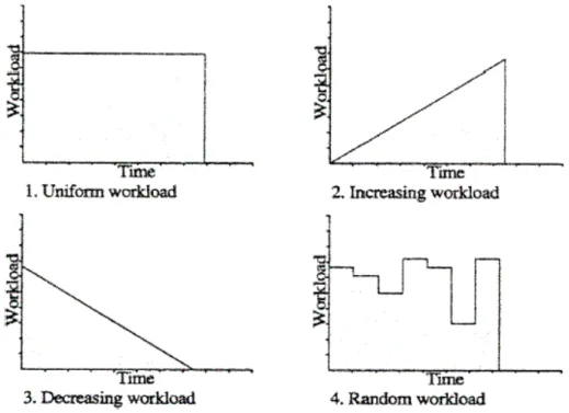
(2) iterations of a DOALL loop are distributed among different processors evenly, a high degree of parallelism can be exploited. Parallel loop scheduling is a method that attempts to evenly schedule a DOALL loop on multiprocessor systems. According to Moore’s law, CPU clock will double in 18 months and this law still works today. We may have to build clusters consisting of extremely different computer performance. In homogeneous environment, workload can be partitioned equally to each working computer, but in heterogeneous environment, this method will not work. Some researches were proposed to solve parallel loop scheduling problems on heterogeneous cluster environments by using selfscheduling schemes. These self-scheduling schemes will work well in moderate heterogeneous cluster environment but not in extremely heterogeneous environment where the performance difference between the fastest computer and the slowest computer is larger than double of working computers. In this paper, we will propose a loop scheduling based on self-scheduling scheme to approach load balancing on extremely heterogeneous cluster. The experimental results are conducted on a PC Cluster with six nodes and the fastest computer is 7.5 times faster than the slowest ones in CPU-clock. In our experiments, we assign 80% workload corresponding to the CPU clock, and 20% workload using traditional self-scheduling to achieve a good load balancing. The rest of the paper is organized as follows. In section 2, a brief overview of self-scheduling is given. Section 3 states our approach and reports the experiments. Finally, the conclusion remarks are given in section 4.. 2. Background Loops are one of the largest sources of parallelism in scientific programs, and thus a lot of research work focused on this area. Parallel loop scheduling is used to achieve this goal by determining how to assign the DOALL loops onto each processor in a balanced fashion so as to achieve a high level of parallelism with the least amount of overhead. In a parallel process system, two kinds of parallel loop scheduling decisions can be made either statically at compiletime or dynamically at run-time. Static scheduling is usually applied to uniformly distributed iterations on processors [6]. However, it has the drawback of creating load imbalances when the loop style is not uniformly distributed; when the loop bounds cannot be known at compile-time; or when locality management cannot be exercised. In contrast, dynamic scheduling is more appropriate for load balancing; however, the runtime overhead must be taken into consideration. In general, parallelizing compilers distribute loop iterations by using only one kind of scheduling algorithm, which maybe static or dynamic. However, a program may have different loop styles, such as uniform workload, increasing workload, decreasing workload, or random workload..

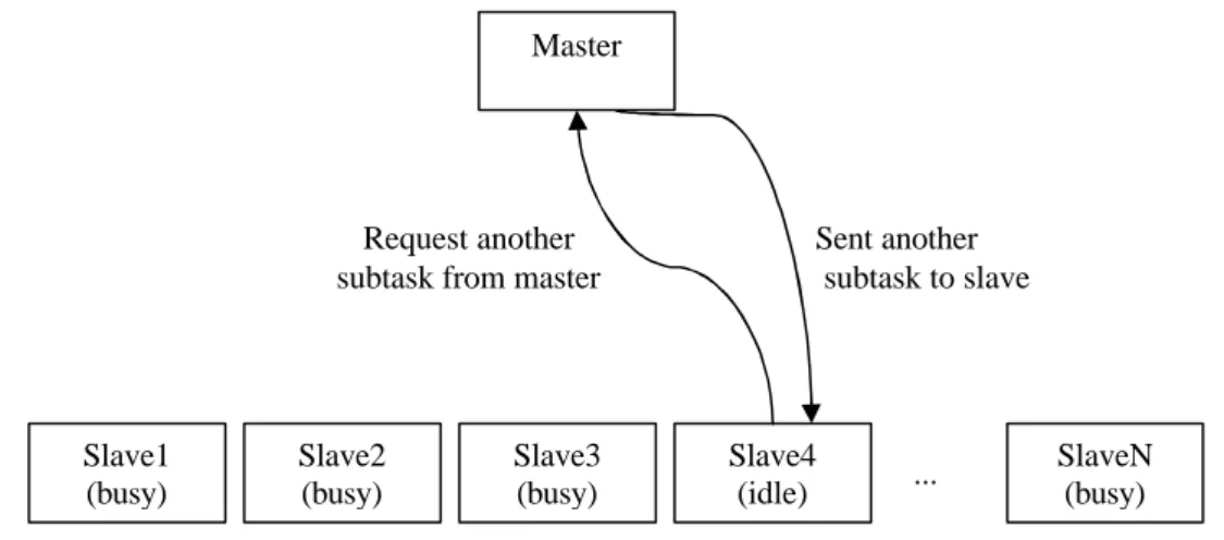
(3) 2.1 Static Scheduling Traditional static scheduling [6] makes a scheduling decision at compile-time and uniformly distributes loop iterations onto processors. It is applied when each loop iteration takes roughly the same amount of time, and the compiler knows how many iterations will be run and how many processors are available for use at compile-time. It has the advantage of incurring the minimum scheduling overhead, but load imbalances may occur. These static scheduling schemes including Block Scheduling, Cyclic Scheduling, Block-D Scheduling, Cyclic-D Scheduling…. etc [6]. But these scheduling schemes were unsuitable in heterogeneous. environment. Theoretically, workload can be partitioned according to their computer performance. Unfortunately, in heterogeneous system, it is important to evaluate each computer performance, but it is not easy. Intuitively, CPU clock speed may be a good evaluation value. But it seems not enough. Many factors affect computer performance, such as the performance capability of the CPU, the amount of memory available, the cost of memory accesses, the communication medium between processors… etc [5]. Bohn and Lamont try to evaluate the performance of computer in compiler-time [4]. In their experiment, HINT is a good benchmark. It evaluates processor and memory performance for any data type and returns a single value, ‘QUIPS’. Bohn and Lamont declared ‘QUIPS’ can present the computer performance. It has the advantage of all computers being working computer - no control computer is needed. But, HINT requires hours to execute, it means this way will not be scaling well. It takes a long time to add one more computer and if we want to change the peripheral, for example to replace RAM from pc100 to pc133, we might have to rerun HINT.. 2.2 Dynamic Scheduling Dynamic scheduling adjusts the schedule during execution whenever it is uncertain how many iterations to expect or when each iteration will take a different amount of time due to a branching statement inside the loop. Although it is more suitable for load balancing between processors, runtime overhead and memory contention must be considered. Self-scheduling is a large class of adaptive/dynamic centralized loop scheduling schemes. We will study these schemes from the perspective of distributed systems. For this, we use the master-slave architecture model: idle slave PCs communicates a request to the master for new loop iterations. The number of iterations a PC should be assigned is an important issue. Due to PCs heterogeneity and communication overhead, assigning the wrong PC a large number of iterations at the wrong time may cause load imbalancing. Also, assigning a small number of iterations may cause too much communication and scheduling overhead. Although dynamic.

(4) scheduling may achieve load balancing, a master computer which be responsible for assigning subtask to slave is needed. Master computer is not responsible for workload.. Master. Request another subtask from master. Slave1 (busy). Slave2 (busy). Slave3 (busy). Sent another subtask to slave. Slave4 (idle). .... SlaveN (busy). Figure 1: A master/slave model. In a generic self-scheduling scheme, at the ith scheduling step, the master computers the chunk-size Ci and the remaining number of tasks Ri, R0=I, Ci=f(Ri-1,p), Ri=Ri-1-Ci where f(,) is a function possibly of more inputs than just Ri-1 and p. Then the master assigns to a slave PC Ci tasks. Imbalancing depends on the (execution time gap) between tj, for j=1,… ,p. This gap may be large if the first chunk is too large or (more often) it the last chunk (called the critical chunk) is too small [7]. The different ways to compute Ci has given rise to different scheduling schemes. The most notable examples are the following. Pure Self-Scheduling (SS) This is the easiest and most straightforward dynamic loop scheduling algorithm [9]. Whenever a processor is idle, an iteration is allocated to it. This algorithm achieves good load balancing but also introduces excessive overhead. Chunk Self-Scheduling (CSS) Instead of allocating one iteration to an idle processor as in self-scheduling, CSS allocates k iterations each time, where k, called the chunk size, is fixed and must be specified by either the programmer or the compiler [8]. When the chunk size is one, this scheme is pure self-scheduling, as discussed above. If the chunk size is set to the bound of the parallel loop equally divided by the number of processors, the scheme becomes static scheduling. A large chunk size will cause load imbalancing while a small chunk is likely to produce too much scheduling overhead. For different partitioning schemes, we adapted CSS/l, which is a modified version of CSS, where l means the number of chunks. Guided Self-Scheduling (GSS) This algorithm can dynamically change the number of iterations assigned to each processor [2]. More specifically, the next chunk size is determined by.

(5) dividing the number of remaining iterations of a parallel loop by the number of available processors. The property of decreasing chunk size implies an effort is made to achieve load balancing and to reduce the scheduling overhead. By allocating large chunks at the beginning of a parallel loop, one can reduce the frequency of mutually exclusive accesses to shared loop indices. The small chunks at the end of a loop partition serve to balance the workload across all the processors. Factoring In some cases GSS might assign too much work to the first few processors, so that the remaining iterations are not time-consuming enough to balance the workload. This situation arises when the initial iterations in a loop are much more time-consuming than later iterations. The factoring algorithm addresses this problem [1]. The allocation of loop iterations to processors proceeds in phases. During each phase, only a subset of the remaining loop iterations (usually half) is divided equally among the available processors. Because Factoring allocates a subset of the remaining iterations in each phase, it balances loads better than GSS does when the computation times of loop iterations vary substantially. In addition, the synchronization overhead of Factoring is not significantly larger than that of GSS. Trapezoid Self-Scheduling (TSS) This approach tries to reduce the need for synchronization while still maintaining a reasonable load balance [3]. TSS(Ns, Nf) assigns the first Ns iterations of a loop to the processor starting the loop and the last Nf iterations to the processor performing the last fetch, where Ns and Nf are both specified by either the programmer or the parallelizing compiler. This algorithm allocates large chunks of iterations to the first few processors and successively smaller chunks to the last few processors. Tzen and Ni proposed TSS(N/2P, 1) as a general selection. In this case, the first chunk is of size. size. N , and consecutive chunks differ in 2p. N iterations. The difference in the size of successive chunks is always a constant in TSS 8 p2. whereas it is a decreasing function in GSS and in Factoring. Table 1 shows the different chunk sizes for a problem with I=1000 and p=4. Scheme PSS CSS(125) FSS GSS TSS. Partition size 1,1,1,1,1,1,1… 125,125,125,125,125,125,125,125 125,125,125,125,63,63,63,63,31,31,31,31, 250,188,141,106,79,59,45,33,25,19… 125,117,109,101,93,85,77,69,61,53… Table 1: Sample partition sizes.

(6) 3. Our Approach In extremely heterogeneous environment, cluster computers have extremely different performance. In this condition, additional slave computers may not get good performance because these known self-scheduling schemes partition size of loop iteration according to formula instead of computer performance. In FSS, for example, every slave gets a size of N/2p workload, where N is the total of workload; p is the number of processor. If the performance difference between the fastest computer and the slowest computer is larger than N/2p, then load imbalance happens. Furthermore, dynamic load balancing should not be aware of the run-time behavior of the applications before execution. But in GSS and TSS, to achieve good performance, computer performance has to be ordered in extremely heterogeneous environment. A combination of machine types is used to test the behavior of these techniques in a heterogeneous computing environment, and the matrix multiplication is chosen as the test application to get a heuristic result due to its regular behavior. This experiment included 4 computers. One of them is assigned as master using TSS. The master is a PC with 300 MHz CPU and 208MB physical memory. The three slaves are PCs, respectively, with 1.5GHz CPU and 256MB physical memory, 233 MHz CPU and 96MB physical memory, and 200MHz CPU and 64MB physical memory. The slaves are added sequentially in this order. We use TSS and FSS to test matrix multiplication with 512*512, 1024*1024, and 2048*2048 floating point operation. Table 2 shows our experiment result. Note that just one slave in table 2 means that all work is done by the fastest computer only. We can see the performance of two slave computers is less than the performance of one high speed slave computer.. No. of slaves. Execution time(TSS) 512*512. Execution time(FSS). 1024*1024 2048*2048 512*512. 1024*1024 2048*2048. 1 0'12''066. 1'44''357. 17'12''483 0'12''136. 1'44''688. 17'11''402. 2 0'17''520. 2'49''652. 19'34''016 0'18''371. 3'16''561. 23'48''723. 3 0'13''339. 1'53''202. 16'30''651 0'14''543. 2'00''491. 16'36''007. Table 2: The result performance of number of slaves in extremely heterogeneous environment. As mentioned above, in heterogeneous environment, intuitively, we may want to partition problem size according to their CPU clock. However, the CPU clock is not the only factor which affects computer performance. Many other factors also have dramatic influences in this aspect, such as the amount of memory available, the cost of memory accesses, the communication medium between processors… etc. Using this intuitive approach, the result will.

(7) be degraded if the performance prediction is accurate. A computer with largest inaccurate prediction, being the last one to finish the assigned job, is called the dominate computer. We propose to partition the a% of workload according to their performance weighted by CPU clock and the (100-a)% of workload according to known self-scheduling scheme. To get load balancing, we make the (100-a )% of workload wait the dominate computer until it finishes its job. Using this approach, we don’t have to know the real computer performance. The computer finishing its job early gets a larger job to wait for the slower computer. Another advantage of using this approach is the reduction of communication. When this approach is applied to the matrix multiplication, with a=80, a better performance is obtained. Loops can be roughly divided into four kinds as shown in figure 2: uniform workload, increasing workload, decreasing workload, and random workload loops. They are the most common ones in programs, and should cover most case. These four kinds can be classified two types: predictable and unpredictable. Our approach is suitable in all applications with predictable loops.. Figure 2: Four kinds of loops. Algorithms MASTER and SLAVE in pseudo code: Module MASTER /* performs task scheduling and load balancing */ Initialization Gather CPU clock of all slave computers r=0; For (i=1; i<number_slave; i++) { Partition α% of loop iteration corresponding their CPU clock speed and sent data to slave r++;.

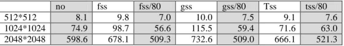
(8) } Partition (100-α)% of loop iteration into task queue using some known self-scheduling scheme Probe if some data in Do{ Distinguish source and receive data If task queue not empty Sent other data to this idle slave r--; Else sent TAG=0 to this idle slave }while (r>0); Finalization END MASTER Module SLAVE /* worker */ Initialization Sent my CPU clock to master Probe if some data in While (TAG>0){ Receive initial solution and size of subtask work and compute to find solution Send the result to master Probe if some data in } Finalization END SLAVE. The approach is applied in an extremely heterogeneous environment which includes 6 computers. One of them is assigned as the master. The master is a PC with 300 MHz CPU and 208MB physical memory. Two of the slaves are PCs with 200 MHz CPU and 64 MB physical memory. The other three slaves are PCs, respectively, with 233 MHz CPU and 96MB physical memory, 533MHz CPU and 128MB physical memory, and 1.5GHz CPU and 256MB physical memory. Those computers may own various NIC and cost of memory access, regarding as part of computer performance. SWAP occurs in some computers. If not serious, this will not affect the result. The parameter a should not be too small or too big. In former case, the dominate computer will not finish its work and then leads to bad performance. In the latter case, the dynamic scheduling strategy is rigid. In both cases, good performance can not be attained. An appropriate a value will lead to good performance and reduce communication times. Many a values are applied to the experiments, and a=80 result in the best performance. Table 3 and Figure 3 show the result in a=80. The column name ‘no’ stands for ‘no loadbalancing’ and workload be partitioned just by CPU clock. ‘fss/80’ stand for ‘a=80, and remainder use fss to partition’ and so on. In our case, using this approach in 2048*2048 matrix multiplication will get 25%, 30%, 21% performance improvement than FSS, GSS, TSS respectively. Note that in extremely heterogeneous environment, known self-scheduling get worse performance than schemes partitioning workload merely according to the CPU clock..

(9) no 512*512 1024*1024 2048*2048. fss 8.1 74.9 598.6. 9.8 98.7 678.1. fss/80 7.0 56.6 509.3. gss 10.0 115.5 732.6. gss/80 7.5 59.4 509.0. Tss 9.1 71.6 666.1. tss/80 7.6 63.0 521.3. Processing time (sec). Table 3: The result of our approach in extremely heterogeneous environment (a=80). 800 700 600 500 400 300 200 100 0. no fss fss/80 gss gss/80 tss tss/80 512*512. 1024*1024. 2048*2048. Problem size Figure 3: The result of our approach in extremely heterogeneous environment (a=80). Our approach is also useful in moderate environment. Following experiment includes 5 computers. One of them is assigned as the master. The master is a PC with 900 MHz CPU and 256MB physical memory. Two of the slaves are PCs with 200 MHz CPU and 64 MB physical memory. The other two slaves are PCs, respectively, with 975 MHz CPU and 512MB physical memory, 900MHz CPU and 256MB physical memory. Two of slaves are PCs with 600GHz CPU speed and 256MB of physical memory. Table 4 and Figure 4 present the result when the approach is applied to matrix multiplication, as a = 80. It shows that our approach has equal or better performance than the known self-scheduling.. 1024*1024 2048*2048 3072*3072. no 64.6 520.8 1792.8. fss 59.1 477.3 1720.9. fss/80 59.1 474.4 1711.0. gss 59.1 477.6 1715.8. gss/80 59.0 474.3 1714.7. tss 65.2 505.8 1792.1. Table 4: The result of our approach in moderate heterogeneous environment (a=80).

(10) Processing time (sec). 2000 1800 1600 1400 1200 1000 800 600 400 200 0. no fss fss/80 gss gss/80 tss. 1024*1024. 2048*2048. 3072*3072. Problem size Figure 4: The result of our approach in moderate heterogeneous environment (a=80). 4. Conclusion and future work In extremely heterogeneous environment, known self-scheduling schemes can not achieve good load balancing. In this paper, we propose an approach to partition loop iterations and achieve good performance in such environment: partitioning the 80% of workload according to their performance weighted by CPU clock and the 20% of workload according to known selfscheduling. Using our approach in 2048*2048 matrix multiplication will get 30% performance improvement than GSS. Our approach is suitable in all applications with predictable loops. In near future, we will try to solve parallel loop scheduling problems with unpredictable loops.. References [1] S. F. Hummel, E. Schonberg, L. E. Flynn, “Factoring, a Scheme for Scheduling Parallel Loops”, Communications of the ACM, Vol 35, No 8, Aug. 1992. [2] C. D. Polychronopoulos and D. Kuck, “Guided Self-Scheduling: a Practical Scheduling Scheme for Parallel Supercomputers”, IEEE Trans. on Computers, Vol 36, Dec. 1987, pp 1425 - 1439. [3] T. H. Tzen and L.M. Ni, “Trapezoid Self-Scheduling: A Practical Scheduling Scheme for Parallel Compilers”, IEEE Trans. on Parallel and Distributed Systems, Vol 4, No 1, Jan. 1993, pp 87 - 98. [4] Christopher A. Bohn, Gary B. Lamont, “Load Balancing for Heterogeneous Clusters of PCs”, Future Generation Computer Systems 18 (2002) 389–400.

(11) [5] E. Post, H. A. Goosen, “Evaluating the Parallel Performance of a Heterogeneous System”, in the Proceedings of HPCAsia2001 [6] H. Li, S. Tandri, M. Stumm and K. C. Sevcik, “Locality and Loop Scheduling on NUMA Multiprocessors,” in Proceedings of the 1993 International Conference on Parallel Processing, Vol. II, 1993, pp. 140-147. [7] A. T. Chronopoulos, R. Andonie, M. Benche and D.Grosu, “A Class of Loop SelfScheduling for Heterogeneous Clusters,” in Proceedings of the 2001 IEEE International Conference on Cluster Computing [8] T. H. Tzen and L. M. Ni, “Trapezoid self-scheduling: A practical scheduling scheme for parallel compilers,” IEEE Transactions on Parallel Distributed Systems, Vol. 4, No. 1, 1993, pp. 87-98. [9] P. Tang and P. C. Yew, “Processor self-scheduling for multiple-nested parallel loops, ” in Proceedings of the 1986 International Conference on Parallel Processing , 1986, pp. 528535..

(12)