316 IEEE JOURNAL ON SELECTED AREAS IN COMMUNICATIONS, VOL. 13, NO. 2, FEBRUARY 1995
Adaptive Decision Feedback Equalization for Digital
Satellite Channels Using Multilayer Neural Networks
Po-Rong Chang, Member, IEEE, and Bor-Chin Wang
Abstract-This paper introduces an adaptive decision feedback equalization using the multilayer perceptron structure of an M -
ary PSK signal through a TDMA satellite radio channel. The transmission is disturbed not only by intersymbol interference (ISI) and additive white Gaussian noise, but also by the nonlinear- ity of transmitter amplifiers. The conventional decision feedback equalizer (DFE) is not well-suited to detect the transmitted se- quence, whereas the neural-based DFE is able to take into account the nonlinearities and therefore to detect the signal much better. Nevertheless, the applications of the traditional multilayer neural networks have been limited to real-valued signals. To overcome this difficulty, a neural-based DFE is proposed to deal with the complex PSK signal over the complex-valued nonlinear MPSK satellite channel without performing time-consuming complex- valued back-propagation training algorithms, while maintain- ing almost the same computational complexity as the origi- nal real-valued training algorithm. Moreover, a modified back- propagation algorithm with better convergence properties is derived on the basis of delta-bar-delta rule. Simulation results for the equalization of QPSK satellite channels show that the neural-based DFE provides a superior bit error rate performance relative to the conventional mean square DFE, especially in poor signal-to-noise ratio conditions.
I. INTRODUCTION
N integrated digital land-mobile satellite system envi-
A
sions the use of satellites to complement existing or planned terrestrial systems to provide mobile communications to thinly populated and/or large geographical areas. Digi- tal satellite communication systems are frequently operated over nonlinear channels with memory. In fact, the satellite communication links are equipped with traveling wave tube (TWT) amplifiers at or near saturation for better efficiency. The TWT exhibits nonlinear distortion in both amplitude and phase conversions. In addition, at high transmission rates, the finite bandwidth of the channel causes a form of distortion known as intersymbol interference (ISI). In this paper, we will examine the problem of equalizing this type of nonlinear satellite communication link, where observed data are assumed to be corrupted by additive Gaussian white noise.For digital satellite communication, it has been recog- nized that PSK/TDMA provides highly efficient use of power and bandwidth through the sharing of single transponder by several mobile units or earth stations accessing it. Satellite communication systems that use nonlinear TWT amplifiers
Manuscript received January 15, 1994; revised September 23, 1994. This work was supported in part by the National Science Council, Taiwan, R.O.C., under Contract NSC 84-2221-E009-016.
The authors are with the Department of Communication Engineering, National Chiao-Tung University, Hsin-Chu, Taiwan.
IEEE Log Number 9407497.
require constant envelope signaling such as M-ary phase shift keying (MPSK). On the contrary, [4] showed the quadrature amplitude modulation (QAM) would not be feasible to do so on the TWT satellite link. References [ l ] and [2j showed that the coherent MPSK satellite channel can be characterized using a Volterra series expansion. Various techniques such as nonlinear Volterra-series-based transversal equalizer [2] and decision feedback equalizer [ 3 ] were developed to eliminate the undesired nonlinear distortion. Meanwhile, the Volterra series representation is too cumbersome and impractical for use in achieving the real-time satellite equalization involving a large number of computations. An alternative approach to nonlinear channel equalization is based on the multilayer perception (MLP).
Artificial neural networks are systems which use nonlinear computational elements to model the neural behavior of the biological nervous systems. The properties of neural networks include: massive parallelism, high computation rates, great capability for nonlinear problems, and ease for VLSI im- plementation, etc. All these properties make neural network attractive for various applications, such as image processing, pattern recognition, and digital signal processing, and neural networks have provided good solutions for these areas.
Recently, Chen et al. [6], and Siu et al. [ 5 ] , have effec- tively utilized MLP neural networks as adaptive equalizers for several nonlinear channel models with additive colored noise. They demonstrated that the neural-based equalizer trained by the back-propagation algorithms showed superior performance over conventional decision feedback equalizer because of its capability to form complex decision regions with nonlinear boundaries. Nevertheless, their applications have been limited to real-valued baseband channel models and binary signals. However, for MPSK satellite communication, the channel models and the information bearing signals are complex- valued. So, there is a great need to develop a neural network equalizer that can deal with higher level signal constellations, such as M-ary PSK, as well as with complex-valued channel models. Chang and Chang [17j applied the method of splitting to separately treat the real and imaginary neuron inputs and outputs of the neural network equalizer over a complex- value QAM indoor radio fading channels in order to avoid complex-valued operations and to yield the better bit error rate performance. Here, we use the same concept to equalize QPSK satellite channels. Section I1 gives a brief description of channel modeling based on the Volterra series representation of nonlinear systems with memory. In Section 111, we proposed a new neural-based decision-feedback equalizer to PSK systems
CHANG AND WANG: ADAPTIVE DECISION FEEDBACK EQUALIZATION
~
317
C k W W
Fig. 1 A discrete-input discrete-output model of a nonlinear satellite channel.
over complex-valued channel without performing complex- valued back-propagation algorithms. A packet-wise neural cqualization is introduced to track channel time variations and improve the system performance. Furthermore, it will be proven that the neural equalizer trained by packet-wise back-propagation algorithm approaches an ideal equalizer after receiving a sufficient number of packets. In Section IV, an algorithm based on a delta-bar-delta rule is proposed to improve the computational efficiency of the back propagation and provide faster network training of the neural equalizers. Computer simulations are presented in Section V.
11. CHANNEL MODELING FOR DIGITAL SATELLITE LINKS Fig. 1 shows the block diagram of the baseband-equivalent model for a nonlinear satellite channel. Let its input be the sequence of M-ary information symbols { U k } . Thus, the modulator output has the complex envelope
M
k = - m
where T is the sampling period and p ( t ) is the basic modulator
waveform (typically, a rectangular with a T second duration).
For an M-ary PSK, U? = 1.
Although the traveling-wave tube (TWT) amplifier is mod- eled as a memoryless nonlinearity, it embedment between linear transmission (TX) and receiving (Rx) filters leads to a nonlinear system with memory as a model for the overall channel. The TX filter includes the shaping filter and four-pole Butterworth filter with 3 dB bandwidth 1.7/T. The
RX
filter is a two-pole Butterworth filter with 3 dB bandwidth 1.1/T. Aconvenient tool to represent the overall channel is the Volterra series. Reference [2] showed that the symbol-rate sampling of receiving output can be described as
where v(n) is a complex Gaussian down-link noise, and the Volterra coefficients of the discrete-input discrete-output channel H f ), k z , k g
, .
. .,
are a set of complex numberswhich describe the effect of the nonlinear channel on the symbol sequence {ak}. The term with index i = 1 represents the linear part of the channel, i.e., it comprises the useful
signal and linear ISI. The terms with index i = 2 corresponds
to third-order distortion, and the terms with index i = 3 to fifth-order distortion, and so forth.
TABLE I
REDUCED VOLTERRA COEFFICIENTS
LINEAR PART H i 1 ) = 1.22
+
j0.646 H!') = 0.063 - jo.001 Hi') = -0.024-
j0.014 H i 1 ) = 0.036+
j0.031 3RD ORDER NONLINEARITIES HA,"; = 0.039 - j0.022 HAiA = 0.018 - jO.018 Hi:! = 0.035 - j0.035 HA:$ = -0.040 - jO.009 H$, = -0.01 - j0.017 5THOR.DER
NONLINEARITIES HAiAll = 0.039 - j0.022Reference [I] showed that the symbol structure of PSK modulation results in insensitivity to certain kinds of nonlin- earities. The Volterra coefficients H ( 2 i - 1 ) will induce non-
linearity of order less than 2i - 1 when aka; = 1, where
a k = ej2x(k-1)/M, k = 1, 2 , . . .
,
M . For example, the channelnonlinearities reflected by the Volterra coefficients HLf!, ks
will not affect a PSK signal when /c1 = lC3 or k 2 = k3.
From [ l ] and [2], the computed Volterra coefficients for this channel, after reduction and deletion of the smallest, are shown in Table I. The thresholds used for the magnitude of Volterra coefficients are equal to 0.001 and 0.005 for the linear and nonlinear parts, respectively.
A
111. NEURAL-BASED DECISION FEEDBACK EQUALIZATION FOR NONLINEAR QPsK CHANNELS
A feedfonvard neural network (shown in Fig. 2) is a layered
network consisting of an input layer, an output layer, and at least one hidden layer of nonlinear processing elements. The nonlinear processing elements, which sum incoming signals and generate output signals according to some predefined function, are called neurons. In this paper, the function used by nonlinear neurons is called the sigmoidal function G defined
(3)
where G(z) lies in the interval [-1, 13. The neurons are connected by terms with variable weights. The output of one
neuron multiplied by a weight becomes the input of an adjacent neuron of the next layer.
by
31R IEEE JOURNAL ON SELECTED AREAS IN COMMUNICATIONS, VOL. 13, NO. 2, FEBRUARY 199s
Error back-propagation (Learnlng algorithm) I I I I I I I I x k l Xkn i Hidden layers Slgnal f l o w Fig. 2. Multilayer feedforward neural network.
zk =
[xk..
x k 2 , . . . , z k , J * denotes the input pattern at time instant IC. dk = [ & I r d k 2 , . . . , d k , n o ] T is the desiredoutput vector. The neuron j in layer m receives L,-1 inputs
,
oLL_, at time instant IC, multiplies themby a set of weights wj;"'. wj;'"', . .
. ,
w:;!-~ and sums the resultant values. To this sum, a real threshold level I j m ) is added. The output oiy) of the neuron j at time instant IC isgiven by evaluating the sigmoidal activation function
oiyl)
o p
. . .
m-1),
The output value '0: serves as input to the (m+ 1)th layer to which the neuron is connected. Furthermore, an iterative learning algorithm, called back propagation, was suggested by Rumelhart et al. [12]. In back propagation, the output value of the output layer is compared to the desired output dk,
resulting in error signal. The error signal is fed back through the network and weights are adjusted to minimize the error. For the simplicity of evaluating the backpropagation algorithm, the threshold level Ijm' can be considered as a weight value
from an additional virtual neuron with o ( m - l ) = 1 to the j t h
neuron in the,mth layer. More details of the back propagation will be discussed in Section IV.
Unfortunately, Birx and Pipenberg [ 191 showed that the con- tinuity of the sigmoidal activation function of (3) is not valid
on any complex domain that contains the point e-" = - 1. For example, when the imaginary component of z equals T or any multiple thereof, and the real component of z approaches zero, G(z) will tend to infinity, where z belongs to the complex plane. In addition, the Cauchy-Riemann conditions of G(z) are not satisfied on the same domain. This implies that the general expressions for the complex gradient of the error power with respect to hidden and output layer weights are not analytic on the domain. This complex behavior is troublesome for the back propagation. To overcome this difficulty, [19]
Ln, - 1
I
- +
l a y e r
suggests a "split" complex activation function that is created by modifying a classical sigmoidal activation function for both real and imaginary components of the input. In the next section, we use the concept of "splitting" to treat the real and imaginary neuron inputs/outputs separately as they are propagated back through the split complex activation function and its derivative, and then to avoid performing complex computations.
By applying the multilayer feedforward neural networks to the adaptive equalization problem, it is essential to establish their approximation capabilities to some arbitrary nonlin- ear real-vector-valued continuous mapping y = f(z): D Rnt -+ Rn0 from input/output data pairs (2, y}, where
D
is acompact set on R. Consider a feedforward network "(2, w )
with z as a vector representing inputs and w as a parameter weight vector that is updated by some learning rules. It is desired to train "(2, w ) to approximate the mapping f(z) as close as possible. The Stone-Weierstrass theorem [7] showed that for any continuous function f E C1 ( D ) with respect to
D ,
a compact metric space, an "(2, w ) with appropriate weight
vector w can be found such that (INN(z, w) - f(z)llz
<
efor an arbitrary t
>
0, where llellz is the mean squared error defined bywhere
I(
.
(1
is the vector norm and(Dl
denotes the number of elements in D.For neural network approximators, key questions are: how many layers of hidden units should be used, and how many units are required in each layer? Cybenco [8] has shown
that the feedforward network with a single hidden layer can uniformly approximate any continuous function to an arbitrary degree of exactness provided that the hidden layer contains a sufficient number of units. However, it is not cost-effective for the practical implementation. Nevertheless, Chester [9] gave a theoretical support to the empirical observation that networks
CHANG AND WANG: ADAPTIVE DECISION FEEDBACK EQUALIZATION 319 with two hidden layers appear to provide high accuracy and
better generalization than a single hidden layer network, and at a lower cost (i.e., fewer total processing units). Since, in general, there is no prior knowledge about the number of hidden units needed, a common practice is to start with a large number of hidden units and then prune the network .whenever possible. Additionally, Huang and Huang [lo] gave the lower bounds on the number of hidden units which can be used to estimate its order of magnitude.
As mentioned above, the feedforward neural network re- sults in a static network which maps static input patterns to static output patterns. However, from ( 2 ) , the satellite channel
exhibits the temporal behavior where the output has a finite temporal dependence on the input. These temporal patterns in the input data are not recognizable by such a network. If the input signal is passed through a set of delay elements, the outputs of the delay elements can be used as the network inputs and temporal patterns can be trained with the standard learning algorithms of feedforward neural network. An architecture like this is often referred to as time delay neural network. It is capable of modeling dynamical systems where their input-output structure has finite temporal dependence.
Generally, the received signal transmitted over the digital satellite channels can be governed by the following discrete- time difference dynamic equation
(6) where T ( k ) , s( k ) ’ s are the complex-valued received signal
and the transmitted symbols, respectively; and n D is the maximum lag involved in the satellite channel. The sym-
bol s ( k ) equals either 0 or 1 when the transmission is
binary signaling. However, here, s ( k ) ’ s are suggested to
be in bipolar form {-1, l}. In a general M-ary signaling system, the waveforms used to transmit the information are denoted by { U k , IC = 1, 2, . .
. ,
M}. It is possible to representeach symbol of the M-ary system by a log, M x 1 binary- state or bipolar-state vector, s ( k ) . Here, we are interested
in PSK systems. The constellations have their signal points on a circle, at {(cos IC7r/2, sin IC71-/2)}2=~ for QPSK and {(cos IC7r/4, sin k7r/4)}Z=, for 8-PSK, . . . etc. The location of any signal point may be assigned to a particular bipolar- state vector s( IC). The correspondence between signal location
and the values of components in the bipolar-state vector is not unique. However, this correspondence is usually a one-
T ( k ) = C ( s ( k ) ,
. . . ,
s ( k - n D ) )showed that a causal infinite impulse response (IIR) filter can achieve a delayed version of the system inverse to H ( z ) . The inverse or the equalizer filter for the general channel model can be governed by the following IIR-type dynamic equation
i ( k ) = EQ ( r ( k ) , . . .
,
r ( k - n f ) . i( k - l ) , . . .,
s ( k - n b ) ) (7) where i ( k ) represents the equalized output signal or vector;n f and n b are maximum lags in the input and output, respectively. It should be noted that the responses i ( k ) are identical to the transmitted symbols s ( k ) when the equalizer is
a perfect and ideal channel inverse which can compensate the undesired nonlinear channel distortion completely. Moreover, to model the dynamics represented by (7), it is possible to convert the temporal sequence of radio frequency signal into a static pattern by unfolding the sequence over time and then use this pattern to train a static network. From a practical point of view, it is suggested to unfold the sequence over a finite period of time. This can be accomplished by feeding the input sequence into a tapped delay line of finite
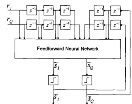
extent, then feeding the taps from the delay line into a static feedforward network. Thus, the channel inverse is achieved by training the static feedforward network. This can be referred to as inverse system identification. The basic configuration for achieving this is shown schematically in Fig. 3. The feedforward neural network-based decision feedback equalizer is placed behind the channel and receives both the channel outputs and detected symbols as its inputs. The network inputs at time k can be represented by X k = [ r z ,
s;]’,
where r k = [ r T ( k ) , . . . , r T ( k - n f ) l T ands k = [ S T ( k - l ) ,
.
. .,
s T ( k - 7 1 b ) l T . Notice that the receivedcomplex-valued signals r ( k ) should be represented by a 2 x 1 vector, i.e., [ T I , T Q ] ~ , because the error back-propagation algorithms cannot be applied to the complex-valued inputs directly, where T I and TQ represent the in-phase (real) and quadrature (imaginary) components of T ( IC). The detected symbols s ( k ) are generated by feeding the static neural
network outputs S ( k ) through a hardlimiter at time instant
k and given by S ( k ) = sign(s(k)), where S ( k ) = ”(ski w )
and sign(v) = [sign(v,), sign(v2), . . .
,
sZgn(v,)lT, ‘U =[ V I , v2, .
. .
,
v,IT. According to Fig. 3, the input-output relationship of the neural equalizer can be characterized by the function’
S ( k ) = NNDFE(zk; w ) = sign(NN(zr,; w ) ) (8) to-one mapping. Reference 141 showed that the best choice
for the code assignment is the Ungerboeck code for PSK signal in coded modulation. For example, the 8-PSK signal lo- cations (1,
o),
(-fi/2, fi/2), and(-fila,
- f i / 2 ) may be assigned to [-1, -1, -1IT, [-1, 1, -llT, and [l, 1, 1IT which correspond to the decimal representations “0,” “3,” and “5,” respectively. Generally, the bipolar representation can be extended to any other M-ary systems, i.e., QAM, GMSK, and CPM.Equation (6) becomes a weighted linear sum of transmitted symbols s(k)’s when the satellite channel does not include the nonlinear TWT amplifier. Thus, the transfer function of the satellite channel between the transmitter and receiver is denoted as H ( z ) , which is an FIR system. Widrow 1111
where w is the weight vector of the feedforward network and S ( k ) is the estimate of s ( k ) . The training data involved in transmitted symbols provide the desired response of the static feedforward network, dk(= s ( k ) ) to train the network to approximate the perfect channel inverse or ideal equalizer EOideal(.). Notice that a replica of the desired response is stored in the receiver. By the Stone-Weierstrass theorem, it is possible to find the appropriate weight vector w * of the static feedforward network of the neural-based equalizer, such that
(9) II”(2k; W * ) - EQideai(Zk))IXk
<
Efor an arbitrary t
>
0 and all the x k are in the region of interest.320 IEEE JOURNAL ON SELECTED AREAS IN COMMUNICATIONS, VOL. 13, NO. 2, FEBRUARY 1995
Feedforward Neural Network
Fig. 3. PSK system.
Architecture of neural-based decision feedback equalizer for .Wq
Since d k is represented by a bipolar-state vector, each
component of NN(zk; w * ) becomes either -1 or 1 after a sufficiently long training period. This would imply that NNDFE(zk; w * ) = "(zk; w * ) . From (9), we have
II"DFE(zk; w * ) - E Q I d e a i ( z k ) l l z k
<
6. (10)For an M-ary PSK signaling communication system, s(k),
;(IC), and S ( k ) should be represented by log, M x 1 vectors. Moreover, the received signal r ( k ) is complex-valued and then
can be expressed as a two-dimensional vector. Thus, the input layer of the network consists of two nf-tap forward filters, and log, M nb-tap feedback filters. As a result, the number of neurons in the input layer is given by
nZ = 2 x (nf f 1)
+
(log, M ) x n b . (11) In the output layer, the number of neurons is no = log, M .IV. MULTILAYER NEURAL NETWORKS AND THEIR LEARNING RULES
An iterative learning algorithm, called back propagation, was suggested by Rumelhart et al. [ 121. This iterative learning algorithm is used to adjust the weights and threshold levels of the network in a pattern-wise manner. In a mathematical sense, the back-propagation learning rule is used to train the feedforward network " ( E , w ) to approximate a function
f(z) from compact subset
D
of n,-dimensional Euclideanspace to a bounded subset
f( D )
of no-dimensional Euclidean space. Let Z k which belongs to D be the lcth pattern or sampleand selected randomly as the input of the neural network at time instant
k,
let " ( z k , w ) (= O k ) be the output of the neural network, and let f ( z k ) (= d k ) which also belongs to f ( D ) be the desired output. This task is to adjust all thevariable weights of the neural network such that the pattern- wise quadratic error E k can be reduced, where E k is defined
as
1 1 no
E k = -II"(zk, W ) - f ( z k ) 1 l 2 =
j
c
( o k , - d k , ) , (12)where no is the number of output nodes, Ok, and d k , are the
j t h components of Ok and d k , respectively. ,=1 2
Here, we define the weighted sum of the output of the previous layer by the presentation of input pattern z k
where w,, is the weight which connects the output of the ith neuron in the previous layer with respect to the j t h neuron, and
Okz is the output of the ith neuron. It should be noted that Okz is
equal to X k z when the ith neuron is located in the input layer,
where x k , is the ith component of pattern z k . Notice that the threshold level variables are treated as the additional weight variables in the network. Using ( 3 ) , the output of neuron j is
f x k ? 1
(14) if the neuron j belongs to the input layer
o k j =
{
G i n e t k j ) ,otherwise.
The pattern-wise or on-line back-propagation algorithm [ 121 minimizes the quadratic error E k by recursively altering the connection weight vector at each pattern according to the expression
where the learning rate q is usually set to be equal to a positive constant less than unity.
It is useful to see the partial derivative for pattern k ,
d E k / d w j , , as resulting from the product of two parts: one
part reflecting the change in error to a function of the change in the network input to the neuron, and one part representing the effect of changing a particular weight on the network input (16)
d E k - d E k d n e t k ,
dw3, d n e t k , dwJ2 '
From (13), the second part becomes
An error signal term I5 called delta produced by the j t h neuron is defined as follows
Note that E is a composite function of n e t k , , it can be
expressed as follows
E k = E k ( o k 1 , o k 2 , " ' , 0 k L )
= E k ( G ( n e t k i ) , G ( n e t k 2 ) , . . .
,
G ( n e t k L ) ) (19)where L is the number of the neurons in the current layer.
Thus, we have from (18)
Denoting the second term in (20) as a derivative of the activation function
CHANG AND WANG: ADAFTIVE DECISION FEEDBACK EQUALIZATION 32 1 However, to compute the first term, there are two cases. For
the hidden-to-output connections, it follows the definition of
E k that
Substituting for the two terms in (20), we can get
6 k j = ( d k j - O k j ) G ’ ( n e t k j ) . (23)
Second, for hidden (or input)-to-hidden connection, the chain rule is used to write
Substituting into (20), it yields
1
Equations (23) and (25) give a recursive procedure for computing the 6’s for all neurons in the network. In summary, the error signals 6’s for all neurons in the network can be computed according to the following recursive procedure
(26) if neuron j belongs to the output layer
{
G ’ ( n e t k j ) C l 6 k l w l j > 6 k j =otherwise.
It should be mentioned that O k i is equal to X k i when neuron
i belongs to the input layer. The expression of (26) is also called the generalized delta learning rule. Once those error signal terms have been determined, the partial derivatives for the quadratic error of the Icth pattern can be computed directly by
Thus, the update rule of the on-line back-propagation algo- rithm is
w j i ( k f 1) = w j i ( k )
+
7 6 k j o k i . (28)In the traditional equalizer, a replica of the desired response is stored in the receiver. Naturally, the generator of this stored reference has to be electronically synchronized with the known transmitted sequence. A widely used training signal consists of a pseudonoise (PN) sequence of length N B . Moreover,
the training signal can also be expressed as a collection of input-output data pairs, { Z k , d k } F & . The weights of neural-
based equalizer are updated by using the batch of these data pairs. Thus, the objective function should be modified in an expression of summation, E =
~~~,
E k , during the initial training. Thus, the update rule becomesNotice that the quantity w(Ic
+
1) is the updated weight vector after one pattern of learning; wneW is the updated weight vector after one batch of learning.It is shown that the batch back-propagation learning al- gorithm is used to initialize the weight coefficients of the neural-based equalizer when the channel is unknown. Nev- ertheless, the on-line learning algorithm is used to adjust the weights to track channel time variations and said to be decision directed. However, from [ 131, the initial training can be executed by the on-line learning algorithm instead of batch learning since on-line learning is shown to approach batch learning provided that 7 is small. Initialization may be aided by the transmission of N B known training symbols.
The trained neural-based equalizer converges to the channel inverse when N B is sufficiently large. It is known that the decision errors in equalizer tracking can lead directly to crashing of the equalizer, especially when the adaptation gain is high. Decision errors become more prevalent when the received signal-to-noise ratio is low, a condition that occurs unpredictably in nonlinear digital satellite channels. The susceptibility of adaptive equalizers or neural-based equalizers to crashes caused by propagation of decision errors implies that retraining procedures must be specific. For nonlinear satellite channel, periodic retraining is often used to improve reliability at some cost in throughput efficiency, via periodic insertion of training symbols into the data stream. More details about the packet adaptive equalization will be discussed in the next section.
A. Learning for Packet Adaptive Equalization
Packet equalization is a method that arises in TDMA communication systems, in which data are transmitted in fixed- length packets, rather than continuously [18]. It is usually assumed that the packet is largely self-contained for error detection, i.e., in terms of equalize initialization and at least fine synchronization. This overhead can achieve good perfor- mance with reasonable complexity. Packet equalization has some similarities with block-oriented methods for periodic training on continuous channels, although it is assumed that the channel state is independent from packet to packet. Frequency and packet synchronization are assumed to be maintained once initialized, but symbol timing and phase synchronization are assumed to be maintained once initialized, but symbol timing and phase synchronization typically need to be restored for each packet. It is known that the optimum approach to equalization is an off-line noncausal batch processing of the received signal with a large amount of training data. Such a formulation would be unfeasible and too complex to implement, but iterative approaches based on periodic training are possible. We will show that there is an equivalence of the off-line equalization and the packet-wise neural-based equalizer when the number of packets approaches infinity.
Considering the packet transmission, it is assumed that the length of the training data contained in the packet header and the total packet length are nu and n p , respectively. The main idea of the packet training scheme is used to train the neural- based equalizer with nu training data for each packet. The neural-based equalizer can be retrained for every packet and thus track the time variations in the channel. This is quite similar to the on-line training for a .sequence of packets.
322 IEEE JOURNAL ON SELECTED AREAS IN COMMUNICATIONS, VOL. 13, NO. 2. FEBRUARY 1995
The packet version of the back-propagation-based algorithm can be obtained by modifying (29) and given by
n,,
k = l
Furthermore, during data transmission after packet training period, the decision-directed adaptation is executed by (28). Similarly, the delta-bar-delta rule shown in the next section can also be applied to packet-wise back-propagation algorithm in order to increase the rate of convergence.
Furthermore, from the Stone-Weierstrass theorem, the exact channel inverse can be obtained by the batch learning when the length of training data is large enough and the maximum lags in both input and output of channel inverse are known. Espe- cially, for time-varying channels, N B would approach infinity.
But it is unfeasible for any channel equalizer transmitting a large amount of training data continuously. Fortunately, [ 171 shows that the problem is solved by inserting a finite number of training data into the data stream periodically. This leads to the following theorem.
Theorem 1: The neural equalizer is guaranteed to be capa- ble of converging to the channel inverse globally by perform- ing the packet back propagation algorithms with a sufficient number of hidden nodes when the maximum lags in the input and output of channel inverse are known. From [17] and the Stone-Weierstrass theorem, a solution w* can be generated by the packet-wise back-propagation algorithm such that
II"DFE(zk; U*) - EQideal(zk)IIzk
<
6 (31) for an arbitrary E>
0, as N -+ 30, where N is the numberof packets and N g = N
.
nu. B. Fast Learning AlgorithmsAlthough the back-propagation algorithm is a useful method to find an optimal solution of a set of weight values of a network, many researchers [ 141 showed that the convergence rate of this algorithm is relatively slow. It is necessary to find a faster algorithm to improve the back-propagation algorithm and also to achieve better performance. In this subsection, a modified back-propagation algorithm with much faster con- vergence rate will be introduced to the neural equalizer. This faster algorithm is used to modify the negative gradient direction by adjusting the learning rate, and it is called the delta-bar-delta rule [ 141.
Since a large 71 corresponds to rapid learning but might also result in oscillations, [12] suggests that expression (15) might be modified to include a sort of momentum term in order to dampen oscillation. That is, the weight u t j i is updated at the
k+lst iteration, according to the rule
where A w j i ( k
+
1) is the weight increment for the k+
1st iteration, ~ ( k+
1) is the learning rate value corresponding to A w ( k+
1) at time k+
1, and Q is the momentum rate.However, Jacobs [ 141 showed that the momentum can cause the weight to be adjusted up the slope of the system error
surface. This would decrease the performance of the learning algorithm. To overcome this difficulty, Jacobs [ 141 proposed a promising weight update algorithm based on the delta-bar- delta rule which consists of both a weight update rule and a learning rate update rule. The weight update rule is the same as the steepest descent algorithm and is given by ( 3 2 ) . The
delta-bar-delta learning rate update rule is described to follows
(6:
otherwisewhere X ( t ) = d E k / d w t J and x ( t ) = (1 - 6 ' ) A ( t )
+
B X ( t - 1).In these equations, X ( k ) is the partial derivative of the system error with respect wzJ at the kth iteration, and X ( k )
is an exponential average of the current and past derivatives with 6' as the base and index of iteration as the exponent. If the current derivative of a weight and the exponential average of the weight's previous derivatives possess the same sign, then the learning rate for that weight is incremented by a constant K . The learning rate is decremented by a proportion
4
of its current value when the current derivative of a weight and the exponential average of the weight's previous derivatives possess opposite signs.From ( 3 3 ) , it can be found that the learning rates of the delta-
bar-delta algorithm are incremented linearly in order to prevent them from becoming too large too fast. The algorithm also decrements the learning rates exponentially. This ensures that the rates are always positive and allows them to be decreased rapidly. Jacobs [14] showed that a combination of the delta- bar-delta rule and momentum heuristics can achieve both the good performance and faster rate of convergence.
More recent work has produced improved learning strategies based on extended Kalman algorithm [ 151 and a recursive pre- diction error routine [ 161. Although these two algorithms were each derived independently based on a different approach, they are actually equivalent. They both use the same search direc- tion called the Gauss-Newton direction, for which the negative gradient is multiplied by the inverse of an approximate Hessian matrix of the given criterion. The computational complexity of both algorithms applied to the neural equalizer is examined in [17].
ifX(k - 1)X(k)
>
o
A ~ ( J C
+
1) = -4q(Ic), ifX(k - I ) X ( ~ )<
o
( 3 3 )V. SIMULATION RESULTS
The QPSK satellite channel model used in performance evaluation is based on the Volterra series expansion model developed as a result of measurement [I], [2]. The associated Volterra series coefficients are shown in Table I. Moreover, the channel output is corrupted by zero mean additive white Gaussian noise (AWGN). For convenience, the received signal could be normalized to unity. Then the received signal-to-noise ratio (SNR) becomes the reciprocal of the noise variance at the input of the equalizer. The bit error rates were determined by simulating the QPSK data transmission system and taking an average of 100 individual runs of lo5 samples.
The complex-valued data are transmitted at a bit rate of 60 Mb/s over the Volterra-series-based QPSK satellite channel. The modulation scheme is QPSK with a symbol rate of 30
CHANG AND WANG: ADAmIVE DECISION FEEDBACK EQUALIZATION 1 0 , 323 ” ” I 0 10 20 30 40 SO 60 70 80 90 100 Number of packets Fig. 4.
DFE when R , = 40 and SNR = 10 dB.
Comparison of mean equare errors achieved by NNDFE and LMS-
M symbolsk and a symbol interval of 100 ns. The packet
length is set to 400 symbols (800 bits). A 10% overhead
would allow a maximum of 40 symbols for training, i.e.,
nu = 40. The neural-based decision feedback equalizer in- cludes a four-layer feedforward neural network. For simplicity, the neural equalizer is denoted by a short-hand notation NNDFE((nf, n b ) , n1, n2, no), where n f is the number of
forward taps, nb is the number of forward taps, n1 is the number of neurons in hidden layer 1 , n2 is the number of
neurons in hidden layer 2, and no is the number of neurons
in output layer. Similarly, traditional LMS decision feedback equalizer is denoted by LMSDFE ( n f
,
nb). According to thesuggestions of [3] and ( 1 l), n f and n b are set to be 3 and
2, respectively. Karam and Sari [3] showed that a two-stage
feedback filter can cancel most third- and higher-order IS1 terms resulted from the Volterra-series-based channel model. As discussed in Section 11-A, ni and no can be found as 12
and 2, respectively, for QPSK system. According to Huang
and Huang’s [lo] suggestions, it is possible to estimate the
lower bounds on the numbers of neurons in both hidden layers. Thus, n1 and 122 can be chosen as 20 and 10, respectively.
Fig. 4 illustrates MSE (mean square error) convergence of the packet-wise neural equalizer, NNDFE ((3, 2), 20, 10, 2 ) , and
LMSDEF(3, 2 ) with the same initial learning rate Q ( k ) l k = O
0.03 for training mode and 0.005 for decision-directed mode. The MSE is defined as follows
where S ( k ) = NNDFE(zk, w ) , N g = N
.
nu and dk denotesthe desired response. The values of parameters related to the delta-bar-delta rule are a = 0.8, K = 0.00005,
4
= 0.4, and 6’ = 0.3. The NNDFE requires at least 50 packets to converge, while the LMSDFE converges in about 8 packets. The results also show that the steady-state value of averaged square error produced by the NNDFE converges to a value( 5
-70 dB), which is much lower than the additive noise (-10 a: W
m
0 2 4 6 8 10 12 14 16 18 20
SNR (dB)
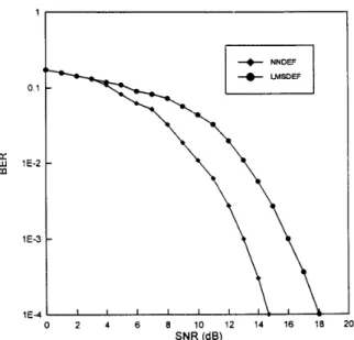
Comparison of bit error rates achieved by NNDFE and LMSDFE Fig. 5.
when nu = 40.
dB). This is a result of the approximation capability of packet back-propagation. Theorem 1 indicates that the approximation error approaches zero when the number of packets approaches infinity. The LMSDFE gives a steady value of averaged squared error at about -10 dB, which is around the noise floor.
Fig. 5 compares the respective bit error rates (BER’s) achieved by NNDFE ((3, 2), 20, 10, 2) and LMSDFE (3, 2). It may be
observed from Fig. 5 that the NNDFE attains about 3.2 dB improvement at BER = lop4 relative to the LMSDFE having the same number of input samples.
VI. CONCLUSION
This paper has introduced a four-layer neural-based adaptive decision feedback equalizer based on a concept of splitting which is capable of dealing with the M-ary PSK signals
over the complex digital satellite channel by using cost- effective real-valued training algorithms, where the real and imaginary components of neuron outputs are separately prop- agated back through the split complex activation function and its derivative. The neural-based DFE offers a superior performance as a channel equalizer to that of the conventional LMS DFE, because of its ability to approximate arbitrary nonlinear mapping. For comparison of simulation results for the Volterra-series-based QPSK satellite channel, it can be seen that the neural-based DFE provides better BER performance, especially in high-noise conditions; also, the MSE of neural- based DFE converges to a value which is much lower than that of LMS DFE after receiving a sufficient number of packets. These results would be conducted to verify the performance and approximation capability of packet-wise back propagation.
REFERENCES
[ I ] S. Benedetto, E. Biglien, and R. Daffara, “Modeling and evaluation of nonlinear satellite links-A Volttera series approach,” IEEE Trans. Aerosp. Electron. Syst., vol. AES-15, pp. 494-506, July 1979.
324 IEEE JOURNAL (
[2] S. Benedetto and E. Biglieri, “Nonlinear equalization of digital satellite channels.” IEEE Trans. J. Select. Areas Commun., vol. SAC-I, pp.
57-62, Jan. 1983.
[3] G. Karam and H. Sari, “Analysis of predistortion, equalization, and IS1 cancellation techniques in digital radio systems with nonlinear transmit amplifiers,” IEEE Trans. Commun., vol. 37, pp. 1245-1253, Dec. 1989.
[4] E. Biglien et al., Introduction to a Trellis-Coded Modulation with
Applications. New York: Macmillan, 1992.
[SI S. Siu, G. J. Gibson, and C. F. N. Cowan, “Decision feedback equaliza- tion using neural network structures and performance comparison with standard architecture.” IEEE Proc., vol. 137, pt. I, no. 4, pp. 221-225, Aug. 1990.
[6] S. Chen et al., “Adaptive equalization of finite nonlinear channels using multilayer perceprons,” Signal Processing, vol. 20, pp. 107-1 19, 1990. [7] M. E. Cotter, “The Stone-Weierstrass theorem and its application to neural nets,” IEEE Trans. Neural Networks, vol. 1, pp. 29&295, 1990. [8] G. Cybenko, “Approximations by superposition of a sigmoidal func-
tion,” Math. Contr. Syst. Signals, vol. 2, no. 4, 1989.
[9] D. Chester, “Why two hidden layers are better than one,” in Proc.
Int. Joint Con$ Neural Networks (Washington, DC), June 1989, pp. 1-6 1 3-1-6 18.
[IO] S. C. Huang and Y. F. Huang, “Bounds on the number of hidden neurons in multilayer perceptrons,” IEEE Trans. Neural Networks, vol. 2, pp. 47-55, Jan. 1991.
[ I l l B. Widrow and R. Winter, “Neural nets for adaptive filtering and adaptive pattern recognition,” IEEE Compur. Mag., vol. 21, pp. 25-39, Mar. 1988.
[I21 D. E. Rumelhart, G. E. Hinton, and R. J. Williams, “Learning internal representation by error propagation,” in Parallel Distributed Processing:
Explorations in the Microstructure of Congnition, vol. 1. Cambridge, MA: MIT Press, 1986, ch. 8.
[I31 S. Z. Qin, H. T. Su, and T. J. McAvoy, “Comparison of four neural net learning methods for dynamic system identification,” IEEE Trans.
Neural Networks, vol. 3 , pp. 122-130, Jan. 1992.
[I41 R. A. Jacobs, “Increased rates of convergence through learning rate adaption,” Neural Networks, vol. 1, pp. 295-307, 1988.
[IS] Y. Inguni, H. Sakai, and H. Tokumaru, “A real-time learning algorithm for a multilayered neural network based on the extended Kalman filter,”
IEEE Trans. Signal Processing, vol. 40, pp. 959-966, Apr. 1992. [16] S. Chen et al., “Parallel recursive prediction error algorithm for training
layered neural networks,” Int. J . Contr., vol. 51, no. 6, pp. 1215-1228,
1990.
[I71 P. R. Chang and C. C. Chang, “Adaptive packet equalization for indoor radio channel using multilayer neural networks,” IEEE Trans. Veh.
Technol., vol. 43, Aug. 1994.
IN SELECTED AREAS IN COMMUNICATIONS, VOL. 13, NO. 2, FEBRUARY 1995
[I81 J. G. Proakis, “Adaptive equalization for TDMA digital mobile radio,”
IEEE Trans. Veh. Technol., vol. 40, pp. 333-341, May 1991. [I91 D. L. Birx and S. J. Pipenberg, “A complex mapping network for
phase sensitive classification,” IEEE Trans. Neural Networks., vol. 4, pp, 127-135. Jan. 1993.
[2O] H. h u n g and S. Haykin, “The complex backpropagation algorithm,”
IEEE Trans. Signal Processing, vol. 39, no. 9, pp. 2101-2104, Sept. 1991.
Po-Rong Chang (M’87) received the B.S. degree in electrical engineering from the National Tsing- Hua University, Taiwan, in 1980; the M.S. degree in telecommunication engineering from National Chiao-Tung University, Hsinchu, Taiwan, in 1982; and the Ph.D. degree in electrical engineering from h r d u e University, West Lafayette, IN, 1988.
From 1982 to 1984 he was a Lecturer in the Chinese AN Force Telecommunication and Elec- tronics School for his two-year rmlitary service. From 1984 to 1985 he was an Instructor of electrical engineenng at National Taiwan Institute of Technology, Taipei, Taiwan. From 1989 to 1990 he was a Project Leader in charge of SPARC chip design team at ERSO of Industrial Technology and Research Institute, Chu-Tung, Taiwan. Currently he is an Associate Professor of Communication Engineering at National Chiao-Tung University. His current interests include fuzzy neural network, wireless multimedia systems, and virtual reality.
Bor-Chin Wang was born in Tainan, Taiwan, in 1961. He received the B.S. and M.S. degrees in power mechanical engineering from the National Tsing-Hua University, Hsinchu, Taiwan, in 1983 and 1985, respectively. He is presently working toward the Ph.D. degree in communication engineering at National Chiao-Tung University, Hsinchu, Taiwan.
From 1985 to 1993 he was an Assistant Research Engineer at the Chung-Shan Institute of Science and Technology, Ministry of National Defense, Republic of China, where he worked on servo system de- sign. His current research interests are in CDMA cellular system, wireless multimedia system, fuzzy neural network, and F‘CS systems.