應用於混模電路測試之利用混合基底與內插法的快速傅立葉轉換

全文

(1)國立交通大學電子工程學系. 電子研究所碩士班. 碩士論文應用於混模電路測試之利用混合基底與內插法的快速傅立葉轉換 FFT Based on Mixed-Radix and Interpolation for Mixed-Signal Testing 研究生: 陳見明指導教授: 李崇仁博士. 中華民國. 九十四年. 六. 月.

(2) 應用於混模電路測試之利用混合基底與內插法的快速傅立葉轉換 FFT Based on Mixed-Radix and Interpolation for Mixed-Signal Testing. 研究生：陳見明. Student: Jian-Ming Chen. 指導教授：李崇仁博士. Advisor: Dr. Chung-Len Lee. 國立交通大學電子工程學系電子研究所碩士班碩士論文 A Thesis Submitted to Department of Electronics Engineering & Institute of Electronics College of Electrical Engineering and Computer Science National Chiao Tung University in partial Fulfillment of the Requirements for the Degree of Master in Electronic Engineering June 2005 Hsinchu, Taiwan, Republic of China. 中華民國. 九十四年. 六. 月.

(3) 應用於混模電路測試之利用混合基底與內插法的快速傅立葉轉換研究生:陳見明. 指導教授:李崇仁博士. 國立交通大學電子工程學系電子研究所碩士班摘. 要. 在混模電路測試上，快速傅立葉轉換被廣泛地用來將時域訊號轉成頻域訊號以取得待測電路的傳輸參數，例如頻率響應、相位響應及訊號雜音比等等。但是，轉換過程需要大量的運算並且受制於取樣點數必須是 2 的冪次方。在此論文中，吾人提出一個利用混合基底 2/4、3 及 5 的快速傅立葉轉換演算法以增加運算速度並且增加可應用的取樣點數為 2、3 及 5 的冪次組合，此外再透過對取樣數據作內插的方法將取樣點數擴增為任意數。吾人先討論單一基底的快速傅立葉轉換，接著再將演算法擴充到混合基底。一個用來將取樣數據重新排列的演算法被找出來，這使得混合基底的快速傅立葉轉換可行。然後，吾人再將內插法的觀念與混合基底的快速傅立葉轉換結合，使混合基底的快速傅立葉轉換能操作在任意取樣點數。透過模擬，吾人從理論與實驗上對不同演算法作運算速度及取樣點數的比較。最後，吾人提出兩個實驗結果作為範例，一個是對多音訊號取樣，另一個是方波訊號。實驗結果顯示：在內插法造成訊號雜音比下降的可接受範圍內，演算法確實有速度上的優勢。. I.

(4) FFT Based on Mixed-Radix and Interpolation for Mixed-Signal Testing. Student: Jian-Ming Chen. Advisor: Dr. Chung-Len Lee. Department of Electronics Engineering & Institute of Electronics National Chiao Tung University. Abstract. In mixed-signal testing, FFT (fast Fourier transformation) is used widely to transform the time domain signal into the frequency domain signal to obtain the transmission parameters such as frequency response, phase response, signal to noise ratio (S/N), etc, for the circuit under test (CUT). However, the process is involved with large computation efforts and the limitation on the number of sampling points which need to be of the power of 2. In this thesis, we propose a FFT algorithm based on the mixed radixes of 2/4, 3 and 5 to increase the computation speed and to increase the applicable number of sampling points to the power of 2, 3 and 5, and furthermore to any number of sampling points by using an interpolation technique to interpolate the sampled data. We first discuss the single-radix FFT and then expand the algorithm to mixed-radix FFT. A re-ordering algorithm for the sampled data is found which makes the mixed-radix FFT possible. We then bring out the concept of II.

(5) interpolation to be in conjunction with the mixed-radix FFT to make the mixed-radix FFT algorithm be able to be applied to any number of sampling points. We compare the computation speed and the numbers of sampling points for different algorithms both theoretically and experimentally via simulation. Finally, experimental results on two examples, one is a multi-tone signal and the other is a square wave signal, are presented. They show that the algorithm can really demonstrate the speed advantage with acceptable degradation on S/N introduced by the interpolation process.. III.

(6) 誌. 謝. 首先，由衷地感謝指導教授李崇仁老師。由於老師的指導與鼓勵，我學習到研究的方法並一點一滴培養出認真的態度，這讓我能夠在研究上勇於面對難題，進而解決難題。研究之餘，老師則是和藹的長輩，與我分享人生經驗，我也因而得到啟發；或許我的未來仍是一片茫然，但是我學會從更多角度來思考事情，找尋人生的方向。其次，我也很感謝testing group的成員。竹一老師提供我許多寶貴的意見；明學學長、淑敏學姐及世平學長不厭其煩地為我解答問題；威憲、俊言、誌華及劉坪熱心地幫助我。這些協助使我能夠克服研究上及生活中的困難。另外，在交大的歲月裡，我的好哥兒們經緯及室友偉誠，也都提供我莫大的協助，令我相當感激。最後，深深感謝我摯愛的家人及親愛的女友，由於你們不斷地給予我支持和鼓勵，使得我能夠順利完成學業及研究。這篇論文，不僅僅是為我，同時也是為你們而作的。謹將本論文獻給你們，謝謝！. 陳見明謹誌於新竹交大九十四年. IV. 七月.

(7) Contents Chinese abstract. ..................................................................................................................Ⅰ. English abstract. ...................................................................................................................Ⅱ. Acknowledgments Contents. ...............................................................................................................Ⅳ. ...............................................................................................................................Ⅴ. List of Figures. ......................................................................................................................Ⅶ. List of Tables. ........................................................................................................................Ⅹ. Chapter 1. Chapter 2. Chapter 3. Introduction. ....................................................................................................1. 1.1. Motivation. ..............................................................................................1. 1.2. Review of Previous Works. 1.3. Outline of This Thesis. .....................................................................3. ............................................................................4. Single-Radix FFT ...........................................................................................5 2.1. Decimation-In-Time Algorithm .............................................................5. 2.2. L-point FFT ............................................................................................9 2.2.1. 3-point FFT .............................................................................10. 2.2.2. 4-point FFT ..............................................................................11. 2.2.3. 5-point FFT .............................................................................12. 2.3. Re-Ordering Algorithm for Input Sequence. .........................................14. 2.4. Speed Ratio of Radix-L FFT to Rarix-2 FFT .......................................15. 2.5. Numbers of Sampling Points ...............................................................16. Mixed-Radix FFT .........................................................................................18 3.1. Radix-A/B FFT .....................................................................................18 3.1.1. Decimation-In-Time Algorithm ..............................................18. 3.1.2. Re-Ordering Algorithm for Input Sequence V. ............................20.

(8) 3.2. Chapter 4. Chapter 5 References Vita. Radix-A/B/C FFT .................................................................................22 3.2.1. Decimation-In-time Algorithm ................................................22. 3.2.2. Re-Ordering Algorithm for Input Sequence. Radix-2/4/3/5 FFT and Interpolation. ............................24. .........................................................25. 4.1. Radix-2/4/3/5 FFT Algorithm. 4.2. Interpolation Algorithm ........................................................................26. 4.3. Simulation Results. 4.4. Examples. ...............................................................................27. ..............................................................................................34. 4.4.1. Multi-tone Signal. 4.4.2. Square Wave. Conclusion. ..............................................................25. ....................................................................34. ............................................................................39. ....................................................................................................44. ............................................................................................................................45. .......................................................................................................................................47. VI.

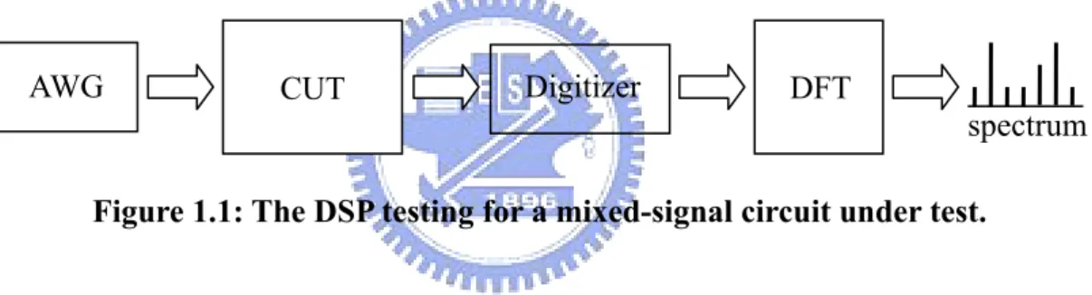
(9) List of Figures Figure 1.1. The DSP testing for a mixed-signal circuit under test.. Figure 1.2. A comparison of computation complexity between DFT and FFT.. Figure 1.3. A method that combines interpolation with mixed-radix FFT. .........................3. Figure 2.1. The first step in the decimation-in-time algorithm.. Figure 2.2. The second step in the decimation-in-time algorithm.. Figure 2.3. The last step in the decimation-in-time algorithm.. Figure 2.4. The visual representation of the 3-point DFT.. Figure 2.5. The visual representation of the 3-point FFT (butterfly structure).. Figure 2.6. The visual representation of the 4-point DFT.. Figure 2.7. The visual representation of the 4-point FFT (butterfly structure). ................12. Figure 2.8. The visual representation of the 5-point DFT.. Figure 2.9. The visual representation of the 5-point FFT (butterfly structure). ................13. Figure 2.10. The process of re-ordering the input samples for radix-3 FFT.. Figure 2.11 9-point decimation-in-time FFT algorithm.. .....................................1 .................1. ..........................................7 .....................................8. ...........................................9. ................................................10 ................11. ................................................11. ................................................12. ......................14. ....................................................14. Figure 3.1. The radix-A/B FFT decimation.. ......................................................................19. Figure 3.2. The 6-point FFT computed by the radix-2/3 algorithm. .................................19. Figure 3.3. The 6-point FFT computed by the radix/3/2 algorithm.. Figure 3.4. The 6-point radix-2/3 re-ordering algorithm.. Figure 3.5. The Radix-A/B/C FFT decimation.. Figure 3.6. The 30-point FFT computed by the radix-2/3/5 algorithm.. Figure 3.7. The illustration of a 30-point radix-2/3/5 re-ordering algorithm.. Figure 4.1. The radix-2/4/3/5 FFT decimation. VII. .................................20. .................................................21. .................................................................22 ............................23 ...................24. .................................................................25.

(10) Figure 4.2. The 30-point radix-2/4/3/5 re-ordering algorithm.. .........................................26. Figure 4.3. The illustration of linear interpolation.. Figure 4.4. The flow chart of N-point FFT operated by the new algorithm.. Figure 4.5. The comparison of applicable number (Ni) of sampling points which can be applied by the single-radix FFT’s. .......................................................28. Figure 4.6. The comparison of applicable number (Ni) of sampling points which can be applied by the mixed-radix FFT’s. ......................................................29. Figure 4.7. The visual representation of ΔN (Ni - Ns) for different mixed-radix FFT’s.. Figure 4.8. The comparison of 1 - |ΔN/Ns| for different mixed-radix FFT’s. ...................30. Figure 4.9. The comparison of run-times of radix-2 FFT and radix-2/4 FFT.. Figure 4.10. The comparison of run-times of radix-2,3,5 FFT and radix-2/4,3,5 FFT.. ...........................................................27 ....................27. ..30. ..................31 ......32. Figure 4.11 The comparison of run-times of radix-2,3 FFT, radix-2,5 FFT and radix-2,3,5 FFT. ..............................................................................................33 Figure 4.12 The comparison of run-times of radix-2,3 FFT, radix-2,5 FFT and radix-2/4,3,5 FFT. ...........................................................................................33 Figure 4.13 The waveform of the multi-tone signal.. .........................................................34. Figure 4.14 The comparison of applicable number (Ni) of sampling points which can be applied by the FFT’s. ...........................................................................35 Figure 4.15. The comparison of run-times of different FFT algorithms.. ............................36. Figure 4.16 4.15: The comparisons of magnitudes of each tone of different FFT algorithms (a) 1st tone, (b) 2nd tone, (c) 3rd tone, and (d) 4th tone. ..................36 Figure 4.17 The comparison of magnitudes of signal of different FFT algorithms.. ..........37. Figure 4.18 The comparisons of magnitudes of noise of different FFT algorithms (a) with DFT value as a reference, and (b) without DFT value. .....................38 Figure 4.19 The comparisons of S/N’s of each tone of different FFT algorithms (a) 1st tone, (b) 2nd tone, (c) 3rd tone, and (d) 4th tone. ....................................39 Figure 4.20 The comparison of S/N’s of signal of different FFT algorithms. VIII. ...................39.

(11) Figure 4.21. The waveform of the square wave.. .................................................................40. Figure 4.22 The comparison of applicable number (Ni) of sampling points which can be applied by the FFT’s. ...........................................................................41 Figure 4.23. The comparison of run-times of different FFT algorithms.. ............................41. Figure 4.24 The comparison of magnitudes of signal of different FFT algorithms.. ..........42. Figure 4.25 The comparisons of magnitudes of noise of different FFT algorithms (a) with DFT value as a reference, and (b) without DFT value. .....................42 Figure 4.26 The comparison of S/N’s of signal of different FFT algorithms.. IX. ...................43.

(12) List of Tables Table 1.1. The numbers of sampling points which can be applied by the radix-2 FFT under the value 10000. ...............................................................................2. Table 2.1. The comparison of computation complexity of different FFT algorithms.. Table 2.2. The computation time of a butterfly structure for each algorithm. ..................16. Table 2.3. The speed ratio of radix-L FFT to radix-2 FFT.. Table 2.4. The numbers of sampling points which can be applied by the radix-3 FFT under the value 10000. .............................................................................17. Table 3.1. A comparison of the radix-A/B FFT and the radix-B/A FFT. ...........................21. X. ......13. ...............................................16.

(13) Chapter 1. Introduction. 1.1 Motivation Mixed-signal circuits are widely used in the present electronic system, especially, in SoC. To test mixed-signal circuits [1], Digital Signal Processing approach is usually adopted, which is shown in Figure 1.1. An appropriately selected test patterns are applied the mixed signal circuit under test (CUT) and its response is transformed into the frequency domain by using the discrete Fourier transform (DFT) technique. The transformed spectrum is analyzed to deduce the transmission parameters such as frequency response, S/N, etc, for the CUT. It can then analyze the obtained parameters by comparator to mark the CUT as good or faulty.. AWG. CUT. Digitizer. DFT spectrum. Figure 1.1: The DSP testing for a mixed-signal circuit under test. In the above, the DFT is a computation-intensive process which is proportional to N2, where N is the number of sample points of the output response of the CUT. In 1965, a much faster algorithm was developed by Cooley and Tukey [2], which is called the fast Fourier transform (FFT) algorithm [3]-[7]. The computation complexity for the algorithm (radix-2 FFT) is proportional to Nlog2N.. Figure 1.2: A comparison of computation complexity between DFT and FFT. 1.

(14) Figure 1.2 plots the comparison of computation complexity of the DFT and FFT algorithms. However, radix-2 FFT has an important limitation, that is, the number of sampling points must be of the power of 2, i.e., 2k, where k is a natural number. This means that the numbers of sampling points to be able to be applied by using the FFT algorithm are very limited. For example as shown in Table 1.1, for a sampling system which can hold 10000 data points, there are only 13 numbers of sampling points can be used the FFT.. k k. 2 distance. 1 2 -. 2 4 2. 3 8 4. 4 16 8. 5 32 16. 6 64 32. 7 128 64. 8 256 128. 9 512 256. 10 11 12 13 1024 2048 4096 8196 512 1024 2048 4096. Table 1.1: The numbers of sampling points which can be applied by the radix-2 FFT under the value 10000. In this thesis work, it is to investigate to apply the FFT algorithm to, in addition to the number of sampling points that is of radix 2, other numbers which could be of other radixes such as 3, 4, and 5 and a mixed of the above numbers. This will increase the range of application of FFT. In addition, to apply the FFT in a mixed-radix fashion may have a faster computation speed since its number of computation stages is fewer than that of the radix-2 FFT when their numbers of sampling points are similar. Furthermore, although mixed-radix FFT can increase the numbers of sampling, which can be applied by the FFT algorithm, significantly, the numbers are still too few. Hence we will investigate a technique to use interpolation to adjust the sampling points to be able to be applied the mixed-radix FFT, as shown in Figure 1.3, to further increase the FFT efficiency.. 2.

(15) sampled signal. mixed-radix FFT. interpolation adjust the number of sampling points. mixed-signal testing. transform the domain of signal. Figure 1.3: A method that combines interpolation with mixed-radix FFT. However, by using the interpolation to the number of sampling points to match up the mixed-radix FFT, we will introduce errors to the final computation results, which are expressed in worse S/N’s. When the distribution of the numbers of sampling points is even enough, the difference between the original number and the interpolated number will be small. However, this will usually lead to a more complicated mixed-radix FFT. So we will study the trade-off between the decreased S/N and the increased computation complexity.. 1.2. Review of Previous Works. To speed up the FFT operation, there were several algorithms proposed. An FFT using radix-3, 6, and 12 algorithms was used in an ordinary complex plane and the numbers of additions and multiplications were shown to have significantly reduced [8]. Radix-2/8 FFT algorithm was also demonstrated to be able to save real multiplications and have much lower arithmetic complexity than the radix-2/4 FFT algorithm [9]. The form of radix-p/p2 algorithm is called a split-radix algorithm, which is better than radix-p algorithm on length-pm DFT’s. It was shown that whenever a radix-p2 outperforms a radix-p algorithm, then a radix-p/p2 algorithm will outperform both of them [10][11]. As to the limitation of numbers of sampling points, there were two algorithms that can do the FFT for any number of sampling points [12][13]. The proposed algorithms can flexibly compute the discrete Fourier transforms of length q×2m where q is an odd integer. Comparisons with previously reported algorithms show that substantial savings on arithmetic operations can be made. Furthermore, a wider range of 3.

(16) choices on different sequence lengths is naturally provided. In this thesis, we propose a mixed radixes FFT based on mixed radixes 2/4,3,5 incorporating with an interpolation technique to speed up the FFT while still maintaining a good S/N.. 1.3 Outline of This Thesis This thesis is organized as follows. Chapter 2 presents the research on single-radix FFT. Chapter 3 presents the research on mixed-radix FFT. Chapter 4 presents the radix-2/4/3/5 FFT and interpolation. In chapter 5, conclusions are given.. 4.

(17) Chapter 2. Single-Radix FFT. Before deriving the mixed-radix FFT algorithm, we first study the single-radix FFT algorithm. We first study the decimation-in-time algorithm for the general case and then apply it to radix-3 FFT, radix-4 FFT and radix-5 FFT. As for the radix-2 FFT [6][7], since it is well known in the general literature, we will not mention it here in detail.. 2.1 Decimation-In-Time Algorithm Decimation is the process of breaking down a group of data into several of its constituents. Decimation-in-time involves breaking down a signal which is a set of discrete time data into several smaller set of discrete time data which represent the same signal. Let us consider N (= LS)-point DFT where N is the number of total sampled data points, L is a decimating factor and S is the corresponding exponent. We split the N-point data sequence x(n) into L data sequences, f1(n), f2(n),..., fL(n), with N/L points for each sequence. That is, f1 (n) = x( Ln) f 2 (n) = x( Ln + 1) M f L (n) = x( Ln + L − 1),. n = 0,1,..., N. L. −1. f1(n), f2(n),..., fL(n) are the decimated sub-sequences of x(n) by the factor L. Now the N-point DFT can be expressed in terms of the DFT’s of the decimated sub-sequences as follows:. 5.

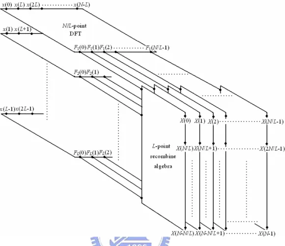
(18) N −1. X (k ) = ∑ x(n)WNkn ,. k = 0,1,..., N − 1. n=0. =. N L −1. ∑. m=0. x( Lm)WNLmk +. N L −1. ∑. m=0. x( Lm + 1)WN( Lm +1) k + L +. N L −1. ∑. m=0. x( Lm + L − 1)WN( Lm + L −1) k. Where WNL = WN/L. With this substitution, the equation can be expressed as. X (k ) =. N L −1. ∑. m =0. f1 (m)WNkmL + WNk. N L −1. ∑. m =0. f 2 (m)WNkmL + L + WN( L −1) k. ( L −1) k N. =F1 (k ) + W F2 (k ) + L + W k N. N L −1. ∑. m=0. f L (m)WNkmL. k = 0,1,..., N − 1. FL (k ),. Where F1(k), F2(k),…, FL(k) are the N/L-point DFT’s of the sequences f1(m), f2(m),…, fL(m), respectively. Since F1(k), F2(k),…, FL(k) are periodic with period N/L, we have F1(k+N/L) = F1(k), F2(k+N/L) = F2(k),…, FL(k+N/L) = FL(k). Hence the equation may be expressed as X (k ) = F1 (k ) + WNk F2 ( k ) + L + WN( L −1) k FL ( k ) 2π. −j −j X (k + N ) = F1 (k ) + e L WNk F2 (k ) + L + e L M −j X (k + ( L − 1) N ) = F1 (k ) + e L. ( L −1)⋅2π L. ( L −1)⋅2π L. WN( L −1) k FL (k ). W F2 (k ) + L + e k N. k = 0,1,..., N. L. −j. ( L −1)2 ⋅2π L. WN( L −1) k FL ( k ). −1. We can observe that the direct computation of F1(k) requires approx (N/L)2 complex multiplications. The same applies to other N/L-point DFT’s. Furthermore, there are (L-1)N additional complex multiplications required to compute other parts. Hence the entire computation of X(k) requires L(N/L)2 + (L-1)N = N 2/L + LN complex multiplications. The first step results in a reduction of the number of complex multiplications from approximate N 2. to N 2/L + LN, which is about a factor of L for a large N. This process of decimating the signal can easily be visualized. The first breakup into. 6.

(19) several N/L-point DFT’s can be shown as Figure 2.1.. Figure 2.1: The first step in the decimation-in-time algorithm.. We can continue to split the N/L-point data sequence fi(n) into L data sequences with N/L2 points for each sequence gi1(n), gi2(n),..., giL(n), that is, gi1 (n) = f i ( Ln) gi 2 (n) = fi ( Ln + 1) M gi L (n) = fi ( Ln + L − 1),. i = 1, 2,..., L;. n = 0,1,..., N. L2. −1. By computing N/L2-point DFT’s, we obtain the N/L-point DFT’s F1(k), F2(k),…, FL(k) from the relationship:. 7.

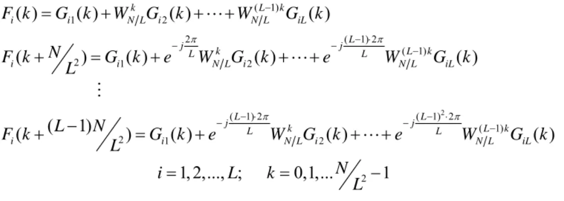
(20) Fi (k ) = Gi1 (k ) + WNk LGi 2 (k ) + L + WN( LL−1) k GiL (k ) F (k + N i. 2. L. ) = Gi1 (k ) + e. −j. 2π L. k N L. W. Gi 2 (k ) + L + e. −j. ( L −1)⋅2π L. WN( LL−1) k GiL (k ). M F (k + ( L − 1) N i. 2. L. ) = Gi1 (k ) + e. −j. ( L −1)⋅2π L. i = 1, 2,..., L;. k N L. W. Gi 2 (k ) + L + e. k = 0,1,... N. L2. −j. ( L −1)2 ⋅2π L. WN( LL−1) k GiL (k ). −1. The decimation process is taken another stage by breaking down the N/L-point DFT’s into N/L2-point DFT’s as shown in Figure 2.2.. Figure 2.2: The second step in the decimation-in-time algorithm.. The decimation of the data sequence can be repeated again and again until a series of L-point DFT’s as shown in Figure 2.3 is reached.. 8.

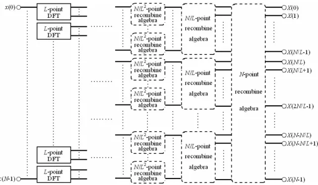
(21) Figure 2.3: The last step in the decimation-in-time algorithm.. Since each stage takes approx L2 × (N/L) = LN complex multiplications and there are logLN (= S) stages, the total number of complex multiplications is LNlogLN. This means that this decimation approach has reduced the number of complex multiplications from approx N2 to LNlogLN. In section 2.2 we will derive the L-point FFT which can reduce a little more complex multiplications and then replace the L-point DFT with the L-point FFT. Another important observation is on the order of the input sequence after it is decimated (S-1) times. For example, if we consider the case where N = 9 and L = 3, we know that the decimation yields the sequence in the order of: {x(0), x(3), x(6), x(1), x(4), x(7), x(2), x(5), x(8)}. An algorithm which can re-order the input data sequence will be discussed in section 2.3.. 2.2 L-point FFT We have derived the decimation-in-time algorithm which can reduce the amount of computation significantly for any single-radix FFT. But the decimated result is not the 9.

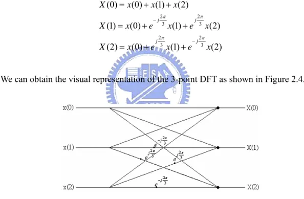
(22) simplest since the equation of the L-point DFT has conjugate pairs that can be simplified. Here we will show the process of deriving the 3-point FFT from the equation of the 3-point DFT as an example and then show the 4-point FFT and 5-point FFT. Finally, we will have a table to compare the amount of computation of these three algorithms with that of the radix-2 FFT.. 2.2.1 3-point FFT Let us consider the case of the 3-point DFT. According to equations: X (0) = x(0) + x(1) + x(2) X (1) = x(0) + e. −j. X (2) = x(0) + e. j. 2π 3. 2π 3. x(1) + e x(1) + e. j. 2π 3. −j. 2π 3. x(2) x(2). We can obtain the visual representation of the 3-point DFT as shown in Figure 2.4.. Figure 2.4: The visual representation of the 3-point DFT.. The 3-point DFT requires 4 complex multiplications and 6 complex additions. Thus if we consider the computation of the N3 (= 3S)-point DFT, the decimation approach will require (4N3/3)log3N3 complex multiplications and 2N3log3N3 complex additions. Let us pay attention to the equations of 3-point DFT, and then we can find that there are only two multiplications, exp(j2π/3) and exp(-j2π/3). Since these two complex values are conjugate, they have equal real-part and inverse imaginary-part. Hence we can rewrite the 10.

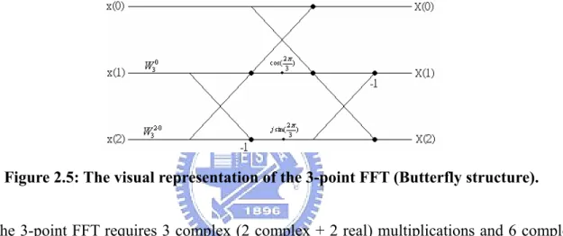
(23) equations as follows: X (0) = X (0) + W30 X (1) + W32⋅0 X (2) 2π 2π ) ⎡⎣W30 X (1) + W32⋅0 X (2) ⎤⎦ − j sin( ) ⎡⎣W30 X (1) − W32⋅0 X (2) ⎤⎦ 3 3 2π 2π X (2) = X (0) + cos( ) ⎡⎣W30 X (1) + W32⋅0 X (2) ⎤⎦ + j sin( ) ⎡⎣W30 X (1) − W32⋅0 X (2) ⎤⎦ 3 3 X (1) = X (0) + cos(. According to these new equations, we can obtain the visual representation of the 3-point FFT as shown in Figure 2.5. We call this a “Butterfly Structure” of the radix-3 FFT.. Figure 2.5: The visual representation of the 3-point FFT (Butterfly structure).. The 3-point FFT requires 3 complex (2 complex + 2 real) multiplications and 6 complex additions. Thus if we consider the computation of the N3-point FFT, the decimation approach will require N3log3N3 complex multiplications and 2N3log3N3 complex additions.. 2.2.2 4-point FFT We directly consider the visual representation of the 4-point DFT as shown in Figure 2.6.. Figure 2.6: The visual representation of the 4-point DFT.. 11.

(24) The 4-point DFT requires 9 complex multiplications and 12 complex additions. Thus if we consider the computation of the N4 (= 4S)-point DFT, the decimation approach will require (9N4/4)log4N4 complex multiplications and 3N4log4N4 complex additions. And then we consider the visual representation of the 4-point FFT as shown in Figure 2.7. We call this a “Butterfly Structure” of the radix-4 FFT.. Figure 2.7: The visual representation of the 4-point FFT (Butterfly Structure).. The 4-point FFT requires 3 complex multiplications and 8 complex additions, thus if we consider the computation of the N4-point FFT, the decimation approach will require (3N4/4)log4N4 complex multiplications and 2N4log4N4 complex additions.. 2.2.3 5-point FFT We directly give the visual representation of the 5-point DFT as shown in Figure 2.8.. Figure 2.8: The visual representation of the 5-point DFT.. The 5-point DFT requires 16 complex multiplications and 20 complex additions, thus if. 12.

(25) we consider the computation of the N5 (= 5S)-point DFT, the decimation approach will require (16N5/5)log5N5 complex multiplications and 4N5log5N5 complex additions. And then we give the “Butterfly Structure” of the 5-point FFT as shown in Figure 2.9.. Figure 2.9: The visual representation of the 5-point FFT (Butterfly Structure).. The 5-point FFT requires 8 complex (4 complex + 8 real) and 16 complex additions. Thus if we consider the computation of the N5-point FFT, the decimation approach will require (8N5/5)log5N5 complex multiplications and (16N5/5)log5N5 complex additions. Obviously, the number of complex multiplications is reduced again by replacing L-point DFT with L -point FFT. We have final comparison as shown in Table 2.1. algorithm complex multiplication complex addition. radix-2 FFT (N/2)log2N Nlog2N. radix-3 FFT Nlog3N 2Nlog3N. radix-4 FFT (3N/4)log4N 2Nlog4N. radix-5 FFT (8N/5)log5N (16N/5)log5N. Table 2.1: The comparison of computation complexity of different FFT algorithms.. Although radix-2 FFT has the minimum number of complex multiplication (N/2) for each stage, however other single-radix FFT’s have fewer number of computation stages. Thus other algorithms could have better performance in speed than radix-2 FFT in certain circumstances. This will be discussed further in section 2.4.. 2.3 Re-Ordering Algorithm for Input Sequence 13.

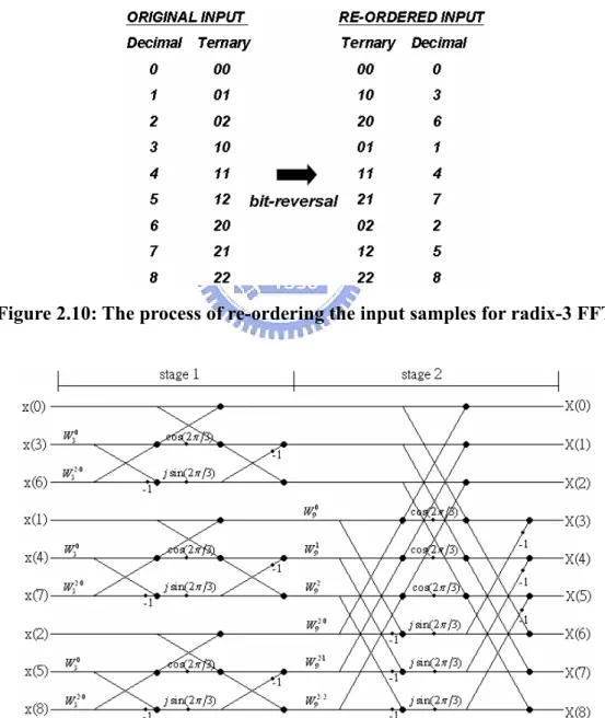
(26) The process of decimating the signal in the time domain has made input samples need to be re-ordered. For a 9-point signal, the original order of the samples is 0, 1, 2, 3, 4, 5, 6, 7 and 8. But after decimating by radix-3 FFT the order becomes 0, 3, 6, 1, 4, 7, 2, 5 and 8. The order can be obtained by representing the number in the ternary form as follows in Figure 2.10. In the figure, once the numbers are represented in the ternary form, the digits of the representing ternary bits are reversed. The new numbers represented by the reversed digits are the new sequence which is to be applied to the decimated FFT.. Figure 2.10: The process of re-ordering the input samples for radix-3 FFT.. Figure 2.11: 9-point decimation-in-time FFT algorithm.. 14.

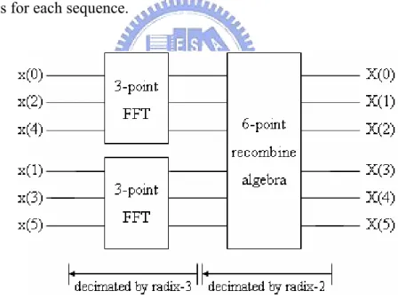
(27) For the illustrative purpose, we depict the computation of 9-point FFT in Figure 2.11. The computation is performed in two stages, beginning with the computations of three 3-point FFT’s, and finally one 9-point recombine algebra. As for the radix-4 FFT or radix-5 FFT, we can also apply the same bit-reversal procedure to re-order the in put sequence. In the process, we have to remember to first represent the numbers in the quaternary and quinary form respectively.. 2.4 Speed Ratio of Radix-L FFT to Radix-2 FFT In section 2.2, we have a table to compare the computation complexity of different single-radix FFT’s. In this section, however we will use the idea of butterfly structure to obtain the same result. We will count how many butterfly structures are used for an algorithm. We have an equation to obtain the amount of butterfly structures for each algorithm, that is, radix-L FFT: ( N L L) log L N L ,. N L is of the power of L L = 2, 3, 4, 5. Where NL/L is the number of butterfly structures at each stage and logLNL is the number of stages for an algorithm. The computation time of a butterfly structure (TL) is:. radix-L FFT:TL =. Trun total run-time = amount of butterfly structures ( N L L) log L N L. Because the computation time of the process of re-ordering is very small and can be ignored, so we can directly use the total run-time of the radix-L FFT to calculate TL. We use MATLAB to run the radix-L FFT, record the total run-time and the amount of butterfly structures for each algorithm, and then we can obtain TL for each algorithm as shown in Table 2.2.. 15.

(28) TL. T2. T3. T4. T5. us. 1.76. 2.59. 3.47. 4.69. Table 2.2: The computation time of a butterfly structure for each algorithm.. After obtaining TL for each algorithm, we can start to calculate the speed ratio. Let us assume the numbers of sampling points N2 is very close to N3, N4 and N5 in value, then according to the following equation, 1 1 Trun − L TL ( N L L) log L N L T2 × L = ≈ ⋅ log 2 L speed ratio (L to 2) = 1 1 TL × 2 Trun − 2 T2 ( N 2 2) log 2 N 2 when N 2 ≈ N L We can easily calculate the speed ratio of radix-L FFT to radix-2 FFT as shown in Table 2.3. algorithm speed ratio. radix-2 FFT 1. radix-3 FFT 1.02．log23. radix-4 FFT 1.01．log24. radix-5 FFT 0.94．log25. Table 2.3: The speed ratio of radix-L FFT to radix-2 FFT.. Obviously, the computation speed ratio of radix-L FFT to radix-2 FFT is very close to log2L which is larger than one. So, radix-3 FFT, radix-4 FFT and radix-5 FFT have a better performance than does the radix-2 FFT.. 2.5 Numbers of Sampling Points As discussed, radix-L FFT’s have a speed performance improvement over the radix-2 FFT, there is another issue which needs to be considered. That is the number of numbers of sampling points which can be applied by FFT’s. In the following, we will discuss this issue. For the radix-2 FFT, the number of sampling points which can be applied by the FFT must. 16.

(29) be a number equal to 2k, where k is a natural number. Similarly for the radix-3 FFT, the number of sampling points must be one of the series 3k. Table 2.4 lists the numbers of sampling points that can be applied by the radix-3 FFT under the value 10000. There are only 8 numbers of sampling points. This is fewer than that of the radix-2 FFT, which is 13. The higher radix FFT, the fewer this number. For radix-4 and radix-5 FFT, the number becomes 6 and 5 respectively. This is a drawback for using a higher radix FFT.. k k. 3 distance. 1 3 -. 2 9 6. 3 27 18. 4 81 54. 5 243 162. 6 729 486. 7 2187 1458. 8 6561 4374. Table 2.4: The numbers of sampling points which can be applied by the radix-3 FFT under the value 10000.. Chapter 3. Mixed-Radix FFT. 17.

(30) As we have discussed in the previous chapter, the FFT’s other than radix-2 have the advantages of speed improvement but have the drawback that the numbers of sampling points become less. A good solution for bypassing the drawback is that we can apply FFT’s for a set of sampling points by dividing the computation stages into several groups and apply the FFT of different radix for each group of computation stages. We call this the “mixed radix-FFT” algorithm. In this chapter, we will derive the mixed-radix FFT based on the results obtained in the previous chapter. First we will discuss the case of two radixes, i.e., radix-A/B FFT, and then the case of three radixes, i.e., radix-A/B/C FFT.. 3.1 Radix-A/B FFT Radix-A/B FFT has two factors A and B. According to the order of permutation of these two factors, there will be several forms of algorithm that can be used to decimate the data sequence. For example, if the data sequence has N (= A2×B) points, there will be three forms of permutation of A and B, i.e., AAB, ABA and BAA. We only consider the permutation AA…ABB…B since all other permutations can be applied the same analysis.. 3.1.1. Decimation-In-Time Algorithm. Let us consider the data sequence x(n) with N (= AmA×BmB ) sampling points. First we decimate the data sequence by a factor of A repeatedly until the data sequence is split into AmA data sequences of which each has BmB sampling points. And then we decimate each of these data sequences further by a factor of B repeatedly until these data sequences each is a series of B-point FFT’s. This process can be shown as in Figure 3.1.. 18.

(31) Figure 3.1: The radix-A/B FFT decimation.. In the figure, ‘mA-stage’ means the data sequence is decimated by the radix-A algorithm (mA-1) times, ‘mB-stage’ means the data sequences are decimated by the radix-B algorithm (mB-1) times, and ‘AmA-block and BmB-point’ means there are AmA data sequences with BmB sampling points for each sequence.. Figure 3.2: The 6-point FFT computed by the radix-2/3 algorithm.. For an example, Figure 3.2 depicts the 6-point FFT computed by the radix-2/3 algorithm which is stated above. We observe that the data sequence is finally decimated into two 3-point FFT’s. Besides using the radix-2/3 algorithm, we can also use the radix-3/2 algorithm to do the same 6-point FFT. For this case, the data sequence is finally decimated into three 2-point FFT’s as shown in Figure 3.3.. 19.

(32) Figure 3.3: The 6-point FFT computed by the radix-3/2 algorithm.. 3.1.2. Re-Ordering Algorithm for Input Sequence. The re-ordering algorithm used for the radix-A/B FFT is very different from that used for the single-radix FFT. Since there are two factors in the algorithm, the previous bit-reversal procedure can not be used directly. Here we consider the process of the decimation-in-time algorithm. We first use the radix-A to decimate the data sequence to reach several blocks. We observe the order of the data sequence in every block and try to find a mathematical relation to describe such result. And then we use the radix-B to decimate each block which has BmB sampling points. Before decimating, we re-assign numbers beginning from 0 to the data sequences in each block and record the true order and the new number of each data. After this, we use the bit-reversal (radix-B re-ordering) procedure to re-order the data in each block. Finally, we can obtain the input order according to the previous record. However the above method is a little bit complicated. We can directly find a mathematical relation to describe the input order. The following Figure 3.4 depicts the 6-point radix-2/3 re-ordering algorithm. This algorithm can be extended to radix-A/B.. 20.

(33) Figure 3.4: The 6-point radix-2/3 re-ordering algorithm.. In the figure, ‘0, 1, 2, 3, 4, 5’ means the original order, ‘0, 2, 4, 1, 3, 5’ means the decimated order and the part written on the right of the equal sign is the re-ordering algorithm. ‘N1-point radix-2 re-ordering’ means using bit-reversal (radix-2 re-ordering) to re-order the sequence of numbers 0…N1-1 where N1 is of the power of 2. ‘(N2-point radix-3 re-ordering) × N1’ means using bit-reversal (radix-3 re-ordering) to re-order the sequence of numbers 0…N2-1 where N2 is of the power of 3, and then multiplied by the sequence N1. One thing to be noted is that: For applying the radix-A/B FFT or the radix-B/A FFT, the order of A and B will give different run-time. Table 3.1 compares the computation speed for the radix-A/B FFT and the radix-B/A FFT under the different conditions.. AmA ＞ BmB. BmB ＞ AmA. radix-A/B FFT. slow. fast. radix-B/A FFT. fast. slow. Table 3.1: A comparison of the radix-A/B FFT and the radix-B/A FFT.. 3.2 Radix-A/B/C FFT. 21.

(34) For the three radixes A, B and C, there are permutations of radix-A/B/C FFT, radix-A/C/B FFT, radix-B/A/C FFT, radix-B/C/A FFT, radix-C/A/B FFT and radix-C/B/A FFT. Here we only discuss for the case of the radix-A/B/C FFT, and all other permutations of radix order are the same.. 3.2.1. Decimation-In-Time Algorithm. Let us consider the data sequence x(n) with N (= AmA×BmB×CmC) sampling points. First the data sequence is decimated by a factor of A repeatedly until the data sequence is split into AmA data sequences for which each sequence has (BmB×CmC) sampling points. And then each of these data sequences is decimated by the factor of B repeatedly until each sequence is split into BmB data sequences for which each sequence has CmC sampling points. Hence, now we have altogether (AmA×BmB) data sequences for which each sequence has CmC sampling points. Finally, each of these sequences is decimated by the factor of C repeatedly until it reaches a series of C-point FFT’s. In other words, the radix-A/B/C FFT uses the radix-A algorithm, the radix-B algorithm and the radix-C algorithm in turn to decimate the DFT computation as shown in Figure 3.5.. Figure 3.5: The Radix-A/B/C FFT decimation.. In the figure, ‘mA-stage’ means the data sequence is decimated by the radix-A algorithm. 22.

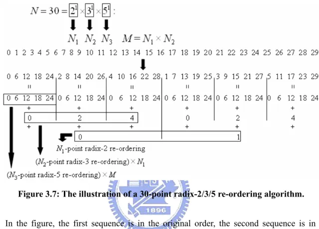
(35) (mA-1) times, ‘mB-stage’ means the data sequences are decimated by the radix-B algorithm (mB-1) times, ‘mC-stage’ means the data sequences are decimated by the radix-C algorithm (mC-1) times, ‘AmA×BmB-block and CmC-point’ means there are (AmA×BmB) data sequences with CmC sampling points for each sequence and ‘AmA-block and (BmB×CmC)-point’ means there are AmA data sequences with (BmB×CmC) data points for each sequence. For example, Figure 3.6 depicts the 30-point FFT computed by the radix-2/3/5 algorithm. We observe that the data sequence is decimated into two 15-point FFT’s first and then these two 15-point FFT’s are decimated into three 5-point FFT’s, respectively.. Figure 3.6: The 30-point FFT computed by the radix-2/3/5 algorithm.. This 30-point FFT can also be done by using other five algorithms of different order of 2, 3 and 5. Although the structures of computation and the order of input sequences are different, the obtained results are still the same.. 3.2.2. Re-Ordering Algorithm for Input Sequence. 23.

(36) Similar to section 3.1.2, here again we will find a mathematical relationship to describe the input order directly. We use radix-2/3/5 as an example to re-order a 30-point sequence in Figure 3.7. The procedure can be extended to the general case of the radix-A/B/C.. Figure 3.7: The illustration of a 30-point radix-2/3/5 re-ordering algorithm.. In the figure, the first sequence is in the original order, the second sequence is in the decimated order and the part written under the equal sign is the re-ordering algorithm. ‘N1-point radix-2 re-ordering’ means using bit-reversal (radix-2 re-ordering) to re-order the sequence of numbers 0…N1-1 where N1 is of the power of 2, and ‘(N2-point radix-3 re-ordering) × N1’ and ‘(N3-point radix-5 re-ordering) × M’ are similar to those discussed in section 3.1.2.. Chapter 4. Radix-2/4/3/5 FFT and Interpolation 24.

(37) Now we can use the radix-2/3/5 FFT to replace the radix-2 FFT, but we still want to speed up the radix-2/3/5 FFT and extend the numbers of sampling points to more numbers. To do this, we will replace the radix-2 algorithm in the radix-2/3/5 FFT with the radix-2/4 algorithm, thus we will obtain the radix-2/4/3/5 FFT. Furthermore, we will add the concept of interpolation to extend the applicable numbers of sampling points to any number.. 4.1. Radix-2/4/3/5 FFT Algorithm. For a data sequence x(n) with N (= 2m2’×3m3×5m5) sampling points, we replace the radix-2 algorithm with the radix-2/4 algorithm, in other words, we consider the data sequence x(n) to be N (= 2m2×4m4×3m3×5m5) sampling points. This reduces the number of computation stages since m2’ is larger than (m2 + m4). The computation of the radix-2/4/3/5 FFT is shown in Figure 4.1.. Figure 4.1: The radix-2/4/3/5 FFT decimation.. As for the re-ordering algorithm, it is the same as that of Figure 3.8, except that the N1-point radix-2 re-ordering must be replaced with the N1-point radix-2/4 re-ordering as shown in Figure 4.2.. 25.

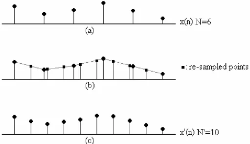
(38) Figure 4.2: The 30-point radix-2/4/3/5 re-ordering algorithm.. In the figure, the ‘radix-2/4 re-ordering’ is the radix-A/B re-ordering algorithm discussed in section 3.1.2.. 4.2. Interpolation Algorithm. The purpose of this algorithm is that it is to re-sample the sampled data so that the number of sampling points can be applied by the radix-2/4/3/5 FFT. For example, if there is a data sequence x(n) for a signal with N (= any number) sampling points, interpolation can re-sample x(n) and then we can obtain another similar sequence x’(n), which expresses the same signal, with N’ (= 2m2×4m4×3m3×5m5) sampling points. In order to shorten the run-time of interpolation and reduce the difference between x(n) and x’(n), we use the linear interpolation which is shown in Figure 4.3. In the figure, there is a data sequence x(n) with 6 sampling points in (a). We use a straight line passing through two points of x(n) to approximate the actual curve and then represent the interpolated signal with a new set of sequence x’(n) with 10 sampling points placed in equal time interval as shown in (c).. 26.

(39) Figure 4.3: The illustration of linear interpolation.. The following Figure 4.4 depicts the flow chart of an N-point FFT operated by the new algorithm.. N-point sampled data. find a number N’ m2 m4 m3 m5 to approximate N N’ = 2 ×4 ×3 ×5. N is any number interpolate the N-point sampled data to obtain another N’-point data. transform the N’-point data from time domain into frequency domain. radix-2/4,3,5 FFT algorithm. linear interpolation algorithm N’-point spectrum Figure 4.4: The flow chart of N-point FFT operated by the new algorithm.. 4.3. Simulation Results. To illustrate the advantage of the radix-2/4/3/5 FFT on the applicable number of sampling points, we do the following experiment: Within the range from 1 to 10000, we choose 50 groups of Ns evenly. The numbers of sampling points (Ns) and the data sequences are 27.

(40) obtained from the procedure as follows:. for (i=1:50) Ns(i)=111+(i-1)*200; for (j=1:Ns(i)) x(i,j)=j; end end We plot the required numbers of sampling points for which the FFT algorithms can be applied in terms of the number of sampling points for the single-radix FFT’s in Figure 4.5 and for the mixed-radix FFT’s in Figure 4.6.. Figure 4.5: The comparison of applicable number (Ni) of sampling points which can be applied by the single-radix FFT’s.. In the figure, ‘DFT’ means using discrete Fourier transform which can be applied with any number of sampling points. Thus ‘DFT’ is a straight line. The radix-2 FFT has the most numbers of sampling points than any other single-radix FFT as discussed in section 2.5 since it has the minimum step-level in the figure. The larger the decimating factor is, the larger the. 28.

(41) step-level is. Hence, it is not a good idea to use the single-radix FFT’s.. Figure 4.6: The comparison of applicable number (Ni) of sampling points which can be applied by the mixed-radix FFT’s.. Figure 4.6 shows the similar plots for the mixed-radix FFT’s. In the figure, ‘radix-2,3 FFT’ includes two algorithms, i.e., radix-2/3 FFT and radix-3/2 FFT, since they have the same number of re-sampled points. And so does for the ‘radix-2,5 FFT’ and ‘radix-2,3,5 FFT’. From the figure, we can find that ‘radix-2,3 FFT’, ‘radix-2,5 FFT’ and ‘radix-2,3,5 FFT’ all follow the straight line of ‘DFT’, and as Ns is larger, the step-levels of ‘radix-2,3 FFT’ and ‘radix-2,5 FFT’ are larger too. As for the ‘radix-2,3,5 FFT’, it has the smallest step-level and approaches that of the ‘DFT’.. 29.

(42) Figure 4.7: The comparison of ΔN (Ni - Ns) for different mixed-radix FFT’s.. Figure 4.7 shows the ΔN (Ni - Ns) plots which are derived from data from Figure 4.6 for each mixed-radix FFT. Obviously, ‘radix-2,5 FFT’ has the maximum amplitude and ‘radix-2,3,5 FFT’ has the minimum amplitude. To further demonstrate the above property is to plot the data in the form of 1 - |ΔN/Ns| versus the number of sampling points as shown in Figure 4.8.. Figure 4.8: The comparison of 1 - |ΔN/Ns| for different mixed-radix FFT’s. 30.

(43) Since interpolation modifies the original signal and introduces effectively noise to the signal, it is interesting to investigate how the S/N of the signal will be affected by the interpolation process. The 1 - |ΔN/Ns| figure reflects indirectly the S/N of the processed signal. In the figure, it can be seen that the radix-2,3,5 FFT has the best S/N than other two algorithms. However, as for other two algorithms, their S/N’s are not too bad since their values of 1 - |ΔN/Ns| are all larger than 0.9. Next, we will compare the run-time for different FFT algorithms. First we compare the run-times of the radix-2 FFT and the radix-2/4 FFT as shown in Figure 4.9 and then compare the run-times of the radix-2,3,5 FFT and the radix-2/4,3,5 FFT as shown in Figure 4.10 since they have the same numbers of re-sampled points, respectively.. Figure 4.9: The comparison of run-times of radix-2 FFT and radix-2/4 FFT.. Obviously, the radix-2/4 FFT is faster than radix-2 FFT and the run-time of radix-2/4 FFT is almost half of that of radix-2 FFT. This result is consistent with that of Table 2.3. In this experiment, for the radix-2/4 FFT, only the first stage is decimated by the factor 2, and all other stages are decimated by the factor 4. So, the radix-2/4 FFT is almost the same as the. 31.

(44) radix-4 FFT, except that the number of sampling points that can be applied to radix-2/4 FFT is of the power of 2, not of the power of 4.. Figure 4.10: The comparison of run-times of radix-2,3,5 FFT and radix-2/4,3,5 FFT.. In this experiment, the radix-2/4,3,5 FFT was obtained by replacing the radix-2 algorithm of the radix-2,3,5 FFT with the radix-2/4 algorithm. From this figure, we can see that the radix-2/4,3,5 FFT is faster than the radix-2,3,5 FFT, but there are some positions that these two algorithms overlap. This is because the numbers of re-sampled points are (2×3m3×5m5) where the radix-2/4,3,5 FFT is the same as the radix-2,3,5 FFT. The comparison of run-times of radix-2,3 FFT, radix-2,5 FFT and radix-2,3,5 FFT that have similar numbers of re-sampled points is shown in Figure 4.11 . Obviously, radix-2,3 FFT and radix-2,5 FFT have similar performance of computation speed but the radix-2,3,5 FFT has a better computation speed performance than the above two algorithms generally.. 32.

(45) Figure 4.11: The comparison of run-times of radix-2,3 FFT, radix-2,5 FFT and radix-2,3,5 FFT.. And the comparison of run-times of radix-2,3 FFT, radix-2,5 FFT and radix-2/4,3,5 FFT is shown in Figure 4.12. Obviously, radix-2/4,3,5 FFT is much better than other two algorithms.. Figure 4.12: The comparison of run-times of radix-2,3 FFT, radix-2,5 FFT and radix-2/4,3,5 FFT.. 33.

(46) As a conclusion, based on results of Figures 4.6, 4.7, 4.8 and 4.12, we can conclude that the radix-2/4,3,5 FFT cooperating with interpolation is the best algorithm in doing FFT which satisfy both the requirements of the performance of computation speed and the applicable numbers of sampling points.. 4.4. Examples. In this section we further use two examples applied with the above developed FFT algorithms to show their effectiveness. One example is to transform a multi-tone signal which is often used as a test input for a mixed signal testing, and the other is a square wave signal applied with the algorithm. The results are also shown in terms of the applicable number of sampling points, the run-time, and the introduced noise due to the interpolating the data points on the signal.. 4.4.1 Multi-tone Signal. Figure 4.13: The waveform of the multi-tone signal.. This signal contains 4 tones, the frequency and magnitude of each tone and the sampling. 34.

(47) frequency are shown as follows and the signal is plotted in Figure 4.13. The frequencies are described in the form of bin number.. f=[1 3 5 7]*115; m=[1 1 1 1]; nyquist=max(f)*2; for (i=1:50) fs(i)=nyquist+1+(i-1)*200; end We plot the required numbers of sampling points for which the FFT algorithms can be applied in terms of the number of sampling points for the FFT’s in Figure 4.14. Still, we can see that the radix-2/4,3,5 algorithm is the best algorithm which can take the most of number of applicable data points while other algorithms all have limited number of applicable data points.. Figure 4.14: The comparison of applicable number (Ni) of sampling points which can be applied by the FFT’s.. Next, we will compare the run-time for different FFT algorithms as shown in Figure 4.15.. 35.

(48) Figure 4.15: The comparison of run-times of different FFT algorithms.. In the figure, we can see that the radix-2/4,3,5 algorithm has the best run-time among all the algorithms except the radix-2/4 algorithm. The radix-2/4 algorithm has the least run-time because the number of data points are less than that of the radix-2/4,3,5 algorithm.. Figure 4.16: The comparisons of magnitudes of each tone of different FFT algorithms (a) 1st tone, (b) 2nd tone, (c) 3rd tone, and (d) 4th tone.. 36.

(49) Figure 4.16 plots the obtained magnitudes of each tone in terms of the number of data points for each algorithm. For reference, the magnitudes obtained by using the DFT, which can be considered to be the ideal case transformation, are also plotted. It is seen that the magnitudes of the tones obtained through all FFT algorithms increase with the number of data points since more data points more accurate the obtained values. Figure 4.17 shows the combined magnitude of the four tones where we see the same trend.. Figure 4.17: The comparison of magnitudes of signal of different FFT algorithms.. Figure 4.18 plots the introduced noises in terms of the number of data points due to interpolating process for each algorithm. Figure 4.18 (a) also includes the noise obtained for the original four-tone signal if the DFT algorithm is used as the transforming algorithm. It is seen that for all FFT algorithms, much noises are introduced on the transformed spectrums due to the interpolating process which makes the interpolated signal different from the original signal. Figure 4.18 (b) shows the expanded plot of the Figure 4.18 (a)’s plot to show the noise introduced for each FFT algorithm. It is seen that for all algorithms, except the radix-2/4,3,5 one, the noises oscillate with the number of data points since the number of. 37.

(50) interpolating data points increase periodically with respect to the number of interpolated data points. The introduced noise for the radix-2/4,3,5 algorithm decreases monotonically with respect to the number of interpolated data points.. Figure 4.18: The comparisons of magnitudes of noise of different FFT algorithms (a) with DFT value as a reference, and (b) without DFT value.. If we express the above in terms of S/N of the signal with respect to the noise induced by the interpolation process, the difference between different algorithms can be more clearly seen. Figure 4.19 plots the S/N of each tone and Figure 4.20 plots the S/N for the combined waveform of tones. It is seen that the radix 2/4,3,5 algorithm has the largest S/N.. 38.

(51) Figure 4.19: The comparisons of S/N’s of each tone of different FFT algorithms (a) 1st tone, (b) 2nd tone, (c) 3rd tone, and (d) 4th tone.. Figure 4.20: The comparison of S/N’s of signal of different FFT algorithms.. 4.4.2 Square Wave A square wave signal is a signal composed of infinite number of frequencies and is a good signal for making the experiment of applying the developed algorithms. Here we use ten tones. 39.

(52) to approximate the square wave. Figure 4.21 shows the magnitude of each tone, the DC value, and the sampling frequency for the signal analyzed.. Figure 4.21: The waveform of the square wave.. f=[1 3 5 7 9 11 13 15 17 19]*42; m=[0.637 0.212 0.127 0.091 0.071 0.058 0.049 0.043 0.038 0.034]; DC=0.5; nyquist=max(f)*2; for (i=1:50) fs(i)=nyquist+1+(i-1)*200; end Figures 4.22, 23, 24, 25, and 26 are the corresponding respective figures of this example as the Figures 4.14, 15, 17, 18, and 20 of the previous example. We can see the similar phenomena as those observed in the Figures 4.14, 15, 17, 18, and 20. The only difference is that since for the square wave, its waveform is mainly determined by the first several fundamental and harmonics frequency components, the sampling frequency selected for this wave is the Nyquist frequency of the last tone of this square wave. This makes the sampling. 40.

(53) frequency far above than the fundamental tone of this wave and the sampling points are much more than the case of the previous example. This consequently makes the noise introduced due to interpolation less.. Figure 4.22: The comparison of applicable number (Ni) of sampling points which can be applied by the FFT’s.. Figure 4.23: The comparison of run-times of different FFT algorithms.. 41.

(54) Figure 4.24: The comparison of magnitudes of signal of different FFT algorithms.. Figure 4.25: The comparisons of magnitudes of noise of different FFT algorithms (a) with DFT value as a reference, and (b) without DFT value.. 42.

(55) Figure 4.26: The comparison of S/N’s of signal of different FFT algorithms.. In summary, from the experiment results on these two examples, the radix-2/4,3,5 FFT exhibits the best performance on the run-time and the S/N over the radix-2,3 FFT and the radix-2,5 FFT algorithms. For the radix-2/4 algorithm, it has a good performance on the run time due to its less number of sampling points, however, it produces too much noise when interpolation is used.. 43.

(56) Chapter 5. Conclusion. In this thesis, we have proposed and studied the mixed-radix FFT algorithm to speed up the conventional radix-2 FFT algorithm. In the work, we first studied the single-radix FFT and derived the decimation-in-time algorithm, the process of re-ordering the data sequence, and discussed the applicable numbers of sampling points which can be applied by the FFT algorithm. Then based on this, we further studied the mixed-radix FFT algorithm. We first derived the algorithm with two radixes, i.e., radix-A/B FFT, by directly applying the decimation-in-time algorithm and deriving a mathematical relationship for the decimated order. And then, we derived the radix-A/B/C FFT which is much faster than the conventional radix-2 FFT algorithm. An additional advantage of the algorithm is that the numbers of sampling points which can be applied by the FFT algorithm have been increased a lot. To further extend the use of the mixed-radix FFT, we adopt the interpolation technique to re-sample the original signal to make the number of sampling points to be applicable by the mixed-radix algorithm. We studied interpolation for the radix-2,3 FFT, the radix-2/4 FFT, the radix-2,5 FFT and the radix-2,3,5 FFT and found that the radix-2,3,5 FFT cooperates with interpolation has the best performance. Furthermore, we extended it to the radix-2/4,3,5 FFT to further improve the computation speed of the algorithm.. 44.

(57) References [1]. Mark Burns and Gordon W. Roberts, “An Introduction to Mixed-Signal IC Test and Measurement,” New York Oxford University Press, 2001, ISBN: 0195140168.. [2]. J. W. Cooley and J. W. Tukey, “An Algorithm for Machine Computation of Complex Fourier Series,” Math. Comput., vol. 9, pp. 297-301, 1965.. [3]. Duhamel P. and Vetterli M., “Fast Fourier Transforms: A Tutorial Review,” Signal Processing 19, pp. 259-299, 1990.. [4]. Robert W. Ramirez, “The FFT Fundamentals and Concepts,” Prentice Hall, Englewood Cliffs, NJ 07632, January 1985, ISBN: 0133143864.. [5]. Paul Bourke, “DFT (Discrete Fourier Transform) FFT (Fast Fourier Transform),” June 1993, http://astronomy.swin.edu.au/~pbourke/analysis/dft/.. [6]. “Fast Fourier Transform (FFT),” http://www.cmlab.csie.ntu.edu.tw/cml/dsp/traning/coding/transform/fft.html.. [7]. “Fast Fourier Transform Tutorial,” http://astron.berkely.edu/~jrg/ngst/fft/fft.html.. [8]. Y. Suzuki, T. Sone, and K. Kido, “A New Algorithm of Radix 3, 6, and 12,” IEEE Trans. Acoust., Speech, Signal Processing, vol. ASSP-34, pp. 380-383, Feb. 1986.. [9]. Soo-Chang Pei and Wei-Yu Chen, “Split Vector-Radix-2/8 2-D Fast Fourier Transform,” IEEE Signal Processing Lett., vol.11, pp. 459-462, May 2004.. [10]. S. Bouguezel, M. O. Ahmad, and M. N. S. Swamy, “An Efficient Split-Radix FFT Algorithm,” in Proc. IEEE Int. Symp. on Circuits and Systems Bangkok, Thailand, vol. 4, pp. 65-68, May 2003.. [11] M. Vetterli and P. Duhamel, “Split-Radix Algorithms for Length-pm DFT’s,” IEEE. 45.

(58) Trans. Acoust., Speech, Signal Processing, vol. ASSP-37, pp. 57-64, Jan. 1989. [12]. G. Bi and Y. Q. Chen, “Fast DFT Algorithms for Length N = q*2m,” IEEE Trans. Circuits Syst. II, vol. 45, pp. 685-690, June 1998.. [13]. Bouguezel S., Ahmad M.O., and Swamy M.N.S, “A New Radix-2/8 FFT Algorithm for Length-q×2m DFTs,” IEEE Trans. Circuits Syst. I, vol. 51, pp. 1723-1732, Sept. 2004.. 46.

(59) 簡姓. 名：陳見明. 性. 別：男. 生. 日：民國七十年十月二十四日. 籍. 貫：臺灣省新竹縣. 歷. 通訊地址：台中市西屯區寧夏東三街 17-1 號 7F 之 8. 學. 歷：民國九十二年二月至民國九十四年六月. 國立交通大學電子研究所碩士班. 民國八十八年九月至民國九十二年一月. 國立中正大學電機工程學系. 論文題目：應用於混模電路測試之利用混合基底與內插法的快速傅立葉轉換 FFT Based on Mixed-Radix and Interpolation for Mixed-Signal Testing. 47.

(60)