應用於H.264/AVC 1080HD的高產量背景適應性二元算術編解碼器

國

立

交

通

大

學

電機學院 IC 設計產業研發碩士班

碩

士

論

文

應用於 H.264/AVC 1080HD 的高產量背景適應性二

元算術編解碼器

A High Throughput Context Adaptive Binary

Arithmetic Codec for H.264/AVC 1080HD

Application

研 究 生：林秉昌

應用於 H.264/AVC 1080HD 的高產量背景適應性二元算術編解

碼器

A High Throughput Context Adaptive Binary Arithmetic Codec

for H.264/AVC 1080HD Application

研 究 生：林秉昌 Student：Ping-Chang Lin

指導教授：李鎮宜 教授 Advisor：Dr. Chen-Yi Lee

國 立 交 通 大 學

電機學院

IC 設計產業研發碩士班

碩 士 論 文

A Thesis

Submitted to College of Electrical and Computer Engineering National Chiao Tung University

in partial Fulfillment of the Requirements for the Degree of

Master in

Industrial Technology R & D Master Program on IC Design

January 2007

Hsinchu, Taiwan, Republic of China

應用於 H.264/AVC 1080HD 的高產量背景適應性二元算

術編解碼器

學生：林秉昌 指導教授：李鎮宜 教授

國立交通大學

電機學院產業研發碩士班

摘要

在本論文中，我們對算數編碼器提出三個提升生產率的方法以提高整個背景 適應性二元算數(CABAC)編碼器的產率，此外我們也對 CABAC 編解碼器提出硬 體共享的方法以降低其硬體成本。關於我們的解碼器部份，我們沿用我們在2006 年 8 月份所發表的高產率 CABAC 解碼器 [2]。我們所提出的提高產率的方法主 要是以所統計的資料分布特性來設計，這可以改善資料相依特性所產生的產率受 限制情形。我們所提出的架構可以達到平均每秒處裡245760 個巨方塊，在編碼時 可以滿足層次4.1，而在解碼時可以滿足層次 4.0。因此，這足以對 1080HD 格式 每秒三十張畫面的影像做即時編解碼。基於0.18 微米聯華電子互補式金氧半導體 製程，我們的CABAC 編解碼器設計需要 173303 個邏輯閘(含 SRAM)，其操作時

A High Throughput Context Adaptive Binary

Arithmetic Codec for H.264/AVC 1080HD Application

Student：Ping-Chang Lin Advisor：Prof. Chen-Yi Lee

Industrial Technology R & D Master Program of

Electrical and Computer Engineering College

National Chiao Tung University

ABSTRACT

In this thesis, we propose three high throughput methods for arithmetic encoder to promote the throughput of CABAC encoder and some hardware sharing methods for CABAC codec to lower its cost. About the decoder of our CABAC codec, we continue using the high throughput CABAC decoder [2] which we presented in August 2006. The proposed high throughput methods are based on the results of data statistic, they can improve the restriction in throughput caused by data dependence. Our proposed architecture can achieve 245760 macroblocks per second in average for level 4.1 in encoding and for level 4.0 in decoding. Therefore, it is sufficient to support 1080HD for real-time encoding/decoding at 30fps. Based on 0.18 μm UMC CMOS Process, our

誌 謝

首先要感謝恩師 李鎮宜教授，在老師的細心指導下，不但習得做研究的方 法，且逐漸建立了老師一直強調的系統層級設計考量的設計觀念。這使我在微觀 的設計同時，也漸漸可以用巨觀的角度審視自己的設計是否滿足系統的需求。在 每次會議報告中老師給予的寶貴意見及 SI2 實驗室提供了優良的積體電路設計環 境，使我在研究上能更順利的完成。 再來是感謝SI2 實驗室的學長 : 毅宏、康正、俊彥、陳元，及同學們 : 皆賢、 岳琪、大嘉、堉棋、名威、文平、義閔的指導幫助，其中黃毅宏 學長更是細心指 導我在硬體設計上正確觀念的建立。在交大研究所這兩年，大家一起熬過艱難日 子所培養出的革命情感，使我衷心希望大家都有著美好的未來。 最後要感謝我的 父母的關心與協助，使我能無後顧之憂得專心在做研究上。 謹將此論文獻給關心及愛護我的家人與朋友們。

Contents

Chapter 1 Introduction... 1

1.1 Motivation... 1

1.2 Organization of thesis ... 2

Chapter 2 Algorithm of CABAC for H.264/AVC... 4

2.1 Overview of CABAC encoding/decoding flow... 5

2.2 Binarization process... 8

2.2.1 Unary (U) binarization process... 8

2.2.2 Truncated unary (TU) binarization process ... 10

2.2.3 Fixed-length (FL) binarization process ... 12

2.2.4 Unary/k-th order Exp_Golomb (UEGk) binarization process ... 13

2.2.5 Special binarization process ... 15

2.3 1Algorithm Of basic binary arithmetic coding ... 19

2.3.1 Basic binary arithmetic encoding algorithm ... 20

2.3.2 Basic binary arithmetic decoding algorithm ... 22

2.4 Advanced binary arithmetic coding for H.264/AVC... 24

2.5 Context model organization ... 35

2.6 Syntax elements for the neighbor blocks... 40

2.7 Paper survey for state-of –the-art CABAC designs ... 43

Chapter 3 Binary Arithmetic Encoding Engine ... 47

3.1 Overview of CABAC... 48

3.2 Three throughput promoting methods... 51

3.2.1 Multi-symbol architecture... 52

3.2.2 Pipeline organization ... 60

3.2.3 Case Efficiency Architecture ... 63

3.2.3.1 Throughput bottleneck of arithmetic encoding engine 64 3.2.3.2 Throughput efficiency design... 66

3.2.3.3 Cost issue in output interface ... 79

3.2.3.4 Cost efficiency design... 80

Chapter 4 CABAC Codec System Architecture ... 85

4.1 Hardware sharing methods ... 85

4.2 Memory requirement... 89

Chapter 5 Simulation and Implementation Result for Digital TV Application... 91

5.1 Specification of different levels ... 92

6.1 Conclusion... 100 6.2 Future work ... 101 6.3 Discussion from H.264/AVC system view... 101

3

Bibliography ... 104

4

List of Figures

Figure 1 H.264/AVC encoder/decoder system block diagram... 5

Figure 2 CABAC encoder flow chart [4]... 6

Figure 3 CABAC decoder flow chart ... 7

Figure 4 (a) Definition of MPS and LPS ... 20

Figure 4 (b) Sub-divided interval of MPS... 20

Figure 4 (c) Sub-divided interval of LPS ... 20

Figure 5 (a) Result of MPS subdivision... 23

Figure 5 (b) Result of LPS subdivision... 23

Figure 6 Flowchart of the normal encoding flow [1] ... 25

Figure 7 Flowchart of renormalization in the encoder [1] ... 26

Figure 8 Flowchart of PutBit(B) [1] ... 27

Figure 9 Flowchart of encoding bypass [1] ... 28

Figure 10 Flowchart of the terminal encoding flow [1] ... 29

Figure 11 Flowchart of flushing at termination[1]... 30

Figure 12 Flowchart of the normal decoding flow [1] ... 32

Figure 13 Flowchart of renormalization in the decoder [1] ... 33

Figure 14 Flowchart of the bypass decoding flow [1] ... 34

Figure 16 Illustration of the neighbor location in macroblock level ... 41

Figure 17 Illustration of the neighbor location for sub-macroblock level ... 42

Figure 18 Arithmetic coding interval update. (a) Complete iteration. [11] ... 44

Figure 18 Arithmetic coding interval update. (b) range updating. [11] ... 44

Figure 18 Arithmetic coding interval update. (c) Pre-computations for low updating. [11] ... 44

Figure 19 CABAC & MZ pseudo-code description [9]... 45

Figure 20 Sample update of codlLow [12] ... 46

Figure 21 System architecture of CABAC encoder ... 48

Figure 22 System architecture of CABAC decoder ... 50

Figure 23 Percentage of the usage of the three encoding modes in AE ... 51

Figure 24 Percentage of the number of the concatenate bypass encoding per bypass demand under executing CIF frames for four typical video sequences... 54

Figure 25 Percentage of the number of the concatenate bypass encoding per bypass demand under executing 1080HD frames for two typical video sequences... 55

Figure 26 Bypass encoding unit ... 57

Figure 27 Architecture of the multi-symbol bypass encoding... 58

Figure 28 Timing diagram of the pipeline comparison ... 60

Figure 31 Statistic of bitsOutstanding for the low complexity and slow motion

video sequence ... 66

Figure 32 Statistic of bitsOutstanding for the high complexity and fast motion video sequence ... 67

Figure 33 Statistic of bitsOutstanding for 1080HD video sequence ... 68

Figure 34 Tree map of the renormalization process... 69

Figure 35 Illustration of the shifting left of codlLow ... 74

Figure 36 Probabilities of the different containing range of remainder bitsOutstaning based on Table 17 ... 76

Figure 37 Case Efficiency Architecture for renormalization process... 77

Figure 38 The proposed bit-stream output interface ... 81

Figure 39 Three main parts of CABAC encoder... 87

Figure 40 Illustration of hardware sharing for CABAC encoder and decoder.. 87

Figure 41 Architecture of the hardware sharing CABAC codec system... 88

Figure 42 The required memory size of our CABAC codec system ... 89

Figure 43 The characteristic curves of station video sequence (QP: 42 ~ 16) .... 94

Figure 44 The characteristic curves of riverbed video sequence (QP: 42 ~ 16) . 95 Figure 45 System block diagram of H.264/AVC decoding for main profile ... 102

List of Tables

Table 1 bin string of the unary binarization [1]... 9

Table 2 bin string of the fixed-length code ... 12

Table 3 Binarization for macroblock types in I slice... 16

Table 4 Binarization for macroblock types in P, SP, and B slices ... 18

Table 5 Binarization for sub-macroblock types in P, SP, and B slices... 19

Table 6 Value of ctxIdxOffset definition [1] ... 37

Table 7 Assignment of ctxBlockCat due to coefficient type [1]... 37

Table 8 Assignment of ctxIdxBlockCatOffset due to ctxBlockCat and syntax elements of the residual data [1] ... 38

Table 9 Definition of the ctxIdxInc value for context model index [1]... 38

Table 10 Required syntax elements of the left and top neighbor blocks and the computation for ctxIdxInc... 39

Table 11 Assignment of ctxIdx for syntax element mbType... 39

Table 12 The cases corresponding to its accumulating number of bitsOutstanding=7 (It is under last remainder bitsOutstanding=0) ( 4 cases ) ... 70

Table 13 The cases corresponding to its accumulating number of bitsOutstanding=6 (It is under last remainder bitsOutstanding=0) ( 12 cases ) ... 71

Table 14 The cases corresponding to its accumulating number of

bitsOutstanding=5 (It is under last remainder bitsOutstanding=1)

( 32 cases ) ... 71

Table 15 The number of the corresponding cases for the accumulating number of bitsOutstanding of one symbol... 73

Table 16 The utility rate of each case for one symbol ... 75

Table 17 The number of cases and the probabilities of the different containing range of remainder bitsOutstanding ... 76

Table 18 The relationship between shift and codlRange ... 79

Table 19 Probability of bitsOutstanding being greater than 7... 80

Table 20 Required buffer slot for the different length bit-stream ... 82

Table 21 The states of FSM which are similar procedures between binarization and debinarization ... 86

Table 22 Maximum frame rates (fps) for some different frame types [1]... 92

Table 23 level limits [1] ... 93

Table 24 The proposed arithmetic encoder comparing with the existing designs ... 96

Table 25 The proposed CABAC codec comparing with the existing CABAC designs ... 96

Table 26 Percentage of the cycle reduction for the proposed three throughput promoting methods ... 98

Chapter 1

Introduction

1.1 Motivation

H.264/AVC is the state-of-the-art video coding standard developed by ITU-T Video Coding Experts Group and ISO/IEC Moving Picture Experts Group (MPEG). The new standard provides gains in compression efficiency of up to 50% over a wide range of bit rates and video resolutions compared with the former standards such as H.263 and MPEG-4 by employing many innovative technologies such as multiple reference frame, variable block size motion estimation, in-loop de-blocking filter and context-based adaptive binary arithmetic coding (CABAC). Because of its outstanding performance in quality and compression gain, the H.264/AVC is adopted to be video standard in more and more consumer application products such as digital video recorder / player, portable video device…etc.

H.264/AVC contains two alternative entropy coding schemes which are context-based adaptive variable length coding (CAVLC) and context-based adaptive binary arithmetic coding (CABAC). The simpler entropy coding method is CAVLC for simple profile. It can save about 10% for the execution time under increasing about 7% bit-rate compared with CABAC. Because of bit-rate saving, CABAC is the superior scheme for massive capacity demand of the newest video application.

inevitable complexity overhead. The results of the software-based complexity analysis are presented in [3], which claims that switching from CAVLC to CABAC usually leads to complexity increasing by 25% ~ 30% for encoding and 12% for decoding, in terms of access frequency (total number of memory transfers per second); therefore, both the coding acceleration and the cost efficiency promoting of CABAC are required.

We propose three throughput promoting methods to make CABAC encoder achieve the specification of 1080HD in level 4.1 stipulated in H.264/AVC standard [1]. For CABAC decoder, we continue using the high throughput CABAC decoder [2] which we presented in August 2006. It can achieve the specification of 1080HD in level 4.0. So our CABAC codec is sufficient to support 1080 HD video for real-time encoding and decoding at 30 fps. Besides, we also introduces some low cost methods such as finite state machine sharing, table reuse…etc to make the CABAC codec be better cost efficiency.

1.2 Organization of this thesis

This thesis is organized as follows. In Chapter 2, we present the algorithm of CABAC. It contains two levels coding procedure. For encoding, the first level is binarization engine, and the second level is arithmetic encoder. For decoding, the order of the two levels procedure is just opposite to encoding. Chapter 3 focuses on throughput promoting. We introduce three arithmetic encoding modes, and showing the proposed three high throughput methods. Chapter 4 focuses on cost efficiency designing. We present the proposed low cost methods and the memory requirement. In the end of this chapter, we show the proposed CABAC codec system architecture

simulation and chip implementation will be shown in Chapter 5. We make a brief conclusion and future work in the last chapter.

Chapter 2

Algorithm of CABAC for

H.264/AVC

In this chapter, we introduce the algorithm of CABAC encoding and decoding respectively. Both CABAC encoding and CABAC decoding are composed of three parts: the binarization process, the arithmetic coding process and the context model. For CABAC encoding, the binarization process reads syntax elements (SE), then computing the bin to offer the arithmetic encoding process for encoding the corresponding bit-streams. For CABAC decoding, the arithmetic decoding process reads the input bit-streams generated by H.264 encoder, and computing the bin to offer the binarization process for decoding the suitable SE. Both arithmetic encoding and arithmetic decoding have to look up context model which records the historical probability to compute the corresponding bit-streams in encoding and the bin value in decoding.

About the description of CABAC algorithm in this chapter, it is based on the content of [1] and [5], where the latter only focuses on decoding aspect, and the encoding aspect is introduced in addition in this chapter.

This chapter is organized as follows. In Section 2.1, we present the overviews of the CABAC encoding and decoding flow respectively, and show the two levels coding processe. In Section 2.2, we introduce all kinds of the binarization process such as the

organization. In Section 2.3, the algorithm of basic binary arithmetic coding will be introduced briefly. We introduce it in terms of encoding and decoding respectively in the section 2.3.1 and the section 2.3.2. In Section 2.4, we present the advanced binary arithmetic coding for H.264/AVC, and relating it to arithmetic coding process. Section 2.5 shows the context model related to the different SEs. In final section, what we show is that how to get the neighbor SE to index the suitable context model allocation.

2.1 Overview of CABAC encoding/decoding flow

Intra Frame Prediction Frame Storage Motion Compensation Motion Estimation De-blocking Filter + -+ Quantization DCT Inverse Quantization IDCT Entropy Encoding H.264 Bitstream Video Input ( Y U V ) H.264 Encoder Inverse Quantization IDCT Entropy Decoding H.264 Bitstream De-blocking Filter Intra / Inter Intra / Inter Motion Compensation Intra Frame Prediction Frame Storage Video Output ( Y U V ) H.264 Decoder +

Figure 1 H.264/AVC encoder/decoder system block diagram

Figure 1 shows the system block diagram of H.264/AVC encoder and decoder. Both entropy encoder and entropy decoder contain three entropy coding strategies such as universal variable length coding (UVLC), context-based adaptive variable length coding (CAVLC) and context adaptive binary arithmetic coding (CABAC).

For H.264/AVC baseline profile, it only adopts UVLC and CAVLC two variable length coding (VLC) strategies to code the macroblock (MB) information and the pixels coefficients. UVLC is one of VLC in baseline profile, it codes not only the MB information such as the mb_type, coded_block_pattern, intra_prediction_mode, and so on, but also the MB coefficient such as mvd. Because the residual data coding occupies over 50% of the entire execution time, the residual coefficients are computed by the CAVLC architecture for more efficiency.

For H.264/AVC main profile, it has an advance choice except VLC. CABAC can be used in place of UVLC and CAVLC. Thus, H.264 system just needs CABAC to code all MB information and pixel data if entropy coding flag is assigned to CABAC.

In this section, we introduce the block diagram of CABAC encoder and decoder. Then, the execution flow of them will be introduced respectively meanwhile.

Binarization Context _Modeler Normal Coding Engine Bypass Coding Engine bin bin normal bypass bypass normal bin value for context model update

bit stream coded bits

coded bits Binary Arithmetic Coder loop over bins bin string binary valued syntax element non-binary valued syntax element syntax element bin, Context modeler

Figure 2 CABAC encoder flow chart [4]

Figure 2 shows the block diagram of CABAC encoder. We first see the left side of this figure. All syntax elements (SEs) of the H.264/AVC will be transferred into the binary code “bin” when entering the CABAC encoding process. Besides the SE of fixed-length coding type, all SEs have to be encoded by the binarization process which

by the binary arithmetic encoder. The binary arithmetic encoder has three different encoding types such as normal, bypass and terminal encoding processes. The terminal encoding process is seldom applied in CABAC system, which is only executed one time per macroblock (MB) encoding flow when the current MB is complete. So we ignore its influence due to its seldom applying opportunities. The normal and bypass encoding process are two main binary arithmetic coding modes. If it performs the bypass encoding process, there is no need to refer to the context model because the probability of bit-stream value is equal (probability = 0.5) between logical “1” and “0”. If it applies the normal encoding process, it has to refer the associated context model depending on the SE type and the bin index.

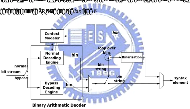
Binarization Normal Decoding Engine Bypass Decoding Engine bypass normal bit stream

Binary Arithmetic Deoder

loop over bins bin string syntax element Context Modeler bin bin bin string

Figure 3 CABAC decoder flow chart

Figure 3 shows the block diagram of CABAC decoder. In H.264/AVC decoder, the decoding flow is contrary to CABAC encoder. At first, the binary arithmetic decoder reads the bit-stream and transfers it to be bin string. The binarization process reads the bin string and decodes it to be SE by five kinds of decoding flows. The execution sequences between CABAC encoder and decoder are just reverse. But the

and CABAC decoder.

2.2 Binarization process

In Section 2.2, we focus on the binarization process. In CABAC encoder, it reads the syntax element and transfers it to be bin string. In CABAC decoder, it reads the bin string to look up the suitable syntax element. For H.264/AVC, both CABAC encoder and CABAC decoder adopt five kinds of the binarization methods to encode/decode the syntax element/bin string respectively. This section is organized as follows. In Section 2.2.1, the flow of the unary code is shown at first. The unary code is the basic coding method. Section 2.2.2 shows the truncated unary code which is the advanced unary coding method. In Section 2.2.3, we introduce the fixed-length coding flow. It is the typical binary integer method. Section 2.2.4 is the Exp-Golomb coding flow. The Exp-Golomb coding flow is only used for the residual data and the motion vector difference (mvd). Section 2.2.5 is the special definition which is by means of the table method. Specifically, we focus on the binary tree of the macroblock type (mb_type) and the sub-macroblock type (sub_mb_type).

2.2.1 Unary (U) binarization process

Input to this process is a request for a U binarization for a syntax element. Output of this process is the U binarization of the syntax element.

The bin string of a syntax element having value synElVal is a bit string of length synElVal + 1 indexed by binIdx. The bins for binIdx less than synElVal are equal to “1”. The bin with binIdx equal to synElVal is equal to “0”.

the syntax element is equal to “0”, the bin outputs single bit “0”. Except the syntax element “0”, the bin string sends numSE “1” and one “0” in the end of the binary value. The value of numSE is equal to the syntax element. Therefore, we find that the bin string length of current syntax element is numSE + 1.

Table 1 bin string of the unary binarization [1]

Syntax

element bin string

0 0 1 1 0 2 1 1 0 3 1 1 1 0 4 1 1 1 1 0 5 1 1 1 1 1 0 … …… binIdx 0 1 2 3 4 5

According to the unary bin string format shown above, we arrange the encoding and decoding algorithm in Eq. 1 and Eq. 2. These two equations represent the pseudo code of the unary encoding/decoding flow.

For unary encoding, it gets the binIdx which is the index of the bin string in Table 1 from the value of the input syntax element (SEVal). The for loop in Eq. 1 generates the bin string according to the binIdx. When finishing the for loop, it will generate one bit “0” as the end bit of the corresponding bin string. Namely, the unary binarization process arrives at the end of encoding step.

For unary decoding, it sets binIdx to zero at the initial step. The while loop in Eq. 2 checks the current bin assigned by binIdx from the bin string and binIdx counts if the

process arrives at the end of decoding step. binIdx sends to SEVal which is defined as the value of the syntax element.

Start unary (U) encoding process

binIdx = SEVal;

for (i == 0; i < binIdx; i ++ ){ bin = 1;

}

bin = 0; (Eq. 1)

Start unary (U) decoding process

binIdx = 0;

while (bin[binIdx] == 1){ binIdx = binIdx + 1; }

SEVal = binIdx; (Eq. 2)

2.2.2 Truncated unary (TU) binarization process

Input to this process is a request for a TU binarization for a syntax element and cMax. Output of this process is the TU binarization of the syntax element.

For syntax element values less than cMax, the U binarization process mentioned in Section 2.2.1 is invoked. For the syntax element value equal to cMax the bin string is a bit string of length cMax with all bins being equal to “1”. TU binarization is always invoked with a cMax value equal to the largest possible value of the syntax element.

The truncated unary binarization process is based on the unary one and has an additional factor of cMax which is defined as the maximum length of the current bin string. If the value of syntax element (SEVal) is less than cMax, the truncated unary

number “1” of the bin string is equal to cMax and there is no “0” bit in the end of the current string. For example, SEVal(=“4”) is assumed. If the value of cMax is “5”, the result of bin string is equal to “11110”. If the value of cMax is also “4”, the result of the bin string is equal to “1111” where the end bit of “0” is truncated in this case.

Eq. 3 is the truncated unary encoding flow which is modified from Eq. 1. Besides checking the value of syntax element (SEVal), it also takes cMax into consideration. If SEVal is less than cMax, it works as the unary encoding process. If binIdx isn’t less than cMax, it doesn’t generate “0” in the end of bin string when completing the encoding of current syntax element.

Start truncated unary (TU) encoding process

binIdx = SEVal;

for (i == 0; i < binIdx; i ++ ){ bin = 1;

}

If (SEVal < cMax) bin = 0; (Eq. 3)

Eq. 4 is the truncated unary decoding flow which is modified from Eq. 2. Besides checking the bin value, it takes cMax as a factor, additionally. It works as the unary decoding process when binsIdx is less than cMax. If binIdx isn’t less than cMax, it doesn’t complete the decoding action until reading the end bit “0” in the end of the bin string.

Start truncated unary (TU) decoding process

binIdx = 0;

while (bin[binIdx] == 1 && (binIdx < cMax)){ binIdx = binIdx + 1;

2.2.3 Fixed-length (FL) binarization process

Input to this process is a request for a FL binarization for a syntax element and cMax. Output of this process is the FL binarization of the syntax element.

FL binarization is constructed by using an fixedLength-bit unsigned integer bin string of the syntax element value. The indexing of bins for the FL binarization is such that the binIdx = 0 relates to the least significant bit with increasing values of binIdx towards the most significant bit.

The fixed-length code is the simple-defined format of the binarization coding process which is defined as the typical unsigned integer. The coding rule is represented by means of the typical binary number. For example, the value of “510” is equal to

“1012”. The value of “510” is defined as the decimal style and the value of “1012” is the

binary format which is the required fixed-length code. Table 2 shows the fixed-length code definition.

Table 2 bin string of the fixed-length code

Syntax

element bin string

0 0 0 0 0 0 0 1 0 0 0 0 0 1 2 0 0 0 0 1 0 3 0 0 0 0 1 1 4 0 0 0 1 0 0 5 0 0 0 1 0 1 … binIdx 0 1 2 3 4 5

For fixed-length encoding process, the value of input syntax element defines the binIdx. The value of (binIdx + 1) is just the required bit numbers for the corresponding bin string of the current syntax element.

because the maximum value of binIdx is five. All syntax elements which are decoded by the fixed-length format are always represented with six binary bits.

2.2.4 Unary/k-th order Exp_Golomb (UEGk)

binarization process

Input to this process is a request for a UEGk binarization for a syntax element, signedValFlag and uCoff. Output of this process is the UEGk binarization of the syntax element.

A UEGk bin string is a concatenation of a prefix bit string and a suffix bit string. The prefix of the binarization is specified by invoking the TU binarization process for the prefix part [ Min( uCoff, Abs( synElVal ) ) ] of a syntax element value synElVal as specified in Section 2.2.2 with cMax = uCoff, where uCoff > 0. Namely, the prefix part is dominated by cMax. The suffix part of this code doesn’t always apply because it isn’t adopted by two cases.

The UEGk bin string is derived as follows:

¾ If one of the following is true, the bin string of a syntax element having value synElVal consists only of a prefix bit string. Namely, the UEGk doesn’t enter the suffix coding step.

1. If signedValFlag is equal to 1 and the prefix bin contains only one 0 bit, the value of syntax element is just decided by prefix bin string with truncated unary (TU) code.

2. If signedValFlag is equal to 0 and the prefix bin string isn’t equal to the bit string which is composed of the string length cMax of bit 1.

¾ Otherwise, the bin string of the UEGk suffix part of a syntax element value synElVal is specified by a process equivalent to the following pseudo-code: If( Abs( synE1Val) >= uCoff){

sufS = Abs( synElVal) – uCoff stopLoop = 0 do{ if( sufS >= ( 1<<k)){ put( 1 ) sufS = sufS – ( 1<<k) k++ }else{ put( 0 ) while( k--)

put(( sufS >> k) & 0x01)

stopLoop = 1

}

} while( !stopLoop) }

If( signedValFlag && synElVal != 0) If( synElVal > 0)

put( 0 )

else

put( 1 ) (Eq. 5)

The initial value of k is defined as the order of the unary Exp-Golomb coding which are named as UEGk. In the binarization decoding of CABAC, it only applies two decoding flows such as UEG0 and UEG3. UEG0 is used by the residual data decoding process and UEG3 is used by the motion vector difference one.

2.2.5 Special binarization process

Input to this process is a request for a binarization for syntax element mb_type or sub_mb_type. Output of this process is the binarization of these two syntax elements.

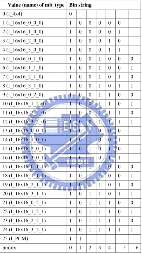
All formats of the binarization coding process are introduced above. But there is still a special coding flow which we don’t describe yet. In order to perform the higher video quality, the macroblock and sub-macroblock are divided into many kinds of types such as I, P, B, and SI slices. In the four basic types, they are also sorted by variable block sizes. These two syntax elements are difficult to define by means of the aforementioned coding flows. In H.264/AVC, it adopts the table-based method to define the macro and sub-macroblock types. The binarization engine reads the bin string and checks if the bin string is mapped the specified location in these tables. If the assigned bin string is found in these tables, it can look up the current macroblock type.

The binarization scheme for coding of macroblock type in I slice is specified in Table 3 [1]. For example, if the value of bin string is equal to “1001011” in I slice, the mapped macroblock type is equal to “8” by look up Table 3. We observe that the probability of the macroblock type appearance is large and its corresponding bin string is shorter.

For macroblock types in SI slices, the binarization consists of bin strings specified as a concatenation of a prefix and a suffix bit string as follows.

The prefix bit string consists of a single bit, which is specified by b0 = ( ( mb_type

= = SI)? 0 : 1 ). For the syntax element value for which b0 is equal to 1, the

binarization is given by concatenating the prefix b0 and the suffix bit string as specified

Table 3 Binarization for macroblock types in I slice Value (name) of mb_type Bin string

0 (I_4x4) 0 1 (I_16x16_0_0_0) 1 0 0 0 0 0 2 (I_16x16_1_0_0) 1 0 0 0 0 1 3 (I_16x16_2_0_0) 1 0 0 0 1 0 4 (I_16x16_3_0_0) 1 0 0 0 1 1 5 (I_16x16_0_1_0) 1 0 0 1 0 0 0 6 (I_16x16_1_1_0) 1 0 0 1 0 0 1 7 (I_16x16_2_1_0) 1 0 0 1 0 1 0 8 (I_16x16_3_1_0) 1 0 0 1 0 1 1 9 (I_16x16_0_2_0) 1 0 0 1 1 0 0 10 (I_16x16_1_2_0) 1 0 0 1 1 0 1 11 (I_16x16_2_2_0) 1 0 0 1 1 1 0 12 (I_16x16_3_2_0) 1 0 0 1 1 1 1 13 (I_16x16_0_0_1) 1 0 1 0 0 0 14 (I_16x16_1_0_1) 1 0 1 0 0 1 15 (I_16x16_2_0_1) 1 0 1 0 1 0 16 (I_16x16_3_0_1) 1 0 1 0 1 1 17 (I_16x16_0_1_1) 1 0 1 1 0 0 0 18 (I_16x16_1_1_1) 1 0 1 1 0 0 1 19 (I_16x16_2_1_1) 1 0 1 1 0 1 0 20 (I_16x16_3_1_1) 1 0 1 1 0 1 1 21 (I_16x16_0_2_1) 1 0 1 1 1 0 0 22 (I_16x16_1_2_1) 1 0 1 1 1 0 1 23 (I_16x16_2_2_1) 1 0 1 1 1 1 0 24 (I_16x16_3_2_1) 1 0 1 1 1 1 1 25 (I_PCM) 1 1 binIdx 0 1 2 3 4 5 6

In other words, the macroblock in SI slice is the enhanced format of the macroblock type in I slice. The bin string of SI slice macroblock type is composed of

suffix part and the syntax element is equal to 0. If the prefix bit is equal to 1, the suffix part is defined in Table 3 and the mapped value of macroblock types has to be added by 1 in SI slice.

Besides the macroblock type in SI slice, there are still two cases that they generate the bin value through the suffix process. The binarization schemes for P macroblock types in P and SP slices and B macroblocks in B slices are specified in Table 4 [1]. Table 4 is the prefix definitions of mb_type. The suffix parts are decided by the formats in Table 3 because these fields are the intra macroblock type in P, SP, and B slice. But the value of the macroblock type in the last fields in P and B slice have to be added by offset value.

The bin string for I macroblock types in P and SP slices corresponding to mb_type value 5 to 30 consists of a concatenation of a prefix, which consists of a single bit with value equal to 1 as specified in Table 4 and a suffix as specified in Table 3, indexed by subtracting 5 from the value of my_type. Namely in the P and SP slices, the value of mb_type is equal to the summation of the offset value “5” and the corresponding value of mb_type for current bin string in Table 3 if the prefix bit of the current bin string is equal to “1”.

The bin string for I macroblock types in B slices (mb_type values 23 to 48) the binarization consists of bin strings specified as a concatenation of a prefis bit string as specified in Table 4 and the suffix bit strings as specified in Table 3, indexed by subtracting 23 from the value of mb_type. Namely in the B slices, the value of mb_type is equal to the summation of the offset value “23” and the corresponding value of mb_type for current bin string in Table 3 if the prefix bits of the current bin string is equal to “111101”.

Table 4 Binarization for macroblock types in P, SP, and B slices Slice type Value (name) of mb_type Bin string

0 (P_L0_16x16) 0 0 0 1 (P_L0_L0_16x8) 0 1 1 2 (P_L0_L0_8x16) 0 1 0 3 (P_8x8) 0 0 1 4 (P_8x8ref0) na P, SP slice

5 to 30 (Intra, prefix only) 1

0 (B_Direct_16x16) 0 1 (B_L0_16x16) 1 0 0 2 (B_L1_16x16) 1 0 1 3 (B_Bi_16x16) 1 1 0 0 0 0 4 (B_L0_L0_16x8) 1 1 0 0 0 1 5 (B_L0_L0_8x16) 1 1 0 0 1 0 6 (B_L1_L1_16x8) 1 1 0 0 1 1 7 (B_L1_L1_8x16) 1 1 0 1 0 0 8 (B_L0_L1_16x8) 1 1 0 1 0 1 9 (B_L0_L1_8x16) 1 1 0 1 1 0 10 (B_L1_L0_16x8) 1 1 0 1 1 1 11 (B_L1_L0_8x16) 1 1 1 1 1 0 12 (B_L0_Bi_16x8) 1 1 1 0 0 0 0 13 (B_L0_Bi_8x16) 1 1 1 0 0 0 1 14 (B_L1_Bi_16x8) 1 1 1 0 0 1 0 15 (B_L1_Bi_8x16) 1 1 1 0 0 1 1 16 (B_Bi_L0_16x8) 1 1 1 0 1 0 0 17 (B_Bi_L0_8x16) 1 1 1 0 1 0 1 18 (B_Bi_L1_16x8) 1 1 1 0 1 1 0 19 (B_Bi_L1_8x16) 1 1 1 0 1 1 1 20 (B_Bi_Bi_16x8) 1 1 1 1 0 0 0 21 (B_Bi_Bi_8x16) 1 1 1 1 0 0 1 22 (B_8x8) 1 1 1 1 1 1 B slice

23 to 48 (Intra, prefix only) 1 1 1 1 0 1

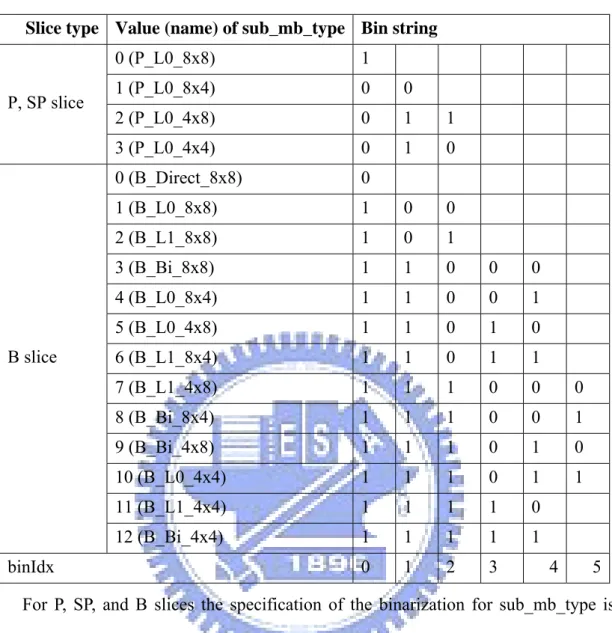
Table 5 Binarization for sub-macroblock types in P, SP, and B slices Slice type Value (name) of sub_mb_type Bin string

0 (P_L0_8x8) 1 1 (P_L0_8x4) 0 0 2 (P_L0_4x8) 0 1 1 P, SP slice 3 (P_L0_4x4) 0 1 0 0 (B_Direct_8x8) 0 1 (B_L0_8x8) 1 0 0 2 (B_L1_8x8) 1 0 1 3 (B_Bi_8x8) 1 1 0 0 0 4 (B_L0_8x4) 1 1 0 0 1 5 (B_L0_4x8) 1 1 0 1 0 6 (B_L1_8x4) 1 1 0 1 1 7 (B_L1_4x8) 1 1 1 0 0 0 8 (B_Bi_8x4) 1 1 1 0 0 1 9 (B_Bi_4x8) 1 1 1 0 1 0 10 (B_L0_4x4) 1 1 1 0 1 1 11 (B_L1_4x4) 1 1 1 1 0 B slice 12 (B_Bi_4x4) 1 1 1 1 1 binIdx 0 1 2 3 4 5

For P, SP, and B slices the specification of the binarization for sub_mb_type is given in Table 5. Instead of looking up the prefix part in one table and looking up the suffix part in other table, it only takes Table 5 to process the binarization of sub-macroblock types in P, SP, and B slices.

2.3 Algorithm of basic binary arithmetic coding

In this section, we introduce the basic arithmetic encoding and decoding algorithm to understand the organization of the arithmetic code. It is the basic concept to the advanced binary arithmetic algorithm in Section 2.4.

2.3.1 Basic binary arithmetic encoding algorithm

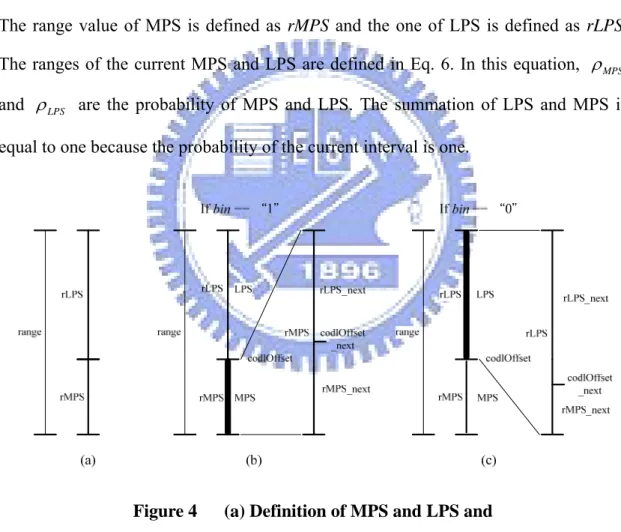
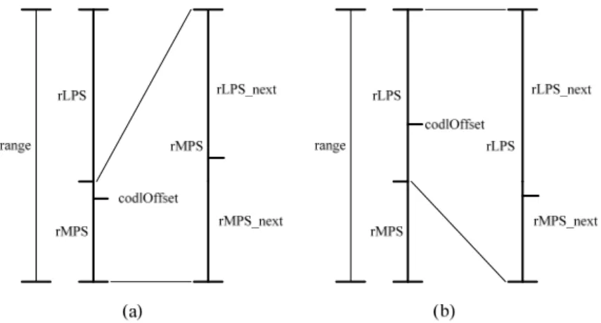
This section introduces the basic arithmetic encoding algorithm to understand the binary arithmetic coding algorithm and know how to decode the bit-stream which is generated by encoder. According to the probability, the binary arithmetic encode defines two sub-intervals in the current range. The two sub-intervals are named as MPS (Most Probable Symbol) and LPS (Least Probable Symbol). Figure 4(a) shows the definition of the sub-intervals. The lower part is MPS and the upper one is LPS. The range value of MPS is defined as rMPS and the one of LPS is defined as rLPS. The ranges of the current MPS and LPS are defined in Eq. 6. In this equation, ρMPS

and ρ_LPS are the probability of MPS and LPS. The summation of LPS and MPS is equal to one because the probability of the current interval is one.

Figure 4 (a) Definition of MPS and LPS and

(b) Sub-divided interval of MPS and

(1 ) MPS LPS MPS rMPS range rLPS range range ρ ρ ρ = × = × = × − : MPS ρ The probability of MPS : LPS

ρ The probability of LPS (Eq. 6)

Depending on the bin decision, it identifies as either MPS or LPS. If bin is equal to “1”, the next interval belongs to MPS. Figure 4(b) shows the MPS sub-interval condition and the lower part of the current interval is the next one. The range of the next interval is re-defined as rMPS and ρMPSis increased. On the contrary, the next

current interval belongs to LPS when bin is equal to “0”. Figure 4(c) shows the LPS sub-interval condition and the upper part of the current interval is the next one. The range of the next interval is re-defined as rLPS and ρ_MPSis decreased.

We arrange the algorithm in the following Eq. 7 and Eq. 8.

Most probable symbol (MPS) condition:

The MPS probability of the next interval:ρ_{MPS_NEXT} =ρ_MPS +ρ_Inc The range of the next interval: range_NEXT =rMPS

The value of the next interval: codlOffsetNEXT =rMPS×ρMPS_{_}NEXT Inc

ρ : The increment of ρMPS. (Eq. 7)

Least probable symbol (LPS) condition:

The MPS probability of the next interval:ρ_{MPS_NEXT} =ρ_MPS −ρ_Dec The range of the next interval: range_NEXT =rLPS

The value of the next interval: codlOffsetNEXT =codlOffset+rLPS×ρMPS_{_}NEXT Dec

codlOffset is allocated at the intersection between the current MPS and LPS range. Depending on codlOffset, the arithmetic encoder produces the bit-stream in order to achieve the compression effect.

2.3.2 Basic binary arithmetic decoding algorithm

In the binary arithmetic decoder, it decompresses the bit-stream to the bin value which offers the binarization to restore the syntax elements. The decoding process is similar to the encoding one. Both of them are executed by means of the recursive interval subdivision. But they still have some different coding flow, which is described as follows.

It is needed to define the initial range and the MPS probability ρ_MPS when starting the binary arithmetic decode. The value of codlOffset is composed of the bit-stream and compared with rMPS. The MPS and LPS conditions are unlike the definitions of the encoder. Figure 5 illustrates the subdivision of the MPS and LPS condition. If codlOffset is less than rMPS, the condition belongs to MPS. The range of the next interval is equal to rMPS. The probability of MPS (ρMPS) is increased and

the bin value outputs “1”. The next value of codlOffset remains the current one. Figure 5(a) illustrates the MPS condition. If codlOffset is great than or equal to rMPS, the next interval turns into LPS. The range of the next interval is defined as rLPS. The probability of MPS (ρMPS) is decreased and the bin value outputs “0”. The meaning

of the next value of codlOffset is to subtract the rMPS from the current codlOffset. Figure 5(b) illustrates the MPS condition.

Figure 5 (a) Result of MPS subdivision and

(b) Result of LPS subdivision

We arrange the algorithm in the following Eq. 9 and Eq. 10.

Most probable symbol (MPS) condition: If ( codlOffset < rMPS )

The bin Value = “1”

The value of the next codlOffset: codlOffset_NEXT =codlOffset The MPS probability of the next interval:ρMPS_{_}NEXT =ρMPS +ρInc

The range of the next interval: rangeNEXT =rMPS Inc

ρ : The increment of ρ_MPS. (Eq. 9)

Least probable symbol (LPS) condition: If( codlOffset >= rMPS )

The value of the next codlOffset: codlOffsetNEXT =codlOffset−rMPS

The MPS probability of the next interval:ρ_{MPS_NEXT} =ρ_MPS −ρ_Dec The range of the next interval: range_NEXT =rLPS

Dec

2.4 Advanced binary arithmetic coding for

H.264/AVC

According to the H.264/AVC standard [1], we introduce the advanced binary arithmetic algorithm adopted by CABAC in this section. It makes more efficient with the integer operation for range computation by means of multiplication-free and table-based probability architecture.

2.4.1 Advanced binary arithmetic encoding algorithm

In Section 2.3.1, we introduce the basic algorithm of the binary arithmetic encode. Although it can achieve the high compression gain, the algorithm works under the floating-point operation. The hardware complexity becomes the problem when we implement the binary arithmetic encoder. In Eq. 6, it has to compute the values of rMPS and rLPS with two multipliers and processes the next value of codlOffset, range, and the probability by means of the floating adders and comparators. It consumes the lots hardware cost because the multipliers and floating operations make the complex circuit. According to H.264/AVC standard [1], we adopt the low complexity algorithm to implement the CABAD circuit.

In order to improve the coding efficiency, there are three kinds of the binary arithmetic decoders in H.264/AVC system such as the normal, bypass, and termination encoding flow. We will show whole algorithms as follows.

The first algorithm is the normal encoding process which is shown in Figure 6. There are two main factors to dominate the hardware efficiency. One is the multiplier

asρ_LPS. In Eq. 6, it applies one multiplier to find the range of LPS (rLPS). According to the H.264/AVC standard, the table-based method is used in place of the multiplication operation. In the normal decoding flowchart, codlRangeLPS looks up the table, rangeTabLPS, depending on two indexes such as pStateIdx and qCodlRangeIdx. pStateIdx is defined as the probability of MPS (ρ_MPS) which gets from the context model. qCodlRangeIdx is the quantized value of the current range (codlRange) which is separated to four parts in this table. The second factor of the improved method is to estimate the value of ρMPS. In Section 2.3.1, we know that the

value of ρ_MPS is increased when MPS condition happened and is decreased when LPS condition happened. But we can’t find the rule how much the value has to be increased or decreased.

The flowchart of Figure 6 also shows the table-based method to process the probability estimation. It divides into two sub-intervals such as MPS and LPS conditions. Depending on the sub-interval, it computes the next probability by the transIdxLPS table when the interval division is LPS and by the transIdxMPS table when the interval is MPS. These two probability tables are approximated by sixty-four quantized values indexed by the probability of the current interval.

Figure 7 Flowchart of renormalization in the encoder [1]

In the basic binary arithmetic encoding, the interval subdivision is operated under the floating-point operation. In practical implementation, this method causes the complexity of the circuit to be increased. The advanced algorithm adopts the integer operation for H.264/AVC. The value of the next range becomes smaller than the

and codlLow. Figure 7 shows the flowchart of renormalization in the encoder. The MSB of codlRange always keeps “1” in order to realize the integer operation. If the MSB of codlRagne is equal to “0”, the value of codlRagne has to be shifted left until the current bit is equal to “1”. The codlLow follows the codlRange to shift left synchronously. Depending on the shifted number of codlRagne, it dominates the number of iteration for codlLow compute directly and affects the PutBit procedure indirectly.

Figure 8 Flowchart of PutBit(B) [1]

Figure 8 shows the flowchart of PutBit procedure. It is dominated by the codlLow decision branch and the bitsOutstanding accumulated in renormalization procedure. The codlLow decision branch dominates its leading bit of one piece bit-stream for current codlLow. Besides dominating the leading bit, the codlLow decision branch also controls if the bitsOutstanding should be accumulated. The accumulated bitsOutstanding dominates the number of bit will be generated in one piece bit-stream for current codlLow. For example, if the current codlLow is 01_xxxx_xxxx, and the current accumulated bitsOutstanding is 5, the bit-stream will not be generated. Instead

of generating bit-stream, the bitsOutstanding will be added 1. So the next bitsOutstanding is 6. If the current codlLow is 11_xxxx_xxxx, and the current accumulated bitsOutstanding is 5, the generated bit-stream in PutBit procedure is 10_0000. The length of the generated bit-stream is variable decided by the accumulated value of bitsOutstanding. The accumulation of bitsOutstanding restricts the throughput of the whole arithmetic encoder. The proposed method of lowering its affection in throughput will be introduced in Chapter 3. Besides, the accumulation of bitsOutstanding also leads to the large range in the length of generated variable bit-stream. It causes the cost issue in output interface design. The proposed method of cost efficiency in output interface will also be introduced in Chapter 3.

The second algorithm is the bypass encoding process which is applied by the specified syntax elements such as abs_mvd, significant_coeff_flag, last_significant_coeff_flag, and coeff_abs_level_minus1. The probabilities of MPS and LPS are fair; therefore, both probabilities are 0.5. It is unnecessary to refer to the context model during decoding. Figure 9 shows the flowchart of the bypass encoding flow. Compared with Figure 6, the bypass encoding process doesn’t estimate the probability of the next interval. So we don’t see the probability computation in the bypass encoding. The computed codlRange doesn’t change which means that it has no renormalization in the bypass decoding. But the codlLow decision branch in bypass encoding is similar to the one in renormalization, so we can modify it to be hardware sharing with renormalization in hardware implementation. Besides, it just uses one adder and one no iteration renormalization to implement the encoding process. So we will adopt the multi-symbol architecture based on the result of statistic in several image test sequences to speed up the throughput of the CABAC system due to its simple process. The proposed multi-symbol architecture will be shown in Chapter 3.

The third algorithm is the termination encoding process. Figure 10 shows the flowchart of the terminal encoding flow. The terminal encoding process is simple as well, but it has the more encoding procedure compared to the bypass encoding process. It doesn’t need the context model to refer to the probability. No matter the subdivision condition belongs to MPS or LPS, the value of the next codlRange is always to subtract two from the current codlRange at first. When the subdivision condition is LPS, the EncodeFlush process shown at figure 11 has to be executed. The purpose of EncodeFlush is stuffing several bits to divide the bit-stream of current macroblock and the bit-stream of next macroblock. In the EncodeFlush process, the codlRange is always assigned to be the constant value which is two at first. For whole termination process, both MPS process and LPS process have to execute renormalization process. In the MPS process, it only executes the renormalization process. In the LPS process, it has to perform two steps process. The first step is to update the codlLow value by taking original codlLow to add the initial codlRange which has been subtracted two.

The termination process occurs one time per macroblock encoding process, it is seldom used during all encoding processes. Therefore, it affects slightly in the throughput of whole CABAC encoding system. So we will focus on the first two algorithms in this section.

2.4.2 Advanced binary arithmetic decoding algorithm

In Section 2.3.2, we introduce the basic algorithm of the binary arithmetic decode. The drawbacks of it is the same as the basic algorithm of the binary arithmetic encode, it also leads to more complexity in hardware implementation due to the multipliers and floating-point operations. As arithmetic algorithm used in CABAC encoding, the arithmetic decoding also adopts three kinds of decoding modes such as the normal, bypass, and termination decoding flow to lower its complexity in circuit implementation. We will show these three decoding algorithms as follows.

The first algorithm is the normal decoding process which is shown in Figure 12. As advanced binary arithmetic encoding algorithm, there are also two main factors to dominate the hardware efficiency for the advanced binary arithmetic decoding algorithm. One is the multiplier of range×ρ_LPS defined as rLPS and the other is the probability calculation defined asρLPS. In Eq. 6, it applies one multiplier to find the

range of LPS (rLPS). According to the H.264/AVC standard, the table-based method is used in place of the multiplication operation. In the normal decoding flowchart, codlRangeLPS looks up the table, rangeTabLPS, depending on two indexes such as pStateIdx and qCodlRangeIdx. pStateIdx is defined as the probability of MPS (ρ_MPS) which gets from the context model. qCodlRangeIdx is the quantized value of the current range (codlRange) which is separated to four parts in this table. The second factor of the improved method is to estimate the value of ρ . In Section 2.3.2, we

know that the value of ρ_MPS is increased when MPS condition happened and is decreased when LPS condition happened. But we can’t find the rule how much the value has to be increased or decreased. The flowchart of Figure 12 also shows the table-based method to process the probability estimation. It divides into two sub-intervals such as MPS and LPS conditions. Depending on the sub-interval, it computes the next probability by the transIdxLPS table when the interval division is LPS and by the transIdxMPS table when the interval is MPS. These two probability tables are approximated by sixty-four quantized values indexed by the probability of the current interval.

codIOffset >= codIRange

binVal = !valMPS codIOffset = codIOffset - codIRange

codIRange = codIRangeLPS binVal = valMPS pStateIdx = transIdxMPS[pStateIdx] Yes No RenormD Done DecodeDecision (ctxIdx)

qCodIRangeIdx = (codIRange>>6) & 3 codIRangeLPS = rangeTabLPS[pStateIdx][qCodIRangeIdx]

codIRange = codIRange - codIRangeLPS

pStateIdx == 0?

valMPS = 1 - valMPS

pStateIdx = transIdxLPS[pStateIdx]

Yes

No

the floating-point operation. In practical implementation, this method causes the complexity of the circuit to be increased. The advanced algorithm adopts the integer operation for H.264/AVC. The value of the next range becomes smaller than the current interval. So we use the renormalization method to keep the scales of codlRange and codlOffset. Figure 13 shows the flowchart of renormalization. The MSB of codlRange always keeps “1” in order to realize the integer operation. If the MSB of codlRagne is equal to “0”, the value of codlRagne has to be shifted left until the current bit is equal to “1”. Depending on the shifted number of codlRagne, codlOffset fill the bit-stream in the LSB.

Figure 13 Flowchart of renormalization in the decoder [1]

The second algorithm is the bypass decoding process which is applied by the specified syntax elements such as abs_mvd, significant_coeff_flag, last_significant_coeff_flag, and coeff_abs_level_minus1. The probabilities of MPS and LPS are fair, that is, both probabilities are 0.5. It is unnecessary to refer to the context model during decoding. Figure 14 shows the flowchart of the bypass decoding flow.

Compared with Figure 12, the bypass decoding process doesn’t estimate the probability of the next interval. So we can’t see the probability computation in the bypass decoding. The computed codlRange doesn’t change which means that it has no renormalization in the bypass decoding. It just uses one subtraction to implement this decoding process. This algorithm is very simple, so we will use the architecture to speed up the CABAD system.

Figure 14 Flowchart of the bypass decoding flow [1]

codIOffset >= codIRange binVal = 1 binVal = 0 Yes No Done DecodeTerminate RenormD codIRange = codIRange-2

Figure 15 Flowchart of the terminal decoding flow [1]

as well, but it has the more decoding procedure compared to the bypass decoding process. It doesn’t need the context model to refer to the probability. The value of the next codlRange is always to subtract two from the current codlRange depending on whether the subdivision condition belongs to MPS or not. The final values of codlRange and codlOffset are required to renormalize through the RenormD in this figure when it branches to the situation that codlOffset is smaller than codlRange (MPS condition). The architecture of this flowchart is composed of one constant subtraction, one comparator, and one renormalization. The termination decoding process is used to trace if the current slice is ended. It occurs one time per macroblock process which is seldom used during all decoding processes.

2.5 Context model organization

The values of the context model offer the probability value of MPS (pStateIdx) and the historical value of bin (MPS) in order to achieve the adaptive performance. The number of the context model is 399 for baseline profile and 701 for main profile. Here we take the baseline profile context model to introduce the operation of the context model briefly. In the normal encoding/decoding process of the arithmetic encoder/decoder, we have to prepare the 399 locations of the context model to record all encoding/decoding results.

context model index = ctxIdxOffset+ctxIdxInc (Eq. 11) context model index = ctxIdxOffset+ ctxIdxBlockCatOffset+ ctxIdxInc (Eq. 12) We divide into two kinds of the context model index methods to allocate the context model. Eq. 11 is one of the index methods. Except residual data encoding/decoding, the context model index is equal to the sum of ctxIdxOffset and

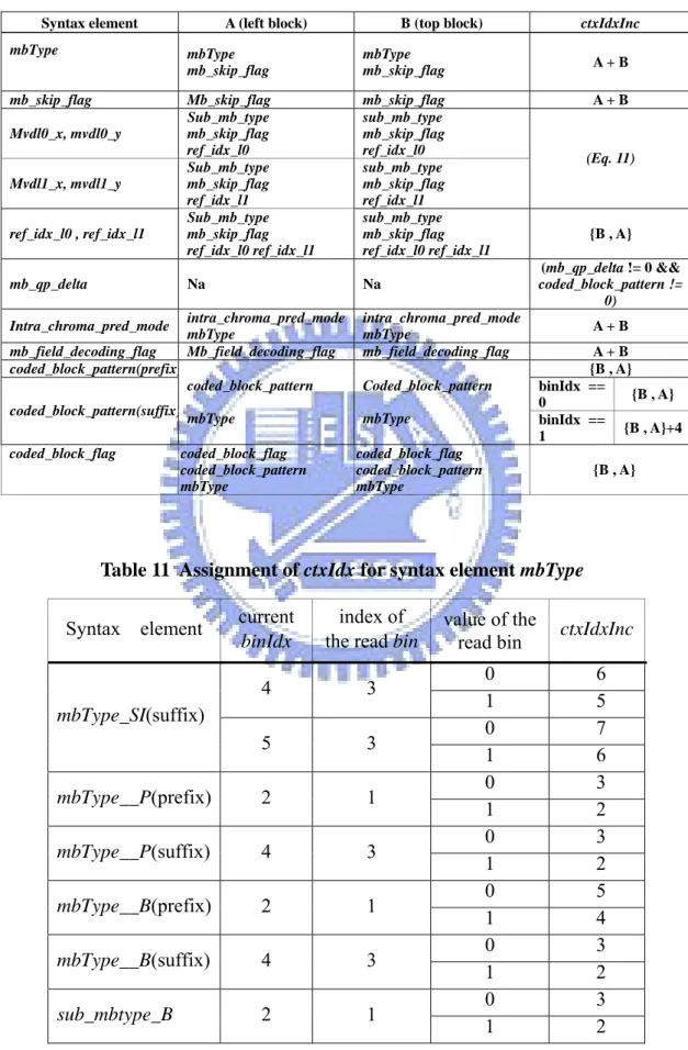
ctxIdxOffset in Table 6. The value of ctxIdxInc is looked up in Table 9 by referring to the syntax element and binIdx. In table 9, the alphabet of “na” denotes the never happened issue and the word of “Terminate” means that the encoding/decoding flow enters the terminal encoding/decoding process. If the generated bin is equal to “1”, the slice has to be stopped and encodes/decodes the next slice. Table 10 shows the value of ctxIdxInc referring to the required neighbor syntax elements of top and left blocks which will be explained in Section 2.6. Table 11 shows the value of ctxIdxInc in special binIdx when encoding/decoding mb_type in Table 9.

Eq. 12 is the index method for the residual data encoding/decoding which focuses on the syntax element of the residual data encoding/decoding flow such as coded_block_flag, significant_coeff_flag, last_significant_coeff_flag, and coeff_abs_level_minus1. The value of the context model index is the sum of ctxIdxOffset, ctxIdxBlockCatOffset, and ctxIdxInc. The assignment of ctxIdxOffset is also shown in Table 6. The value of ctxIdxBlockCatOffset is defined as Table 8 which is dominated by the parameters of syntax elements and ctxBlockCat. The value of ctxBlockCat is the block categories for the different coefficient presentations. maxNumCoeff means the required coefficient number of the current ctxBlockCat. ctxBlockCat sorts five block categories which are luma_DC for 4x4 blocks, luma_AC for 4x4 blocks, luma_4x4, chroma_DC, and chroma_AC in Table 7. The value of ctxIdxInc in residual data is defined as the scanning position that ranges from 0 to “maxNumCoeff – 2” in Table 7. The scanning position of the residual data process has two scanning orders. One is scanned for frame coded blocks with zig-zag scan and the other is scanned for field coded blocks with field scan.

Table 6 Value of ctxIdxOffset definition [1]

slice type image layer syntax element

SI I P,SP B mb_skip_flag ─ ─ 11 24 slice data mb_field_decoding_flag 70 70 70 70 mb_type 3 ─ ─ ─ mb_type(prefix) 0 ─ 14 27 mb_type(suffix) 3 ─ 17 32 coded_block_pattern(prefix) 73 73 73 73 coded_block_pattern(suffix) 77 77 77 77 macroblock layer mb_qp_delta 60 60 60 60 Prev_intra4x4_pre_mode_flag 68 68 68 68 rem_intra4x4_pred_mode 69 69 69 69 MB prediction (intra) Intra_chroma_pred_mode 64 64 64 64 ref_idx_l0 ─ ─ 54 54 ref_idx_l1 ─ ─ ─ 54 Mvd_l0_x ─ ─ 40 40 Mvd_l1_x ─ ─ ─ 40 Mvd_l0_y ─ ─ 47 47 MB prediction and sub-MB prediction (inter) Mvd_l1_y ─ ─ ─ 47

sub-MB prediction sub_mb_type ─ ─ 21 36

coded_block_flag 85 85 85 85 Significant_coeff_flag(field) 105 105 105 105 Significant_coeff_flag(frame) 277 277 277 277 last_significant_coeff_flag(field) 166 166 166 166 last_significant_coeff_flag(frame) 338 338 338 338 residual data Coeff_abs_level_minus1 227 227 227 227

Table 7 Assignment of ctxBlockCat due to coefficient type [1]

coefficient type maxNumCoeff ctxBlockCat

luma DC 16 0

luma AC 15 1

Luma coefficient 16 2

chroma DC 4 3

Table 8 Assignment of ctxIdxBlockCatOffset due to ctxBlockCat and syntax elements of the residual data [1]

ctxBlockCat Syntax element of the residualdata _{0 1 2 3 4} coded_block_flag 0 4 8 12 16 Significant_coeff_flag 0 15 29 44 47 last_significant_coeff_flag 0 15 29 44 47 coeff_abs_level_minus1 0 10 20 30 39

Table 9 Definition of the ctxIdxInc value for context model index [1]

binIdx Syntax element 0 1 2 3 4 5 >=6 mbType_SI(prefix) na na na na na na mbType_SI(suffix) mbType_I Terminate 3 4 5,6 6,7 7 Mb_skip_flag_P 0,1,2 na na na na na na mbType_P(prefix) 0 1 2,3 na na na na mbType_P(suffix) 0 Terminate 1 2 2,3 3 3 sub_mb_type_P 0 1 2 na na na na Mb_skip_flag_B na na na na na na mbType_B(prefix) 0,1,2 3 4,5 5 5 5 5 mbType_B(suffix) 0 Terminate 1 2 2,3 3 3 sub_mbType_B 0 1 2,3 3 3 3 na mvdl0_x, mvdl1_x 3 4 5 6 6 6 mvdl0_y, mvdl1_y 0,1,2 3 4 5 6 6 6 Ref_idx_l0 , ref_idx_l1 0,1,2,3 4 5 5 5 5 5 Mb_qp_delta 0,1 2 3 3 3 3 3 intra_chroma_pred_mode 0,1,2 3 3 na na na na prev_intra4x4_pre_mode_fl _{0 na na na na na na} rem_intra4x4_pred_mode _{0 0 0 na na na na} Mb_field_decoding_flag 0,1,2 na na na na na na coded_block_pattern(prefix) 0,1,2,3 0,1,2,3 0,1,2,3 na na na coded_block_pattern(suffix) 0,1,2,3 4,5,6,7 na na na na na 0 na na na na na na

Table 10 Required syntax elements of the left and top neighbor blocks and the computation for ctxIdxInc

Syntax element A (left block) B (top block) ctxIdxInc mbType _mbType

mb_skip_flag

mbType

mb_skip_flag A + B mb_skip_flag Mb_skip_flag mb_skip_flag A + B

Mvdl0_x, mvdl0_y Sub_mb_type mb_skip_flag ref_idx_l0 sub_mb_type mb_skip_flag ref_idx_l0 Mvdl1_x, mvdl1_y Sub_mb_type mb_skip_flag ref_idx_l1 sub_mb_type mb_skip_flag ref_idx_l1 (Eq. 11) ref_idx_l0 , ref_idx_l1 Sub_mb_type mb_skip_flag ref_idx_l0 ref_idx_l1 sub_mb_type mb_skip_flag ref_idx_l0 ref_idx_l1 {B , A} mb_qp_delta Na Na (mb_qp_delta != 0 && coded_block_pattern != 0) Intra_chroma_pred_mode intra_chroma_pred_mode mbType intra_chroma_pred_mode mbType A + B mb_field_decoding_flag Mb_field_decoding_flag mb_field_decoding_flag A + B

coded_block_pattern(prefix) {B , A} binIdx == 0 {B , A} coded_block_pattern(suffix) coded_block_pattern mbType Coded_block_pattern mbType binIdx == 1 {B , A}+4 coded_block_flag coded_block_flag coded_block_pattern mbType coded_block_flag coded_block_pattern mbType {B , A}

Table 11 Assignment of ctxIdx for syntax element mbType

Syntax element current binIdx

index of

the read bin value of the read bin ctxIdxInc

0 6 4 3 1 5 0 7 mbType_SI(suffix) 5 3 1 6 0 3 mbType__P(prefix) 2 1 1 2 0 3 mbType__P(suffix) 4 3 1 2 0 5 mbType__B(prefix) 2 1 1 4 0 3 mbType__B(suffix) 4 3 1 2 0 3 sub_mbtype_B 2 1 1 2

In addition, ctxIdxInc related to the syntax element of mvd has the special definition. Eq. 13 shows the ctxIdxInc definition of mvd. It checks the sum of the absolute mvd values in left and top sub-macroblocks. If the summation is less than “3”, the value ctxIdxInc is defined as “0”. If the summation is greater than “32”, the value ctxIdxInc is defined as “2”. Otherwise, the value ctxIdxInc is defined as “1”.

sum_A_B = abs(mvd[A])+ abs(mvd[B]) If ( sum_A_B < 3)

ctxIdxInc = 0 ; else if( sum_A_B > 32)

ctxIdxInc = 2 ; else

ctxIdxInc = 1 ; (Eq. 13)

2.6 Syntax elements for the neighbor blocks

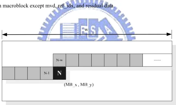
In the previous section, we have explained the methods to compute the context model index to offer the arithmetic decoder to produce the bin value. In both the residual data and the general encoding/decoding, the context model index is dominated by two factors such as ctxIdxOffset and ctxIdxInc. ctxIdxInc is the only one factor related with the syntax elements of the neighbor blocks. In Table 10, we observe the variable syntax elements referring to the left and top blocks to define the ctxIdxInc of the first binIdx such as mb_Type, mb_skip_flag, ref_idx, mb_qp_delta, intra_chroma_pred_mode, mb_field_decoding_flag, and coded_block_pattern. In this section, we introduce how to refer to syntax elements of the left and top neighbor blocks.