行政院國家科學委員會專題研究計畫 成果報告
應用空載雷射掃描系統推估森林結構特性之研究
計畫類別: 個別型計畫 計畫編號: NSC92-2313-B-004-001- 執行期間: 92 年 08 月 01 日至 93 年 07 月 31 日 執行單位: 國立政治大學地政學系 計畫主持人: 詹進發 計畫參與人員: 施瑩瑄、詹凱軒、廖健智 報告類型: 精簡報告 處理方式: 本計畫可公開查詢中 華 民 國 93 年 11 月 2 日
行政院國家科學委員會專題研究計畫期末報告
應用空載雷射掃描系統推估森林結構特性之研究
Estimation of Forest Structural Characteristics Using Airborne Lidar
計畫編號:NSC 92-2313-B-004-001
執行期限:92 年 8 月 1 日至 93 年 7 月 31 日
主持人:詹進發([email protected]) 國立政治大學地政學系
計畫參與人員:施瑩瑄(國立台灣大學森林學系);詹凱軒、廖健智(國立
政治大學地政學系)
摘要 森林之組成與垂直結構提供了重要的 資訊,有助於了解森林生態系之生態狀態 與過程,近年來光達技術的發展,促進了 應用光達於調查森林植被結構之研究。本 研究之目的為發展應用雷射掃描儀獲取林 分結構特性之方法,使用之資料為利用 Leica ALS40 掃 描 闊 葉 樹 林 所 產 生 的 資 料。為了評估光達用於估測林分之植被高 度的能力,本研究以光達資料萃取出表面 高程模型與地形高程模型,並將其與航測 方法所產生的表面高程模型及 4 公尺的地 形高程模型做比較。林分植被高度模型以 表面高程模型與地形高程模型之差表示 之,本研究亦將光達與航測兩者所產生之 植被高度模型作一比較。研究結果顯示, 光達可提供深具價值之量測數據以供推估 植被高度。 關鍵詞:光達,航空測量、表面高程模型、 地形高程模型、森林植被高度 AbstractForest composition and vertical structure provide essential information for understanding the ecological state and process in forest ecosystems. Recent development of lidar technologies has led to
applications of lidar in forest canopy structure investigation. The objective of this study was to develop a method to derive forest stand structure characteristics from laser scanning instrument. Lidar data, acquired using Leica ALS40 airborne laser scanner, of a deciduous forest was used in this study. In order to assess the capability of lidar for estimating canopy height of forest stands, surface and terrain elevation model derived from lidar data were compared to the surface elevations generated using photogrammetric technique and a 4-meter digital elevation model. In addition, the forest canopy height model, represented by the difference of the surface elevation model and terrain elevation model, was compared to measurements from the photogrammetric process. The results indicate that lidar can provide valuable measurements for estimation of forest canopy height.
Keywords: Lidar, photogrammetry, surface elevation model, terrain elevation model, forest canopy height.
1. INTRODUCTION
Forest ecosystem management depends
2
on vast amount of qualitative and quantitative information spanning over different spatial and temporal scales. Obtaining the required information through ground investigation is not feasible because it is too costly in terms of time, manpower, and cost. Consequently, remote sensing techniques have been successfully used in many applications such as forest resources inventory, landscape change detection, natural hazard investigation, and forest biomass estimation (Brown de Colstoun et al., 2003; Haara and Haarala, 2002; Viedma et al., 1997; Wulder, 1998; Wulder et al., 2004).
Despite the remarkable advances of remote sensing technologies in improvement of spectral and spatial resolutions in recent years, the capabilities of the sensors in measuring forest height characteristics were still very limited. Similar to radar, lidar (LIght Detection And Ranging) is a very advanced active remote sensing technique with laser light as the energy source. Lidar obtains measurements at very high density, therefore it provides excellent horizontal resolution. Lidar has the capability of recording multiple return pulses of the initial laser energy. Classification of the return pulses yields both the ground elevation and non-ground elevation, which allows direct measurements of the heights of buildings and vegetation. Recent development of lidar technologies has led to applications of lidar in a variety of research topics such as forest canopy structure investigation, biomass estimation, and forest fire detection (Drake et al., 2002; Hudak et al., 2002; Wehr and Lohr, 1999; Lim and Treitz, 2002; Utkin et al., 2002).
This research utilized an airborne lidar
system for surveying the Yangmingshan National Park area, and the techniques for deriving digital surface model and digital elevation model using lidar was investigated. In addition, the lidar measurements were used to measure canopy heights. To assess the capability of lidar in estimation of forest canopy height, the height measurements were compared to the results generated from photogrammetric procedures.
2. MATERIALS
2.1 STUDY AREAThe study area for this research is located within the Yangmingshan National Park, a very popular recreation area in the vicinity of Taipei City. The elevation of the park ranges from 200 to 1,120 meters with a total area of 11,455 hectares. Established in 1985, the park features unique volcanic landscape and abundant fauna and flora species. Vegetation of the park can roughly be grouped into three categories, i.e., water plants, grasslands, and forest canopy. Growing in water and land environments, there are more than 1,200 plant species, of which several are endemic species. Silvergrass (Miscanthus floridules) and arrow bamboo (Sinobambusa kunishii) often grow
in grasslands, and the forest canopy is primarily composed of broad-leaved tree species, among them the Lauraceae family are dominant species, such as the red nanmu
(Machilus thunbergii) and the large-leaved
nanmu (Machilus kusanoi).
2.2 LIDAR DATA
The lidar data for the study area were acquired using a Leica ALS40 airborne laser
3
scanner mounted on an airplane on April 14, 2002. The sensor was equipped with an aircraft position and orientation system (POS) which recorded the aircraft position and attitude information using a GPS receiver and IMU (inertial measurement unit). The POS data were processed using proprietary software to generate WGS84 ground coordinates of all reflected laser pulses (Leica ). Furthermore, the data were transformed from WGS84 to local coordinate system and subsequently a filtering process was performed to separate ground points from non-ground points. The flight parameters and the number of points in the lidar dataset provided by the vendor are shown in Table 1. Flying height 1,200-2,200 m AGL FOV 35° Scan rates 29.4 Hz Pulse rates 38 KHz All points 22,734,756 Surface points 15,892,054 Ground points 1,686,303
Table 1. Flight parameters and number of points in the lidar dataset
2.3 AERIAL PHOTOGRAPHS
Aerial photographs taken on 12 March 2002 were acquired for this study. The aerial photographs were taken in two flight lines using normal color films with a nominal scale of approximately 1/22,000. These aerial photographs were scanned and converted into digital format with 21 μ m per pixel
resolution. Imageries of the aerial photographs were used to interpret land cover types and to produce DSM (digital surface model) for the study area using digital photogrammetric procedures. Characteristics of aerial photographs and flight parameters are shown in Table 2.
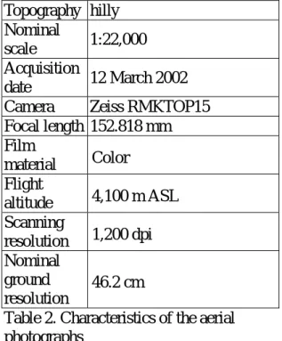
Topography hilly Nominal
scale 1:22,000 Acquisition
date 12 March 2002
Camera Zeiss RMKTOP15 Focal length 152.818 mm Film material Color Flight altitude 4,100 m ASL Scanning resolution 1,200 dpi Nominal ground resolution 46.2 cm
Table 2. Characteristics of the aerial photographs
2.4 SATELLITE IMAGES
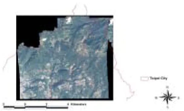
QuickBird satellite images, provided by DigitalGlobe Inc., acquired on 15 December 2002 (path/row = ) were obtained for the study area. The spatial resolution for the panchromatic and multispectral images are 0.7m and 2.8m, respectively. Technical data of the satellite images are listed in Table 3. The satellite images were used for interpretation of land cover types in order to select appropriate sample areas for further investigation.
2.5 DEM
A digital elevation model with resolution of 4 meter was used in this study.
4
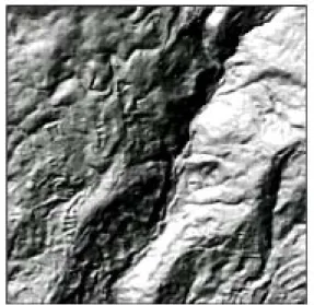
Figure 1 depicts shaded relief of the study area computed from the DEM assuming 315° (azimuth) and 45° (altitude) as the position of the illumination source.
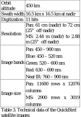
Orbit
altitude 450 km
Swath width 16.5 km x 16.5 km at nadir Digitization 11 bits Resolution Pan: 61 cm (nadir) to 72 cm (25° off-nadir) MS: 2.44 m (nadir) to 2.88 m (25° off-nadir) Image bands Pan: 450 – 900 nm Blue: 450 – 520 nm Green: 520 – 600 nm Red: 630 – 690 nm Near IR: 760 – 900 nm Image size Pan: 11600 rows x 12076 columns MS: 2900 rows x 3019 columns
Table 3. Technical data of the QuickBird satellite images
Figure 1. Shaded relief of the study area produced from DEM
3. METHODS
3.1 PROCESSING OF THE DEMThe DEM was in ARC/INFO GRID format with cell size of 4 meters. Originally, the values of DEM cells were elevation
above the geoid, and the coordinate system was TWD67. Elevation values of the lidar data set were geodetic height, and the coordinate system was WGS84, which is similar to TWD97. In order to compare with lidar data, geoidal undulation of each DEM cell was calculated, and subsequently the DEM was transformed to TWD97 with elevations representing geodetic height. In addition to the DEM, all the other ancillary data, including various vector and raster maps, were transformed to TWD97 such that they could be overlaid with DEM and lidar data. The DEM was used as the reference for ground elevation model, with which the ground elevation model resulted from lidar data was compared.
3.2 PROCESSING OF THE SATELLITE IMAGES
The satellite images were QuickBird Standard Imagery bundled with both panchromatic and multispectral images in GeoTIFF format. Processed by the vendor, the Standard Imagery was normalized for topographic relief with respect to the reference ellipsoid using a coarse DEM. However, only minimal normalization was done and for high relief areas terrain corrections must be applied in order to achieve better accuracy (DigitalGlobe, 2004). The coordinate system of the imageries were UTM zone 51. To have a common coordinate system with the other data, by using PCI Geomatica OrthoEngine, the imageries were orthorectified using ground control points obtained from orthoimages and topographic maps. Figure 2 shows the multispectral image acquired for this study.
5
Figure 2. QuickBird multispectral image
3.3 PROCESSING OF THE LIDAR DATA The lidar data sets contain irregularly spaced points with four measurement readings, i.e., easting, northing, elevation, and intensity of the returned pulse. The data points were collected in across-track scanning pattern, with density of approximately 0.5 pts/m2. In order to compare with the DEM, the data sets were converted to ARC/INFO GRID raster map with common origin and cell size as the DEM. Processing of the lidar data requires large amount of computer disk space and memory because the size of the original data is quite large (812 MB). To reduce processing time, a subset of the lidar data set, 1 km x 1 km, was selected to experiment with the analytical methods developed for this study. The entire lidar data and the location of the subset are shown in Figure 3.
Figure 3. Lidar data and location of the subset
The lidar canopy height model (CHM) was obtained by subtracting the lidar ground elevation model (GEM) from the lidar surface elevation model (SEM). By using software programs written in C and AML (Arc Macro Language), the lidar data set were converted into ARC/INFO point coverages. Moreover, the minimum elevation, maximum elevation, average elevation, and number of points within each grid cell were computed and corresponding GRID maps were created.
3.4 PROCESSING OF AERIAL PHOTOS Aerial photos, in digital format, were processed using Intergraph ImageStation digital photogrammetric workstation. Ground control points used in the photogrammetric process were measured using GPS RTK.
4. RESULTS AND DISCUSSIONS
4.1 DSM GENERATED FROM AERIAL PHOTOSTo compare with the lidar canopy height model, a DSM (digital surface model) with 4-meter resolution was generated by automatching technique. The (X,Y,Z) data were then converted into ARC/INFO grid map using a C program.
4.2 OBSERVATIONS FROM THE LIDAR DATA
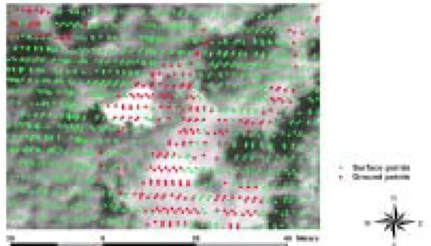
Two types of maps were produced from the lidar data set, i.e., ARC/INFO vector coverages and raster grids. Figure 4 depicts the lidar data classified as surface and ground points overlaid on top of the satellite image. As shown in Figure 4, the amount of surface points was much larger than the ground points. The ground points mostly
6
appeared in roads, building structures, and areas with sparse vegetation, and only small number of them appeared in densely vegetated areas. Figure 5 shows a closer look of these points. The lidar sensor collects data by scanning objects on the ground in a direction perpendicular to the flight direction. Apparently, the horizontal distance between adjacent points on the same scan line were mostly less than 2 meters, with very few of them separated more than 3 meters apart. Along the flight direction, two adjacent scan lines were spaced at about 1 meter, followed by another pair of scan lines about 2 meters apart from the previous scan line.
The lidar points were grouped into 4-meter cells, within each cell statistical analysis was performed. Because of the high point density, only very few grid cells were voids, i.e., without any observation of lidar pulses. For the 1 km x 1 km subset, only 15 out of 62,500 cells were voids, which amounted to 99.98% of coverage for 4-meter cells. All the other cells have at least one data point, with a maximum of 166 points, which appeared to be in areas that were overlapped between flight lines. For those cells without any hits, a close-up examination found that these cells were located in the shadow areas blocked by building structures.
Figure 6 shows the surface elevation model represented by the maximum value within each cell. Figure 7 shows the ground elevation model represented by the minimum value in the grid cell. For comparison, the shaded relief of the DSM generated from aerial photos and the DEM are shown in Figure 8 and Figure 9, respectively. We can see that the variation of the lidar ground elevation model is larger than that of the
DEM. Similar patters were observed from both the lidar surface elevation model and DSM generated from aerial photos. However, the lidar surface elevation model appears to have more variation than the DSM.
4.3 CANOPY HEIGHT
The canopy height model was represented by difference between the surface elevation model and the ground elevation model. Figure 10 and Figure 11 show the canopy height model derived from lidar data and DSM, respectively. It appears that the lidar canopy height model have much more details than the canopy height model generated from DSM.
5. CONCLUSIONS
While a more complete analysis is needed to evaluate the accuracy of estimation of forest canopy height, the results indicate that the lidar data have great potential for measuring forest canopy structure directly. Further study will be focused on validation of the predicted lidar canopy height with field survey data, and methodology for integrating remote sensing data with lidar data to improve the accuracy of classification results as well as canopy height estimation.
Figure 4. Satellite image overlaid with points classified as surface and ground points
7
Figure 5. A closer look of Figure 4
Figure 6. Lidar surface elevation model
Figure 7. Lidar ground elevation model
Figure 8. DSM generated from aerial photos
Figure 9. Shaded relief of the DEM
Figure 11. Canopy height model generated from DSM using aerial photos
ACKNOWLEDGEMENTS
The authors would like to thank the Agricultural and Forestry Aerial Survey Institute for providing data, and the National Science Council for providing support for this study. Our gratitude also goes to the Council of Agriculture and Prof. Shih of the National Chiao Tung University for sponsoring and supervising the lidar pilot project, which resulted in data for this study.REFERENCES
Brown de Colstoun, E.C., Story, M.H., Tompson, C., Commisso, K., Smith, T.G., and Irons, J.R., 2003, National Park vegetation mapping using multitemporal Landsat 7 data and a decision tree classifier, Remote Sensing
of Environment, 85, 316-327.
DigitalGlobe, Inc., 2004, QuickBird Imagery Products—Prouduct Guide, Longmont, Colorado.
Drake, J.B., Dubayah, R.O., Clark, D.B., Knox, R.G., Blair, J.B., Hofton, M.A., Chazdon, R.L., Weishampel, J.F., and Prince, S.D., 2002, Estimatioin of tropical forest structural characteristics
using large-footpring LIDAR, Remote
Sensing of the Environment, 79,
305–319.
Haara, A., and Haarala, M., 2002, Tree Species Classification Using Semi-automatic Delineation of Trees on Aerial Images, Scandinavian Journal of Forest Research, 17, 556-565.
Hudak, A. T., Lefsky, M. A., Cohen, W. B., and Berterretche, M., 2002, Integration of lidar and Landsat ETM+ data for estimating and mapping forest canopy height, Remote Sensing of Environment, 82, 397-416.
Lim, K., and Treitz, P., 2002, Estimating aboveground biomass using lidar remote sensing, Proceeding of SPIE’s International Symposium on Remote Sensing, Agia Pelagia, Crete, Greece,
September 23-27, 2002.
Utkin, A.B., Lavrov, A.V., Costa, L., Simoes, F., and Vilar, R., 2002, Detection of small forest fires by lidar, Applied
Physics B, 74, 77-83.
Viedma, O., Melia, J., Segarra, D., and Carcia-Haro, J., 1997, Modeling Rates of Ecosystem Recovery after Fires by Using Landsat TM Data, Remote Sensing of
Environment, 61, 383-398.
Wehr, A., and Lohr U., 1999, Airborne laser scanning—an introduction and overview.
Journal of Photogrammetry & Remote Sensing, 54, 68-82.
Wulder, M.A., 1998, The Prediction of Leaf Area Index from Forest Pologons Decomposed through the Integration of Remote Sensing, GIS, UNIX, and C,
Computers & Geosciences, 24, 151-157.
Wulder, M.A., Kurz, W.A., and Gillis, M., 2004, National lever forest monitoring and modeling in Canada, Progress in
Planning, 61, 365-381.
Yangmingshan National Park, 2004, Looking to the Future,
http://www.ymsnp.gov.tw/HTML/ENGN EW/info/information.htm (accessed 28 April 2004)