具有多項異常原因之 X-bar管制圖經濟設計

國立交通大學

工業工程與管理學系

博士論文

具有多項異常原因之

管制圖經濟設計

Economic Design of Control Chart

for Multiple Assignable Causes

研 究 生 : 蘇珈儀

指導教授 : 彭文理 博士

具有多項異常原因之

管制圖經濟設計

Economic Design of Control Chart

for Multiple Assignable Causes

研 究 生:蘇珈儀 Student：Chia -Yi Su

指導教授：彭文理 博士 Advisor：Dr. W. L. Pearn

國 立 交 通 大 學

工業工程與管理學系

博士論文

A Dissertation Submitted to

Department of Industrial Engineering & Management

College of Management

National Chiao Tung University

in partial Fulfillment of the Requirements

for the Degree of Philosophy

in

Industrial Engineering & Management

April, 2012

Hsinchu, Taiwan, Republic of China

i

具有多項異常原因之

管制圖經濟設計

學生：蘇珈儀 指導教授：彭文理 博士

國立交通大學管理學院

工業工程與管理學系

摘要

本論文主要研究製程異常原因發生為多項異常原因之 管制圖經濟設計。研 究中製程生產方式分為斷續工件生產及連續流動生產兩種；製程失效機構則考慮指 數分配與韋氏分配兩種。根據生產方式及製程失效機構，在論文中共提出二項研究 主題：(1)連續流動生產且製程失效機構屬指數分配之 管制圖經濟設計，(2)斷續 生產且製程失效機構屬韋氏分配之 管制圖經濟設計。 對於這兩種經濟設計模式，我們利用抽樣方法和成本結構來建構損失成本函數， 並在損失成本最小化下來找尋最佳的n(樣本大小)，h (抽樣間隔時間)，k (管制界限 係數)。由於經濟設計模式進行敏感度研究，可以提供管理者或工程師了解輸入參數對 模式的影響。因此，我們也將對最佳的n, h , k 值進行敏感度分析，藉此分析來了 解時間參數或成本參數的變動後，對於最佳n, h , k 值之影響。最後，我們有提 供數值結果並討論之。 除此之外，我們將對多項異常原因下僅一個異常發生之模式和多項異常原因下 有二個異常發生之模式進行比較分析，藉由數值結果可以得知考慮多項異常原因下 有二個異常發生之模式對於降低品質成本和增加其在斷續生產之競爭力是有一個 有用的方法。 關鍵字：經濟設計， 管制圖，多項異常原因，韋氏衝擊模氏，指數衝擊模式，斷 續生產，連續流動生產。

ii

Economic Design of

Control Chart

for Multiple Assignable Causes

Student: Chia-Yi Su Advisors: Dr. W. L. Pearn

Department of Industrial Engineering and Management, College of Management, National Chiao Tung University

Abstract

In this dissertation, we analyze the economic design of x-control charts and

extend the model for the case of multiple assignable causes to allow for the second occurrence of an assignable cause following the first occurrence. In addition, two process failure mechanisms are investigated in different manufacturing environments. One is the Exponential failure mechanism in a continuous flow process and another is the Weibull failure mechanism in a discrete part process.

For those two models, the expected loss-cost functions are established by the sampling scheme and cost structure. Optimal values of the economic design parameters

including the sampling size(n), the sampling intervals (h ) and control limit coefficient

( k ) are determined by minimizing loss-cost functions. Because of sensitivity

investigation on the model with critical input parameters may provide some answers for the model analyst. A sensitivity analysis is provided to discuss how the model can be affected by the time parameters or cost parameters in the investigated model. For illustration purpose, numerical results are also presented.

Subsequently, we perform comparative analysis between the model that once an assignable cause occurs, no further assignable causes will occur and the modified model that allow for the second occurrence of an assignable cause following the first occurrence.

iii

Our numerical investigations showed that a modified model should be helpful in reducing the quality cost and increasing competitiveness in a discrete part process.

Key words: Continuous Flow Process, Discrete Part Process, Economic design,

Exponential shock model, Multiple assignable causes, Weibull shock model, x-control

iv

Preface

The objective of this dissertation is to provide optimal economically-based control charts for use in detecting out-of-control conditions when monitoring continuous flow process or discrete part process.

I wish to express sincere appreciation to my major adviser, Dr. W. L. Pearn, for his guidance, assistance, and encouragement throughout this research and during my doctoral studies. Thanks also to my another adviser, Dr. Y. M. Yang, for his interest and assistance.

I also wish to thank my committee members, Dr. Kai-Bin Huang, Dr. H. W. Su, Dr. Dong-Yuh Yang, for their assistance. Thanks are extended to my sisters for their moral support to give me the opportunity to fulfill this dissertation.

Finally, I wish to dedicated this dissertation to my parents and my husband, Hung-Chia Kuo, for their sacrifice, understanding, encouragement, and love.

v

List of Contents

page Abstract (Chinese)……….. …………...………..……….………... i Abstract (English)………..……….... ………...……… ii Preface………..…………... iv List of Contents………...………... v

List of Tables………..……….... vii

List of Figures………....…. viii

Chapter 1. Introduction………..…...… 1

1.1 Background……….… 1

1.2 Inspection Interval Principle………..…..…... 4

1.3 Literature Review………..…….. 5

1.3.1 Single special cause………...…….. 5

1.3.2 With warning limits………..………... 6

1.3.3 Joint economic designs……….………... 7

1.3.4 Non-Exponential process failure………..………...….. 7

1.3.5 Multiple special causes……….…...….. 9

1.3.6 Continuous flow process………...….... 10

1.4 Problem Statement………...…... 11

1.5 Scope of Dissertation……….……... 14

Chapter 2. Economic Design of x-Control Charts for Discrete Part Weibull Process with Multiple Assignable Causes………... 16

2.1 Definitions, Assumptions and Notations………..………...… 16

2.2 Formulation of the Expected Cycle Length………..….. 19

2.3. Formulation of the Expected Cost Per Cycle………... 25

2.4. Determination of Optimal Design Parameters………... 27

2.5. Comparison with Chen and Yang’s Model……….…..…. 28

Chapter 3. Economic Design of x -Control Charts for Continuous Flow Process with Multiple Assignable Causes……….…………. 31

vi

3.1 Definitions, Assumptions and Notations………...….. 32

3.2 Formulation of the Expected Cycle Length…………..………..… 35

3.3. Formulation of the Loss-Cost Function………..………... 39

3.4. Determination of Optimal Design Parameters………...….... 40

3.5. Sensitivity Analysis……….…….…….. 42

Chapter 4. Conclusions and Future Research………...….……. 47

4.1 Conclusions………. 47

4.2 Future Research……….. 48

vii

List of Tables

page

2.1 The set of cost and probability parameters………... 28 2.2 Optimal design parameters between the modified model and Chen and Yang’s

model at three different prior distributions as  changes………..……… 30

3.1 The reference set of cost and probability parameters………... 42 3.2 Optimum design parameters for model at three different prior distributions…... 44

viii

List of Figures

page

1.1 Sampling method and plotting on x-control charts in a discrete part process...

…………...………..……….………... 12

1.2 The average cycle length for discrete part process………... ………...……… 12

1.3 Sampling method and plotting on x-control charts in a continuous flow process……….. 13

1.4 The average cycle length for continuous flow process………...……….. 13

2.1 The process of Situation 1 for State 2 in a discrete part process……….. 21

2.2 The process of Situation 2 for State 2 in a discrete part process..……… 22

2.3 The process for State 3 in a discrete part process………. 23

3.1 The process of Situation 1 for State 2 in a continuous flow process….……….. 36

3.2 The process of Situation 2 for State 2 in a continuous flow process.………….. 37

1

Chapter 1

Introduction

Control charts are the most theoretical technology in magnificent seven. Control charts are the primary quality improvement tools in statistical process control (SPC), which used to establish and maintain statistical control of manufacturing process. The effective use of control charts are largely dependent upon their design. For this reason given above, control charts are practical subjects and play important roles in SPC. In Section 1.1, we describe the background of the control charts. Section1.2 is devoted to introduce inspection intervals principle. In Section 1.3, we relate our problem to earlier works in the literature. Section 1.4 shows the description of the models in this thesis. At the end of this chapter, the scope of the thesis is presented in Section 1.5.

1.1 Background

The control chart was originated in 1924 by Shewhart [37] as a means to differentiate between the normal, expected random causes and the special or assignable causes of the process variability. In the development of new processes or products, or in the restudy of existing ones, the Shewhart control charts are still the basic tools for

establishing a state of statistical control ( Gibra [17] ). The control chart is an online

control tool used to detect the mean shifts of a process. When a control chart is used

to monitor the process mean, three questions are concerned by the quality control engineers. These are (1) How large a sample should be employed? (2) At what interval should the samples be taken? (3) What multiple of sigma should be used in determining the control limits? ( Duncan [14] ). Selection of these decision variables based on some subjective and/or objective criteria. Shewhart [37] developed the use of 3-sigma control limits as action limits. The justification of 3-sigma limits is based on empirical-economic

2

considerations rather than on a formal statistical basis. Shewhart settled on subgroup

sizes of 4 or 5 for - and -charts and left the quality control engineer or other

personnel. The design can affect the cost, statistical properties, and ultimately user confidence. Cost considerations are important for obvious reasons.

The concept of an economic design was first introduced by Girshick and Rubin [18]. Although the optimal control rules in their model are too complex to have practical value, their work provided the basis for most cost-based models in control chart designs. The

pioneer investigation of the economic design of an -chart was made by Duncan [14].

He formulated an excellent model for the determination of the optimal parameters of an -chart.

However, these reviews are centered on piece part manufacturing. In continuous processes, there is not a well defined production unit. Almost any chemical, petroleum, bulk liquid, or otherwise semi-homogenized product is a case of this kind. The problem is compounded by the fact that the sample may have been taken from a vat or pipeline in

which there is a homogeneous mixture resulting from flow or agitation. To pull

samples instantaneously from a continuous flow process would usually result in ranges of zero, or in the range being an almost pure measure of test variation. Due to the number of such process, there is a need to develop appropriate quality control techniques for continuous flow processes.

Koo and Case [23] first proposed an economic design of control charts for

using in monitoring continuous flow process, where the amount of time the process remains in control can be formulated as exponential distribution. A sampling scheme in a continuous flow process is to take one sample from the process at each sampling time

and then combine analytical results into a subgroup. That is considerably different

3

In practice, many production processes are affected by several assignable causes. Therefore, processes subject to single assignable cause are not common. In such situation, an investigation of the case where there is a multiplicity of assignable causes is therefore desirable. Duncan [15] has generalized his single assignable model to a situation in which there are s assignable causes, however, where different special causes will shift the process mean by different amounts. Duncan’s multiple causes model is divided into two types: Model I presents “a single occurrence” model. It is assumed that once assignable

cause occurs, the process remains in that other assignable causes occur no longer till

assignable cause is detected; Model II presents “double occurrence”. It is assumed

that the model allows for the second occurrence of an assignable cause following the first occurrence.

Many interesting research results are investigated on the process failure mechanism (see Duncan [14,15], Hu [21], Banerjee and Rahin [3]). Past work regarding process failure mechanism may be classified into three categories: (i) Exponential, (ii) Weibull, and (iii) Gamma. The time between occurrences of successive special causes are exponentially distributed with a specified mean value, and thus, a constant failure rate for the process is implied. Banerjee and Rahin [3] pointed out that the use of a constant sampling interval is counterintuitive in the case of a process with an increasing failure rate. A more realistic approach is to shorten the sampling interval because the process deteriorates further as time goes by.

In this thesis, we deal with two process failure mechanisms in different manufacturing environments with multiple assignable causes. One is the Exponential failure mechanism in a continuous flow process and another is the Weibull failure mechanism in a piece-part process. For those two models, the expected loss-cost functions are established by the sampling scheme and cost structure. Optimal values of

4

the economic design parameters including the sampling size(n ), the sampling intervals

(h ) and control limit coefficient ( k ) are determined by minimizing loss-cost functions.

Analytical results for sensitivity analysis are also obtained.

1.2 Inspection interval principle

In this section, we introduce the inspection interval principle ( Banerjee and Rahim [3] ).We attempt to obtain a near-optimal solution by imposing some sort of restriction on the lengths of sampling intervals. In this connection, we note that the uniform sampling intervals for Markovian shock models provide a constant integrated hazard over each interval. Being motivate by this, we propose that the lengths of the sampling intervals should be chosen in such a way that the integrated hazard over each interval should be equal.

The process is monitored by drawing random samples of size n at times

1, 1 2, 1 2 3,

h h h h h h and so on. Where hj is the j th sampling interval. For

convenience, let Wj be the time of the jth sample, 1 , 1, 2,

j

j i i

W h j and W00.

For a non-uniform sampling, the length of the sampling interval hj( j1, 2, ) is

chosen such that the probability of a process shift in an interval, given no shift until the

start of the interval, is constant for all intervals. This amounts to choosing the hj such

that the integrated hazard rate over each interval is constant. Specifically, the hj is

chosen such that

1 1 0 ( ) ( ) , 0, 1, 2, Wj W W j r t dt r t dt j    





(1.1)

and the Weibull hazard rate is defined by

1

( )

r t t . (1.2)

5



1 1



1 ( 1) j h  j  j  h . (1.3)

From the above Equation (1.3), the hj is a non-increasing function of h1. The Wj goes

to infinity as j goes to infinity. That is h1h2h3 and lim j

jW  .

1.3 Literature Review

The pioneer investigation of the economic design of x-control charts was made by

Duncan [14]. He formulated an excellent model for the determination of the optimal

parameters of x-control charts. These parameters ( the sample size, the time interval

between taking successive samples, and the control limits ) were derived to maximize the approximate average net income of a process. He also made a number of specific assumptions. For example, he assumed an exponential time to failure of the process and that the process is subject to the occurrence of an assignable cause of variation which takes the form of a shift, of constant magnitude, in the process mean. The standard deviation is assumed to remain stable. Furthermore, he assumed that the process is not shut down while the search for the assignable cause is in progress. Since the work by Duncan, numerous authors have made a wide variety of changes to Duncan’s modeling assumptions, the distribution of the time of assignable cause, approach, and et al. on their economic design of process control charts. Earlier work in this area was summarized by Montgomery [27] and Vance [40]. Both are excellent references. Several works focusing

on the economic design of control charts will be discussed.

1.3.1 Single special cause

The classical model for the economic design of x-control charts subject to a single

assignable cause was first introduced by Duncan [14]. An approximation to the optimal design was found. Goel, et al. [19] developed an algorithm to find the exact optimal solution of Duncan’s model by computer. Gibra [16] developed a model for the

6

determination of the optimal parameters of x-control charts. He assumed that the sum

of times required to take, inspect a sample, compute and plot a sample average and to discover and eliminate the assignable cause has an Erlangian distribution. In Duncan’s model, the author assumed that the time to discover and eliminate the assignable cause is constant.

Chiu and Wetherill [11] proposed a simple semi-economic scheme for the design of

a control plan using an x-control chart. They simplified the loss-cost function proposed

by Duncan by eliminating some insignificant terms. The essential characteristic of the semi-economic plan is to specify the probability of true alarms at a value of 0.9 or 0.95. They found that of the 25 semi-economic plans 17 were better than Duncan’s approximate plans and the remaining 8 showed a loss-cost within 1.7% above Duncan’s corresponding values.

Lorenzen and Vance [25] provided one unified approach to the economic design of process control charts. They considered a general process model that applied to all control charts. Collani [13] discussed two process control strategies: (1) As soon as one sample average falls outside the control limits, the process is shut down and action is taken to search the assignable cause of variation. (2) The process is shut down in every h hours. The expected cost produced was given as investigating the assignable cause. Tagaras [39] considered the probability of shift, the correlation of process variance and mean, and error of measurement on the optimal design parameters.

1.3.2 Warning limits

Gordon and Weindling [20] presented the economic design of x-control charts

with warning limits. They consider a single assignable cause model, and minimize the long run average cost per good part produced. Chiu and Cheung [10] presented a study

7

-control charts with both warning and action limits, based on a widely studied process model. They assumed that a search for the assignable cause is undertaken when either (1) any point exceeds the action limit, or (2) a run of N points fall between the action and warning limits. The loss-cost function is following Duncan’s [14] arguments with straightforward modifications.

1.3.3 Joint economic designs

Two charts are usually employed together to monitor the process. One is for monitoring the shift in the process mean; the other for monitoring the change in the process variation. In Duncan’s model, the standard deviation is assumed to remain stable.

Saniga [34] was the first to study the joint economic design of and charts in which

Duncan’s [14] approach is not used. He assumed that two shifts can occur during the

production of a specified number of units. Therefore, the parameters of chart are

considered. Saniga [35] also investigated the sensitivity of the economic design to the type of process model using a discrete-time cost model developed by Barker [4]. Furthermore, Saniga [36] was the first considered an application of economic statistical

principle to the joint design of an and charts. The objective is to minimize the

expected total cost per unit time subject to constraints on the Type I error probability, Type II error probability and average time to signal (ATS).

Still another useful paper is that of Rahim, et al. [33]. Their cost model for their

economically-based and variance charts followed the unified approach of Lorenzen

and Vance [40]. The joint and variance charts were compared to and charts.

Results showed that the and variance charts have lower cost and higher power.

1.3.4 Non-Exponential process failure

8

underlying distribution of the process failure mechanism is exponential. That is, the times between occurrences of successive special causes are exponentially distributed with a specified mean value, and thus, a constant failure rate for the process is implied. For some processes that deteriorate with time, the exponential assumption may not be appropriate.

Banerjee and Rahim [2] utilized a renewal theory approach to design and evaluate economically-based control charts. Examples were given for the situations where the distributions of the process failure mechanism was geometric and where it was Poisson. The case of the gamma shock model was also thoroughly discussed. They showed that certain non-Markovian models can be analyzed by adopting a renewal equation approach. However, the issue of nonuniform sampling scheme had not been addressed until Banerjee and Rahim [3] pointed out that the use of a constant sampling interval is counterintuitive in the case of a process with an increasing failure rate. Therefore, they

proposed an economic model of the chart under Weibull shock using a varying

sampling interval. They compared three cases and found that increasing the frequency of sampling with the age of the system yields a lower operational cost per hour for an increasing failure rate Weibull distributed shock model.

Parkhideh and Case [30] extended and generalized the model of Banerjee and

Rahim [3] to develop six design parameters of economically-based dynamic x-control

chart. They, in addition to adopting the rich Weibull failure mechanism, allowed the

control chart design parameters to vary over time. Comparisons between the dynamic x

-control chart and the traditional x-control chart under a wide range of situations were

made. They reported that the dynamic x-control chart is always superior to Duncan’s

[14] x-control chart when the underlying distribution of the process failure mechanism

9

[30] to develop three design parameters of economically-based dynamic x-control chart.

Zhang and Berardi [45] proposed an economic statistical design model subject to constraints on the Type I error probability, power and average time to signal (ATS), which basically followed the model of Banerjee and Rahim [3]. In addition, Rahim [32]

presented a FORTRAN program for the optimal economic design of x-control charts

based on the economic model of Banerjee and Rahim [3].

Mcwillians [26] conducted a sensitivity analysis of the effects of misspecification of the underlying distribution of the process failure mechanism on the optimal control chart design parameters and the resulting operating loss. The Weibull distribution was selected to represent the underlying distribution of the process failure mechanism and it was implemented in Lorenzen and Vance’s [25] model. He found that the economic control chart design is not sensitive to the shape of the Weibull distribution.

1.3.5 Multiple special causes

Duncan [15] extended his single cause model [14] to develop an economic model

for the x-control chart subject to a multiplicity of special causes. Each special cause

produces a shift of know magnitude in the process mean. Two models designed Model I and Model II were considered. Model I assumes that once a special cause occurs, it continues to affect the process until it is detected and during this period it is undisturbed by the occurrence of other special causes. Model II allows for the second occurrence of a special cause following the first occurrence. This problem has also been addressed by several other researchers. All of them used only one set of control limits to maintain the process under control. There are situations, however, where different special causes will shift the process mean by different amounts; also, different cost and restoration procedures are required to repair the process for different shifts.

10

model of multiple control limits and correct procedures with multiple corresponding levels of process shifts. The criterion used for determining the design parameters was the expected loss per time unit. It was reported that the proposed model showed a significant improvement over the single-cause model. Jaraiedi and Zhuang [22] presented a computer program which followed the Model I of Duncan [15] to determine the optimal design parameters. Thus, Chung [12] simplified the Model I of Duncan [15] to develop the feasible solution of the design parameters. Chen and Yang [8] extended the time of occurrence of assignable causes in Duncan [15] multiplicity-cause model from exponential distribution to Weibull distribution.

Arnold [1] applied Collani’s [13] alternative sampling policies to design a model of control charts subject to a multiplicity of special causes and assumed that there are

states in which a process can exist. That is, there is one state that indicates

the process is in a state of statistical control and states that indicate the process mean

has shifted.

1.3.6 Continuous flow process

Most of the applications of x-control charts are in a piece-part manufacturing

environment. Koo and Case [23] applied the x-control chart procedure to a continuous

flow process and developed an economic model. The underlying distribution of the process failure mechanism is the exponential distribution. In their procedure, a sampling scheme is to take one sample from the process at each sampling time and then combine analytical results into subgroup that is considerably different from pulling samples at one time. Chen and Yang [6] modified Koo and Case [23] to develop an economic

design of x-control charts with single assignable cause in a continuous flow process.

They employed the Weibull distribution as the underlying distribution of the process

11

-control chart with multiple assignable causes in a continuous flow process based on the Model I of Duncan [15]. They also assumed that the underlying distribution of the process failure mechanism is the Weibull distribution.

More recently, focus on other control chart including Chen and Yang [7], Yang and Rahim [42], Zhang, et al. [44] provided fine reviews of the economic design of process control charts. Chen and Yang [7] proposed a model of a moving average control chart (MA control chart) with a Weibull failure mechanism from an economic viewpoint. In Zhang, et al.’s [44] paper, it is proposed to monitor the cumulative number of samples inspected until a nonconforming sample is encountered. An economic model is developed for designing such a generalized CCC chart. Yang and Rahim [42] extended the research which conducted by Banerjee and Rahim [3]. Their general approach is now applied to a multivariate control chart instead of a univariate control chart. A cost model

for the economic statistical design of a Hotelling 2

T control chart is derived to deal

with situations involving a Weibull shock model with an increasing failure rate.

1.4 Problem Statement

In this dissertation, we investigate the economic design of x-control charts for

discrete part Weibull process and for continuous flow exponential process with multiple assignable causes.

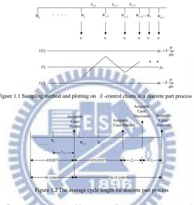
For discrete part Weibull process, samples of size are drawn in every h hours j

of production, and the sample means are plotted on the x _{control charts which has an}

control limit at . The sampling method and plotting on x-control charts in

a discrete part process is shown in Figure 1.1. And the average cycle length for discrete part process is illustrated in Figure 1.2.

12 W_j Wj1 Wj2 Wj3 Wk Wk1 n UCL CL LCL 0 k n    0 k n    0 

‧ ‧

1  j h hj2 hj3 ... n n n n n 0 W ．．．．

Figure 1.1 Sampling method and plotting on x-control charts in a discrete part process

j W 1  j W Wj2 . . . . AVGICT AVGOOCT Z1 Z2

In control Out of control Assignable Cause Detected Assignable Cause Discovered Assignable Cause Removed Assignable Cause Occures 1  j 

Figure 1.2 The average cycle length for discrete part process

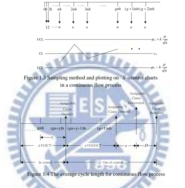
For continuous flow exponential process, sampling scheme is to take one sample

from the process at each sampling time and then combine analytical results into a

subgroup. The sample means are plotted on x-control charts which has an control limit

at . The sampling method and plotting on x-control charts in a continuous

flow process is shown in Figure 1.3. And the average cycle length for continuous flow process is illustrated in Figure 1.4.

13 _nh UCL CL LCL 0 k n    0 k n    0 

‧ ‧

n n n 0 …... 2nh 3nh …... …... gnh n n n (g1)nh(g2)nh …... h 2h 12 …...

Figure 1.3 Sampling method and plotting on x-control charts

in a continuous flow process

. . . .

In control Out of control

Assignable Cause Detected Assignable Cause Discovered Assignable Cause Removed Assignable AVGICT AVGOOCT gnh (gn+j)h (gn+j+1)h (g+1)nh i  e D Cause Occures

Figure 1.4 The average cycle length for continuous flow process

We assume that there are s possible assignable causes and the occurrence time of any one assignable cause follows Weibull or Exponential distribution. The occurrences of

s assignable causes are independent to each other. Once assignable cause A_i occurs, it continues to affect the process until it is detected by control chart, and during this period it is allowed for the second occurrence of an assignable cause following the first occurrence. The process at any time is either in control or out of control which resulted in

a  i shift amount in the process mean by the occurrence of the ith assignable cause

i

14

non-increasing functions of the _i’s), they are J-shaped, rectangular and half-bell shaped.

These distributions would cover the distribution most likely to meet in reality. Therefore,

three prior distributions of _i are considered. There are negative-exponential

((1 2) exp(i 2)), uniform and half-normal (

2

(1 2 ) exp( (0.5 )  i 2)). Finally, to

simplify the analysis, we assume that the joint effect of the two assignable causes is

always to produce a shift of  in the process mean regardless of what two

assignable causes occur jointly. Consequently, there is no need to consider the prior distribution of the second assignable causes.

A production cycle begins when a new system is installed and ends when the process is brought back to an in-control state after a system failure is detected and repaired. The objective is to find optimal values for sample size, control limit coefficient, and sample interval such that the expected loss-cost per unit time is minimized.

1.5 Scope of Dissertation

The main purposes of this dissertation are to analyze: (i) the economic design of x

-control charts for discrete part Weibull process with multiple assignable causes; and (ii)

the economic design of x-control charts for continuous flow exponential process with

multiple assignable causes. This dissertation is organized by four chapters as follows: Chapter 1 is an introduction, which shows the background of the control charts,

earlier studies on the economic design of x-control charts. The inspection interval

principle relevant to this study is also presented.

In Chapter 2, we study the economic design of x-control charts for discrete part

Weibull process with multiple assignable causes. The expected cycle length and the total expected cost per cycle are derived by using the inspection intervals principle. Next, the expected loss-cost function is constructed by the ratio of the expected cycle length and

15

the total expected loss-cost per cycle. We determine the optimal design parameters ( n,

k, and h1 ) of the model to minimize the expected loss-cost function. In addition,

comparison is also investigated. Finally, we provide numerical results among the optimal design parameters, the minimal expected loss-cost function and the specific value of design parameters.

In Chapter 3, we consider another the economic design of x-control charts for

continuous flow exponential process with multiple assignable causes. The occurrence time of any one assignable cause follows Exponential distribution. For such type of process, we construct the expected loss-cost function based on the the expected cycle length and the total expected loss-cost per cycle. In addition, the optimal design

parameters ( n, k , and h ) of the model can be analytically determined to minimize

the expected loss-cost function. Finally, sensitivity analysis is investigated, and a numerical result is also provided.

Chapter 4 presents some conclusions based on results of the investigation, and recommendations for the future investigations.

16

Chapter 2

Economic Design of

x

-Control Charts for Discrete Part

Weibull Process with Multiple Assignable Causes

In this chapter, we study the economic design of x-control charts for discrete part

Weibull process with multiple assignable causes. A modified version of Chen and Yang’s

model [8] for the x-control charts is proposed to deal with situations involving the

multiple assignable causes. In Chen and Yang’s model, it is assumed that once an assignable cause occurs, no further assignable causes will occur. To ascertain the effect of this assumption, a study is conducted in this chapter that allows for the second occurrence of an assignable cause following the first occurrence. For manufacturers, the economic objective of production is very important and has to be optimized. An

economic approach is developed for the design of x-control charts. Therefore, we adopt

Duncan’s multiple causes model [15], Banerjee and Rahim’s sampling scheme [3], and Chen and Yang’s cost structure [8] to develop a modified model. A modified model is the

economic design of x-control charts for discrete part process with Weibull in control

times which subjects to a multiplicity of assignable causes.

This chapter is organized as follows: In Section 2.1, we give some basic definition and assumptions of the model under study and give some notations. Section 2.2 presents the formulation of the expected cycle length by using the inspection interval principle. In Section 2.3, we develop the total expected loss-cost per cycle. And the expected loss-cost function is constructed. In Section 2.4, we determine the optimal design parameters. Finally, in Section 2.5, a numerical example will be presented to compare the optimal results between the modified model and Chen and Yang’s model.

17

(1) The occurrence time of the ith assignable cause (denoted as Ai, i1, 2, , s)

that the process remains in the in-control state follows a Weibull distribution and the probability density function is given by

1

( ) it , 0, 1, 0, 1, 2, , .

i i i

f t t e  t    i s (2.1)

The hazard rate is 1

( )

i i

r t  t , where i, i1, 2, , s, is a scale parameter

and  is a shape parameter.

(2) The process is normally distributed and characterized by an in-control state ₀,

because of the occurrence of an assignable cause A which occurs at random, _i

resulting in a shift in the mean from ₀ to either



₀

 

_i or



₀

 

_i . Where

0

 ,  , and _i are, respectively, the process mean, the process standard deviation,

and shift parameter.

(3) The occurrence of the ith assignable cause A does not affect the process _i

variability, that is, the process mean and the process variability are independent. (4) The shift in the process mean is instantaneous.

(5) The time to sample and to draw control point is negligible and production ceases during the searches and repair.

(6) Define pij (i1, 2, , , s j1, 2, ) as a conditional probability that the ith

assignable cause A will occur during the sampling interval_i hj1, given that the

cause A_i is not occur at time Wj, that is

1 ( ) ( 1) 1 ( ) ( ) 1 exp( ( ) ) ( ) W j W W i j i j i W j ij i W i j i W j f t dt _{e e} p h e f t dt              _  



  



. (2.2)

From the above Equation (2.2), the pij is a function of i, h1, and  only. Let

ij i

p  p , for i1, 2, , , s j1, 2, .

18 1 0 0 1 1 1 1 1 (1 ) 0 0 ( ) ( ) 1 1 ( ) ( ) (1 ) ( ) (1 ) (1 ) , W j i ij ij j i W j j j W j j i i i i i pi W j j j i q t W f t dt t f t dt j h p p  h p p A       _    _                 











occur during the sampling interval hj1. The q can be obtained from Equation ij

(2.2). 1 ( ) (1 ) , for 1, 2, , , 1, 2, W j j ij i ij ij W j q 



 f t dt  p p i s j . (2.3)

(8) Let ij be the expected duration of the in-control period within the sampling

interval hj1, given that the ith assignable cause A occurred during this sampling i

interval, that is 1 ( ) ( ) W j j i W j ij ij t W f t dt q    



. (2.4)

Thus, the expected in-control time i during any one sampling interval in which

the transition is from an in-control state to an out-of-control state is given by

(2.5) where ( ) ₀( 1)1 l x _l A  l  x 





  , for x 1, and ( )y is gamma function, y1.

In this chapter, the following notations shall be used in the formulation of the loss-cost function.

n － the sample size (decision variable)

j

h － the length of the jth sampling interval, where j1, 2, , h0 0

(decision variable)

k － the control limit coefficient (decision variable)

0

Z － the expected search time associated with the false alarm

1

19

2.2 Formulation of the expected cycle length

We assume that there are s possible assignable causes and the occurrence time of

any one assignable cause follows Weibull distribution. The occurrences of s assignable

causes are independent to each other. After being disturbed by an assignable cause A , _i

the process will be affected by any other assignable causes. In the other hand, if the first assignable cause continues undetected, the second assignable cause (possibly a repetition

has been detected

2 i

Z － the expected time to repair process once the cause A has been i

discovered, where i1, 2, , s

2

Z  － the expected time to repair process once the joint assignable cause has

been discovered

0

D － the quality cost per unit time while producing in control

Y － the cost per false alarm while producing in control

1i

D － the quality cost per unit time while producing out of control owing to the

occurrence of the ith assignable cause A , where _i i1, 2, , s

1

D － the quality cost per unit time while producing out of control owing to the

occurrence of the joint assignable cause

i

w － the cost to locate and repair the ith assignable cause A , where _i

1, 2, ,

i s

w － the cost to locate and repair the joint assignable cause

a － the fixed sample cost

20

of the first) is assumed to occur at random in a later intervals.

The occurrence time of the second assignable cause after the taking of the first

sample being distributed Weibull with the mean 1

(1)  (1 1 ) and the probability

density function of occurrence will be 1

( ) t , 1, 0, 0

f t   t e     t . The

process is assumed to be in one of the three states. It is (1) in a state of in control or (2) it

has been disturbed by the occurrence of the ith assignable cause Ai which produces a

shift of  i in the process mean or (3) it has been disturbed by the occurrence of the

second assignable cause following the first, the joint effect of which in every case is

arbitrarily assumed to produce a shift of  in the process mean. The expected cycle

length consists of three states, which can be derived as follows: (1) State 1:

The probability at time

t

in control is

0 1 2 1 2 ( ) ( , , , ) ( ) ( ) ( ) t s s P T  t P A t A t A  t P A  t P A   t P A  t e  , (2.6) where 0 1 s i i

  and then the probability density function of occurrence of multiple

assignable causes will be 1

0( ) 0 exp( 0 ), 1, 0 0, 0

f t   t  t    t , thus the

average time in control is 1

0

(1 )  (1 1 ) .

Therefore, the process is in an in-control state and the expected time that the

assignable cause will occur is 1

0

(1 )  (1 1 ) .

(2) State 2:

The process has been disturbed by the occurrence of the first assignable cause and

produces a shift of  i in the process mean. When the process is in State 2, it is

assumed that no further disturbance occurs until after the first sample is taken. The process can be classified into two situations.

21

Consider Situation 1 for Figure 2.1. Situation 1 is the period that the second

assignable cause will not to be occurring until assignable cause A is detected. _i

Let i be the probability of type II error, that is, the probability that control point

falls inside control limits after the occurrence of the first assignable cause. Thus,

( ) ( )

i k i n k i n

        , where  ( ) is the cumulative distribution of the standard normal.

Define E T( )1 as the expected time that is from the occurrence of the first

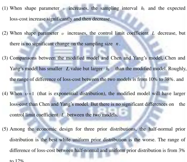
assignable cause A to the cause _i A has detected, discovered, and removed, which can _i

be expressed as: (2.7) where h1 i ie        , 1 1 ih i

p  e , and i is given by Equation (2.5).





















1 1 '₁ 1 1 2 1 0 1 1 2 1 0 1 (1 ) ( ) ( ) 1 1 (1 ) ( ) (1 ) (1 ) (1 ) (1 )(1 ) 1 k W j h i j k j i i i i W j k j j k i i i j k j i i i k j i i i i i i Pi i i i i i i E T f t dt W W e Z Z p p W W Z Z P P P h A P P P                                  _{ }   _  _          _       _                    

 



1 _(i) i 1 2i, h A_   Z Z i A i  …… Z1 Z2i 1 h e  nh …… 1  j W 1 h e  Detected 2  j W Wj3 Discovered ) 1 ( i i  i i  1 ( ) E T j W ……

Figure 2.1. The process of Situation 1 for State 2 in a discrete part process.

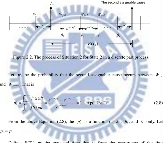
22 Situation 2:

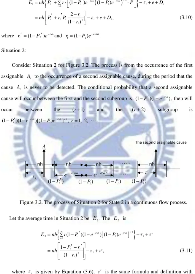
Consider Situation 2 for Figure 2.2. Situation 2 is the period that from the occurrence of the first assignable cause to the occurrence of the second assignable cause

and during this period that the assignable cause A_i is never to be detected.

Let p2 be the probability that the second assignable cause occurs between Wj i

and Wj ( 1)i _{. That is} 2 1 2 1 2 1 1 1 ( ) 1 exp( ) ( ) W j Wj Wj W j W j W j f t dt _{e e} p h e f t dt                _{  }   _        





. (2.8)

From the above Equation (2.8), the p2 is a function of , h1, and  only. Let

2

p p.

Define E T( 2) as the expected time that is from the occurrence of the first

assignable cause A_i to the occurrence of the second assignable cause, which can be

expressed as: i  …… 1 h e  nh ……

Figure 2.2. The process of Situation 2 for State 2 in a discrete part process.

1  j W Wj2 Wj3 i  i  i  i  2 ( ) E T j W ……

The second assignable cause

1 h e  nh i A

23 (2.9) where h1 i ie   _   , 1 1 ih i p  e  , and (1 )1 (1 1 ) h p1 (1 p A) (1p)             .

Let AVGOOCT2i be the expected time to detect the first assignable cause, once the

ith assignable cause A has occurred. To summarize the Situation 1 and 2, we obtain _i

the AVGOOCT2i as following:

2i ( )1 1 2i ( )2

AVGOOCT E T Z Z E T . (2.10) Then the average length of runs in State 2 resulting from the initial assignable cause

i A _{, respectively, is.} 1 2 [ 2] ( ) ( ) E State E T E T . (2.11) (3) State 3:

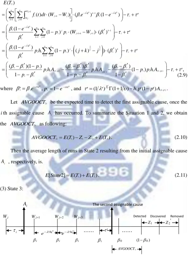
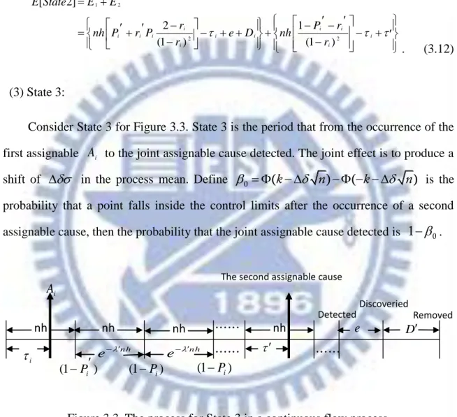
Consider State 3 for Figure 2.3. State 3 is the period that from the occurrence of the





2 1 '_{1 1} '₁ 1 0 '₁ 1 1 1 1 0 '₁ 1 1 1 ( ) ( ) ( ) ( ) (1 ) (1 ) (1 ) ( ) ( ) (1 ) (1 ) ( ) ) W j h k h i j k j i i i W j k j h i j k i i j k j i i k j i h i j i i i E T f t dt W W e e e p p W W e p h p j k j                _{  }      _                     _{ }   _  _        _   _     _            

 



1 0 1 (1 ) 1 _{( )} 1 (1 ) ( ) ( )(1 ) ( ) ( ) (1 ) , 1 1 1 k i i k j i i i i i i i i i pi i _i i i pi i i i i i i p p h A p h A p p h A p p            _{ }                         _  _{ }   _   _    _            



 2 Z 3i AVGOOCT  h1 e  nh  h1 e  nh i   i  i i i 0 (10) i A 1  j W Wj2 Wj3

The second assignable cause causecause

……

Figure 2.3. The process for State 3 in a discrete part process.

1 Z Detected Discovered …… j W Removed

24

second assignable cause to the joint assignable cause detected. The joint effect is

assumed to produce a shift of  in the process mean. Let the probability of detecting

a shift of  be 0, 0    (k  n)    ( k  n).

Define

P

2i

(

i



1, 2,

, )

s

as the probability that the second assignable cause will

occur after the occurrence of the first assignable cause, which can be expressed as:

(2.12) where h1 i ie   _   .

Let AVGOOCT3i be the expected time of detecting the joint assignable cause. The

expression for the AVGOOCT3i is given by

(2.13)

Let E State( 3) as the average length of runs in State 3 resulting from the initial

assignable cause A is i





3 1 2 2

( 3) i i

E State  AVGOOCT  Z Z P . (2.14)

Let r1 be the expected number of samples taken in the “in-control” period. Then

the r1 can be expressed as:

1 ₀ 1 0 0 0 1 1 0 1 ( ) (1 ) ( ) W j j W j j j p r j f t dt j p p p  _     











   , (2.15) 1 1 1 1 2 1 0 1 1 1 0 1 ( ) ( ) (1 ) (1 ) ( ) (1 ) (1 ) , 1 1 W j h k h i i i i W j k j h k j i i i i k j h i i i i i P f t dt e e e p p e                    _                  _{ }                 

 







   



3 1 1 0 0 2 1 0 0 0 1 (1 ) 1 (0) 2 0 0 ( ) 1 (1 ) (1 ) . 1 1 i W j k j k j i W j k j p i AVGOOCT f t dt W W P p p p h A p h A P p p       _     _            _ _    _  _           _{ }   _{ }       

 

25

where 0 1

0 1

h

p  e .

The expected number of false alarms per cycle before the process goes out of

control will be  times the expected number of samples taken in the “in-control” period,

where  2 1



 ( )k



. The expected number of false alarms per cycle will thus be r1.

Therefore, the expected time of finding false alarms will be Z0( )r1 .

The occurrence rate of the assignable cause A in total s assignable causes is _i

assumed to be  i 0. The average length of runs in some “out-of-control” state that

result from the initial assignable cause A is the sum of the average run length in State 2 _i

plus the average run length in State 3. The overall mean time for a cycle will thus be





0 1 0 1 0 0 1 1 1 ( ) ( ) (1 ) ( 2) ( 3) s i i p E T E State E State Z p            



   . (2.16)

2.3. Formulation of the expected loss-cost per cycle

Based upon the above derivation of the expected cycle length, the ingredients of

expected loss-cost per cycle E C( ) are as follows:

(1) The expected quality cost per cycle of in-control state is

1 0 0 1 1 ( ) (1 ) D       . (2.17)

(2) The expected cost per cycle of out-of-control state is



1 2 1 3



1 0 s i i i i i D AVGOOCT D AVGOOCT      



. (2.18)

(3) The expected cost per cycle to locate and repair the assignable cause is



2 2



1 0 (1 ) s i i i i i P w P w       



. (2.19)

(4) The expected sampling cost per cycle is

1 2 3 1 0 ( ) ( ) s i i i i a bn  r r r    



   . (2.20)

26

(5) The expected cost per cycle of finding false alarms is

1

( )

Y  r . (2.21)

(6) Let r2 i be the expected number of samples taken in State 2 when the assignable

cause A_i has occurred. Let r3i be the expected number of samples taken in State 3.

The r2 i and r3i are expressed as Equation (2.22) and (2.23).

(2.22)

where i iexp( h1 )



     .

(2.23)

To summarize, we obtain the expected loss-cost per cycle as following:

(2.24) 1 1 3 2 0 0 1 0 1 2 0 0 1 2 0 ( ) ( ) (1 ) (1 ) ( ) 1 . 1 W j k i i i W j k j k i k i r P k f t dt P k P        _            _ _{ }  _        _   _     

 







1 0 0 1 2 1 3 2 2 1 0 1 2 3 1 0 0 0 1 1 ( ) ( ) (1 ) (1 ) ( ) ( ) 1 ( ). s i i i i i i i i s i i i i E C D D AVGOOCT D AVGOOCT P w P w a bn r r r p Y p                          _     _      





1 1 2 1 1 0 1 1 1 1 1 0 1 2 2 2 ( ) ( exp( )) (1 ) ( ) ( exp( )) (1 exp( )) 1 (1 exp( )) (1 ) (1 ) 1 , (1 ) W j k i i i i W j k j W j k i i i W j k j i i i i i i r k f t dt h k f t dt h h h                     _      _        _ _{ }    _         _ _{ }      _                   

 

 

27

Finally, the expected loss-cost function E A( ) is constructed by the E T( ) and

) (C

E . Our objective is to find the optimal design parameters n , h and k to ₁

minimize the E A( )E T( ) E C( ) based on the given values of time, cost and shift

parameters.

2.4. Determination of optimal design parameters

The parameters involving in the expected loss-cost function can be classified into

cost parameters (Y D; 0; D1i; D w1; i; w ; ;  a b), time parameters (Z ; 0 Z1; Z ; 2i Z2), shift

parameters (i;  ), Weibull distribution parameters ( i; ) and design parameters

(n ; ; h1 L). A numerical example is used to illustrate the performance of the model. We

assume that Y$2000 per false alarm, D0 $210 per unit time, D1$4000 per unit

time, a$20 per sampled, b$20 per unit sampled, w$1000 per cycle, Z01.25

hours, Z11.25 hours, Z22 hours, 0.02,   2 and they remain the same for

the different assignable causes. D1i, wi, Z2i, and i are taken to be a function of i

and the rules of selection are as follows:

(1) The i is a non-increasing function of the i for all i. When the cause A occurs, _i

0

 will shift to   0 i . D1i is proportional to the resulting increase in the

percent of product outside specification (0i    1 (3 i)   ( 3 i) 1   (3 i),

for i1, 2, , s ). From the repeated production experiment, the more the

occurrence of shift, the lower values of wi and Z2 i are.

(2) Assume the process exists seven assignable causes (A ii, 1, 2, , 7), those causes

will produce 1 , 1.5 , 1.8 , 2 , 2.2 , 2.5 , and 3 shift amount, respectively,

the occurrence of any one assignable cause are random and independent.

(3) Z2 i, D1i, and wi are functions of i. Assume that i 2, D1i, wi, and Z2 i are

28

(4) Owing to obtain i, we assume that 1 1 1 80

s

ii Di  D

     .

Let PDi denoted the prior distribution of i (11, 21.5, 31.8, , 73).

In this section, the negative-exponential, uniform, and half- normal distribution are

considered for PDi. Let the prior distribution of 4=2 be PD4. We set up the values of

the time parameters and the cost parameters for 4=2 as “base case”, and in one set, i

are chosen as proportional to PDi. According to the discussion of above (1), (2), (3),

and (4) rules, we assume that wi (PD PDi 4) 1000 , Z2i (PD PDi 4) 2 ,

1i ( 0i 04) 4000

D     since 4=2 and i (PD PDi 1)1. The values of wi, Z2 i,

and i for different prior distributions and the values of D1i for different i are

displayed in Table 2.1.

Table 2.1

The set of cost and probability parameters.a

i A i 0i i PD 1i D 2i Z wi 3 ( 10 ) i  _  i NE Uni HNi NEi Uni HNi NEi Uni HNi NEi Uni HNi 1 1 0.0228 0.303 0.143 0.352 575 3.29 3 2 2.90 9 1647 1000 1454 4.566 2.294 4.220 2 1.5 0.0668 0.236 0.143 0.301 1684 2.56 5 2 2.48 8 1283 1000 1244 3.557 2.294 3.608 3 1.8 0.1151 0.203 0.143 0.266 2901 1.10 3 2 2.19 8 1103 1000 1099 3.059 2.294 3.190 4 2 0.1587 0.184 0.143 0.242 4000 2 2 2 1000 1000 1000 2.772 2.294 2.901 5 2.2 0.2119 0.166 0.143 0.218 5341 1.80 4 2 1.80 2 902 1000 901 2.502 2.294 2.612 6 2.5 0.3085 0.143 0.143 0.183 7776 1.55 4 2 1.51 2 777 1000 756 2.155 2.294 2.194 7 3 0.5 0.112 0.143 0.130 12602 1.21 7 2 1.07 4 609 1000 537 1.689 2.294 1.557 a i

NE , Negative-exponential; Uni, Uniform; HNi, Half-normal.

2.5. Comparison with Chen and Yang’s model

Chen and Yang [8] assumed once assignable cause A occurs, it continues to affect i

the process until it is detected by the control chart, and during this period it is undisturbed by the occurrence of other assignable causes. Owing to compare the model, the computer program developed in this work is available from us. We used search technique which is

29

k . Table 2.2 compares the effect that variation in Weibull parameter values has on the

economic design of x-control charts. With the same data, for several sets of , cost

comparisons between the modified model and Chen and Yang’s model for different sets of Weibull shape parameter.

Table 2.2 indicates the following general conclusions:

(1) When shape parameter  increases, the sampling interval h1 and the expected

loss-cost increase significantly and then decrease.

(2) When shape parameter  increases, the control limit coefficient L decrease, but

there is no significant change on the sampling size n .

(3) Comparisons between the modified model and Chen and Yang’s model, Chen and

Yang’s model has smaller Lvalue but larger h1 than the modified model. Roughly,

the range of difference of loss-cost between the two models is from 10% to 38%. and

(4) When 1 (that is exponential distribution), the modified model will have larger

loss-cost than Chen and Yang’s model. But there is no significant differences on the

control limit coefficient L between the two models.

(5) Among the economic design for three prior distributions, the half-normal prior distribution is the best while uniform prior distribution is the worse. The range of difference of loss-cost between half-normal and uniform prior distribution is from 3% to 12%.