具頻域等化機制之單載波空時區塊碼之盲蔽式多通道判別---以非多餘傳送前置編碼為基礎的研究

行政院國家科學委員會補助專題研究計畫

■ 成 果 報 告

□期中進度報告

具頻域等化機制之單載波空時區塊碼之盲蔽式多通道判別：

以非多餘傳送前置編碼為基礎的研究

計畫類別：■ 個別型計畫 □ 整合型計畫

計畫編號：NSC 95－2221－E－009－047－MY2

執行期間： 96 年 8 月 1 日至 97 年 7 月 31 日

計畫主持人：李大嵩 教授

共同主持人：吳卓諭 助理教授

計畫參與人員：林光敏、黃崇榮、李思漢、宋志晟

成果報告類型(依經費核定清單規定繳交)：□精簡報告 ■完整報告

本成果報告包括以下應繳交之附件：

□赴國外出差或研習心得報告一份

□赴大陸地區出差或研習心得報告一份

■出席國際學術會議心得報告及發表之論文各一份

□國際合作研究計畫國外研究報告書一份

處理方式：除產學合作研究計畫、提升產業技術及人才培育研究計畫、

列管計畫及下列情形者外，得立即公開查詢

□涉及專利或其他智慧財產權，□一年□二年後可公開查詢

執行單位：

中 華 民 國 97 年 10 月 29 日

摘要

本計畫基於非冗長對角先期編碼和獨立同分佈（i.i.d.）訊源的假設，提出以 單載波頻域等化器為基礎的空時區塊碼系統的盲蔽式通道估測法。此方法開發了 共軛交叉相關介於兩個時間區塊信號的先期編碼所產生的線性信號結構和循環 行列式的通道矩陣特性，並且在通道雜訊為循環高斯而接收機資料統計可以完整 的得到時可以產生精確解。 此通道估測的公式化建立在重組共軛交叉相關矩陣的線性方程式集合以及 通道脈衝響應，使之成為一個具有區塊循環循環區塊（block-circulant with circulant-block (BCCB)）的特殊結構。這樣允許了一個簡單的僅視先期編碼參數 而定的可辨識條件，也提供了一個自然而有效的最佳先期編碼器的設計架構來改 善當不完全資料估測發生時的解答正確性。 我們從明確和統計的觀點考慮兩種資料不匹配的模型，並且提出相關的設計 準則。最佳化的問題以利用 BCCB 系統矩陣的特性公式化並加以分析求解。所 提出的最佳化先期編碼器目的在於有明確誤差擾動時解的強健度最佳化和當資 料不匹配以白雜訊模型化時的均方誤差最小化。配對的誤差機率分析用來探討等 化器的性能，而數值分析的例子便展示了提出方法的性能。 關鍵詞：盲蔽式通道估測， 具有循環區塊的區塊循環矩陣，循環矩陣，多輸入 單輸出，非冗長先期編碼器，單載波頻域等化器，空時區塊碼，傳送多樣性 I

Abstract

Relying on non-redundant diagonal precoding and i.i.d. source assumption, this

paper proposes a blind channel estimation scheme for single-carrier

frequency-domain equalization based space-time block coded systems. The proposed

method exploits the precoding-induced linear signal structure in the conjugate

cross-correlation between the two temporal block received signals as well as the

circulant channel matrix property, and can yield exact solutions whenever the channel

noise is circularly Gaussian and the receive data statistic is perfectly obtained. The

channel estimation formulation builds on rearranging the set of linear equations

relating the entries of conjugate cross-correlation matrix and products of channel

impulse responses into one with a distinctive block-circulant with circulant-block

(BCCB) structure. This allows a simple identifiability condition depending on

precoder parameters alone, and also provides a natural yet effective optimal precoder

design framework for improving solution accuracy when imperfect data estimation

occurs. We consider two models of data mismatch, from both deterministic and

statistical points of view, and propose the associated design criteria. The optimization

problems are formulated to take advantage of the BCCB system matrix property and

are solved analytically. The proposed optimal precoder aims to optimize solution

robustness against deterministic error perturbation and also minimize the mean square

error when the data mismatch is modeled as a white noise. Pair-wise error probability

analysis is conducted for investigating the equalization performance. Numerical

examples are used to illustrate the performance of the proposed method.

Keywords: Blind channel estimation, block-circulant matrix with circulant blocks

(BCCB), circulant matrix, multiple input single output (MISO), nonredundant

precoders, single-carrier frequency-domain equalization, space–time block code

(STBC), transmit diversity.

Contents

Abstract I

Chapter 1 Introduction 1

Chapter 2 System Model and Basic Assumptions 6

Chapter 3 Blind Channel Estimation 9

Chapter 4 Identifiability and Product Unknowns Computation 17

Chapter 5 Optimal Precoder Design 21

Chapter 6 Equalization Aspect 31

Chapter 7 Simulation Results 33

Chapter 8 Conclusions 45

Appendix 47

References 55

Chapter 1

Introduction

A. Overview

Space-time block code (STBC) is a widely-known transmit diversity technique for

combating channel fading in modern wireless communications [22]. Most of the

existing proposals are devised for the flat- fading channel environment, e.g., the

Alamouti’s scheme [1] and the related generalization by Tarokh et. al [34], among

others. When the propagation channels are subject to frequency-selective fading, one

popular STBC technique is via time-reversal block-wise encoding, either combined

with OFDM mechanism [27], [40], or resorting to time-domain equalizer [26], for

removing the channel distortion. The multi-carrier related solutions, although

simplifying receiver implementations, would incur high peak-to-average power ratio

(PAPR) and is sensitive to carrier frequency offset. The scheme with time-domain

equalization, on the other hand, can provide additional multipath diversity at the

expense of decoding complexity. To avoid the drawbacks of the multi-carrier strategy

and to also maintain low receiver complexity, an alternative single-carrier

frequency-domain equalization (FDE) based STBC was proposed in [2]. The

aforementioned STBC’s capable of mitigating dispersive channels can be cast into a

general code formulation [39]; comparisons pf the achievable performances and

implementation costs can be found in [3].

known at the receiver to coherently combine the multiple temporal received signals

for decodinga. Since STBC potentially entails low spectral efficiency and training based channel estimation further consumes bandwidth resource, blind approaches

then become appealing candidate solutions. There has been extensive literature on

blind multi-input multi-output (MIMO) channel estimation [14], [16]. However, only

a few studies are tailored for STBC systems, typically through a multi-input

single-output (MISO) channel link. Under flat-fading assumption, several schemes

were put forth for orthogonal STBC [4], [7], [32], and for a general linear code family

[33]. For time-reversal STBC over frequency-selective channels, the work [5] focused

on codes with time-domain equalization [26]. Through linear symbol precoding, blind

schemes for OFDM-based STBC were shown in [27] and [40]. The method [27]

resorts to zero-padding for removing inter-block interference, and is applicable only

for constant-modulus sources and channel pairs without common zeros; the one in

[40], instead, uses cyclic prefix (CP) as guard interval and leverages redundant

precoding to relieve the source and channel-zero constraints imposed in [27]. For

FDE-STBC, training based channel estimation is recently considered in [11]. It is

known that single-carrier FDE systems fall within the class of precoded OFDM, with

FFT matrix as precoder [25]. In view of this fact, the method in [40] for OFDM

scenario also provides an immediate blind solution for FDE-STBC: one just chooses

FFT precoding matrix to convert the multi-carrier transmission into a single-carrier

scheme and then inserts certain redundancy into the symbol streams to facilitate

channel identification. The price to be paid for this approach, however, would be the

a

Differential STBC does not require channel information for decoding but incurs a 3-dB penalty in

loss in the effective data rate.

B. Paper Contributions

This paper proposes a blind channel estimation scheme for FDE-STBC systems in a

two transmit antennas and single receive antenna environment. The proposed

approach relies on non-redundant diagonal precoding (hence preserving the baud

rate), assumes i.i.d. source statistics (irrespective of constellation modulus), and does

not impose constraints on sub-channel zero locations. It exploits the

precoding-induced linear signal structure in the time-domain conjugate

cross-correlation between the two temporal receive branches, as well as the circulant

channel matrix property after CP is discarded. Specifically, we show that the set of

linear equations relating the entries of conjugate cross-correlation matrix and products

of channel impulse responses can be rearranged into one with a block-circulant with

circulant-block (BCCB) structure. The products of channel taps are first obtained by

solving this linear equation set; the channel pair is then simultaneously identified, up

to a 2 2 complex matrix ambiguity, as the dominant left singular vectors of an × associated rank-two matrix. A similar “bilinear” estimation strategy has also been

adopted in [13], [21], [24], [37]. In our formulation, a natural sufficient condition for

unique channel recovery is the non-singularity of certain BCCB matrix with precoder

coefficients as its entries. Channel identifiability is thus free from any priori

assumptions on sub-channel characteristics, and is shown to be fulfilled by almost all

choices of precoders. As long as the channel noise is circularly Gaussian and the

received data statistic is perfectly obtained, the resultant channel estimate is exact. In

the presence of finite-sample estimation error, the proposed channel estimation

robustness. We consider two models of data mismatch, one as an unknown

deterministic perturbation while the other statistically as a white noise, and propose

the associated optimal precoder design criteria, aiming for minimizing the worst-case

solution sensitivity to perturbation and mean-square errors, respectively. Both

optimization problems are further formulated to take advantage of the BCCB system

matrix property and are then analytically solved; the resultant solutions are shown to

be the same two-level form precoder. Pair-wise error probability (PEP) analysis is

conducted to investigate the equalization performance of the proposed optimal

solution and characterize the associated design trade-off. It is noted that blind channel

estimation via non-redundant diagonal precoding has been considered in the single

channel case [31], [10], [24], [37]; the related generalizations to MIMO single- and

multi-carrier spatial multiplexing systems can be found in [8] and [9]. The rest of this

paper is organized as follows. Section II briefly describes the system model and the

underlying assumptions. Section III presents the proposed method; the associated key

features are investigated in Section IV. Section V addresses the optimal precoder

design against imperfect data estimation. Section VI examines the equalization

performance through PEP analysis. Section VII contains the simulation results.

Finally, Section VIII is the conclusion.

Notation List: Let Rm n× and Cm n× be respectively the sets of m× real and n complex matrices. Denote by ( )⋅ , T ()⋅ , and ()* ⋅ , respectively the transpose, H complex conjugate, and Hermitian operations. The symbols I and _m 0 denote the _m

m m× identity and zero matrices; 0_{m n×} is the m× zero matrix. The notation n ⊗ stands for the Kronecker product [19, p-242]. For _X∈Cm n×

with x_j ∈Cm being the jth column, define vec( ) : [X = xT₁ xT T_n] ∈C . For mn x∈C , let m

{ }

diag x be the m m× diagonal matrix with the elements of x on the main diagonal. The notation Ey stands for the expected value of the random variable y ,

and j:= − . We denote by 1 F∈CN N× the FFT matrix with the kl-th entry

[ ] ( 1)( 1) , : 1/ k l k l N ω − − − = ⋅

F , where ω: exp( 2 / )= j π N , 1≤k l, ≤N . We denote

Chapter 2

System Model and Basic Assumptions

We consider the discrete-time baseband model of an FDE-STBC system [2] over

frequency-selective channels as shown in Figure 1. Let s and _k s_{k +1} be two

N-dimensional symbol blocks to be transmitted. Priori to the STBC encoder, each

symbol block is precoded by an N×N diagonal matrix

[

]

{

}

:=diag p(0) p N( −1)T P , (2.1) with p n( )∈ , to obtain R l = l x Ps , for l =k k, + , 1 (2.2)

which are then spatially and temporally coded according to [2] for transmit diversity

as well as for mitigating the multipath channel distortion. For 1≤ ≤ , let ( )i 2 h n _i be the impulse response of the channel between the ithtransmit antenna and the receive antenna. In terms of block signals, the input-output relations in time-domain

are described as [2]

1 2 1

k k + k+ + k

y = G x G x v , (2.3)

1 2

1 1 1

k+ = k+ − k + k+

y G x G x v , (2.4)

where, for l =k k, + , 1 y and _l v are the received signal (upon CP removal) and _l noise, x_l is the time-reversed and element-wise conjugated version associated with

l x , that is, * ( ) (( ) ) l n = l −n N x x , 0≤ ≤n N − , 1 (2.5)

and G_i ∈CN N× is circulant withb

C

: (0) ( ) 0 0T N

i = ⎡⎢_⎣hi h Li ⎤⎥_⎦ ∈

g , (2.6)

as the first column, 1≤ ≤ . Since i 2 G is circulant, we have _i G_i =F D FH _i , where i D is diagonal with ( 1) 0 ( ) L m n i _mm i n h n ω− − = ⎡ ⎤ ₌ ⎣ ⎦D

∑

, 1≤m ≤N . Let us define : l = l

Y Fy , X_l :=Fx , and _l V_l := Fv , for _l l =k k, +1 . Then the

frequency-domain representation associated with (2.3) and (2.4) can be expressed in a

compact vector-matrix form as [2]

1 2 * * * * 1 2 1 1 1 : k k k k k+ + k+ = ⎡ ⎤ ⎡ ⎤_{⎡ ⎤} ⎡ ⎤ ⎢ ⎥ ₌ ⎢ ⎥⎢ ⎥₊⎢ ⎥ ⎢ ⎥ ⎢₋ ⎥⎢ ⎥ ⎢ ⎥ ⎢ ⎥ ⎢ ⎥⎢_⎣ ⎥_⎦ ⎢ ⎥ ⎣ ⎦ ⎣ ⎦ ⎣ ⎦ D Y D D _X V X Y D D V ; (2.7)

through space-time matched filtering using the effective channel matrix D we get

* * 1 1 1 k N k k H H k k+ N + k+ ⎡ ⎤ ⎡ ⎤ _{⎢ ⎥}⎡ ⎤ ⎡ ⎤ ⎢ ⎥ _{= ⎢ ⎥}⎢ ⎥₊ ⎢ ⎥ ⎢ ⎥ _{⎢ ⎥}⎢ ⎥ ⎢ ⎥ ⎢ ⎥ ⎢_⎣ ⎥_⎦ ⎢ ⎥ ⎣ ⎦ ⎣ ⎦ ⎣ ⎦ Y D 0 X V D D X Y 0 D V , (2.8) b

Without loss of generality we may take L as a common channel order, or simply an associated upper

where D:=D DH_{1 1}+D D₂H ₂ ∈RN N× is diagonal with 2 2 1_ii 2 _ii ii ⎡ ⎤ ₌ ⎡ ⎤ ₊ ⎡ ⎤ ⎢ ⎥ ⎣ ⎦ ⎣ ⎦ ⎣ ⎦D D D ,

1≤ ≤i N: this asserts that two-fold transmit diversity is achieved in the frequency domain. To recover the source signals, per-tone frequency-domain equalizer [2], [15]

can be designed based on (2.8), as long as a channel estimate is available at the

receiver. Based on the time-domain signal model (2.3) and (2.4), this paper proposes a

blind channel estimation scheme by using the second-order statistics of the received

signal and discusses an optimal design of the precoder ( )p n for improving channel estimation accuracy. The following assumptions are made in the sequel.

a) The source sequence ( )s n is independently identically distributed (i.i.d.) with zero mean and Es k s l( ) ( )* =δ(k − , where ()l) δ⋅ is the Kronecker delta function.

b) The noise ( )v n is white circular Gaussian with zero mean, variance σ_v2, and is independent of the source sequence ( )s n .

Chapter 3

Blind Channel Estimation

To introduce the proposed method, we first assume that all the signal statistics can

be perfectly obtained; the case with imperfect data estimation will be treated later. To

obtain the channel matrix D , one may focus on direct estimation of the N tones of

the channel frequency response. Since the block length N could be large, this strategy

would involve considerable computational efforts. Hence, we propose to instead

estimate the time-domain channel impulse response ( )h n , for 0_i ≤ ≤ and n L 1≤ ≤ ; the gains of the associated frequency tones can then be obtained by using i 2 FFT operations.

A. Identification Equations

The proposed approach exploits the imbedded linear signal structure in the

time-domain conjugate cross-correlation matrix of the two received signals y and _k

1

k +

y as well as the circulant property of the channel matrix G . To proceed, let us _i

first define the matrix

R 1 0 0 0 1 : 0 1 0 1 0 N N× ⎡ ⎤ ⎢ ⎥ ⎢ ⎥ ⎢ ⎥ =⎢ ⎥∈ ⎢ ⎥ ⎢ ⎥ ⎢ ⎥ ⎢ ⎥ ⎣ ⎦ Γ . (3.1)

Then, from (2.5), it is easy to see

* k = k x Γ and x * 1 1 k+ = k+ x Γx . (3.2)

With (2.2) and (3.2), the signal models (2.3) and (2.4) then become y = G Ps_{k 1 k} +G Ps_{2 k+1}+v , _k (3.3) and * * 1 2 1 1 1 k+ = k+ − k + k+ y G PsΓ G PsΓ v . (3.4)

From (3.3), (3.4), and by assumptions a) and b), it is easy to check

{

}

2 2 2 1 1 2 1 2 1 1 1 1 1 (1) : T T T T T T k k k k k k k k E ₊ Γ Γ E ₊ E _{+ +} E ₊ = = − + + + y R y y G P G G P G G P s v G P s v v v . (3.5)

Since the noise ( )v n is circular, we have Ev v_{k k}T₊₁ =0 . Also, we assume that both _N the real and imaginary components of the noise process are independent of those of

the source sequence ( )s n : this thus implies Es v_{k k}T₊₁ =Es_k+1vT_k+1 =0 . Under _N these conditions, the noise contributions to the conjugate cross-correlation matrix

(1) y

R in (3.5) become a zero matrix, leading to

2 2

2 1 1 2

(1)₌ T ₋ T

y

R G P GΓ G P GΓ . (3.6) For a given R_y(1), the matrix equation (3.6) defines a set of N scalar equations 2 nonlinear in the unknowns h_i(0), , h L_i( ) 1, ≤ ≤ , but is linear with respect to i 2

product channel coefficients h k h l , _i( ) ( )_i 1≤i i, ≤ . As a result, in lieu of directly 2 solving for h_i(0), , h L , we propose to exploit the imbedded linear structure in _i( )

(1) y

R for channel estimation. This will be done by further taking into account the

circulant property of the channel matrices G ’s. _i

R 1 ( 1) 1 ( 1) 1 1 : N N N N N × − _× − − × ⎡ ⎤ ⎢ ⎥ = _{⎢ ⎥} ∈ ⎢ ⎥ ⎣ ⎦ 0 J I 0 . (3.7)

Since G is circulant, it can be expressed in terms of its first column (cf. (2.6)) as _i

2 1 N N i i i i i − − ⎡ ⎤ = ⎢_⎣ ⎥_⎦ G g Jg J g J g , 1≤ ≤ . i 2 (3.8)

By definitions of P and Γ (see (2.1) and (3.1)) and from (3.8), it follows

(

) (

)

( )

2 2 1 2 2 2 1 2 1 1 2 2 2 1 1 2 2 2 2 1 1 1 2 1 0 (0) (1) ( 1) ( ) . T T T N T N n N N n T T n p p p N − − − p n − = = ⋅ ⎡ ⎤ ⎡ ⎤ =_⎢⎣ − _{⎥ ⎢⎦ ⎣}⋅ _⎥⎦ = = =

∑

G P G G P G g Jg J g g J g Jg J g g J G P G Γ Γ Γ (3.9) Similarly, we have

( )

1 2 2 1 2 1 2 0 ( ) . N _{N n} T n T T n p n − ₋ = =

_∑

G P GΓ J g g J (3.10)

Combining (3.9) and (3.10), R_y(1) in (3.6) becomes

( )

1 2 0 (1) N ( ) n T N n n p n − ₋ = =

∑

y R J G J , (3.11) wherec 1 2 1 1 2 2 ₁ 2 : T T T N N T × ⎡ ⎤ ⎢ ⎥ ⎡ ⎤ = − = _{⎢ ⎥}⋅_{⎢ ⎥}∈ ⎣ _{⎦ ⎢− ⎥} ⎣ ⎦ g G g g g g g g g C . (3.12)

With g given in (2.6), the matrix G is seen to contain the product channel _i impulse responses of the form h k h l₂( ) ( )₁ −h k h l₁( ) ( )₂ , ,0≤k l ≤ , which are to be L determined from (3.11). Toward a tractable procedure for computing G , we observe

c

We assume that the two channel impulse response vectors are linearly independent, for otherwise G

is identically a zero matrix; this assumption holds whenever the environment is with sufficiently rich

that R_y(1) in (3.11) is a weighted sum of N matrices of the form J G Jn

( )

T N n− , in which the unknown G are pre, and post, multiplied by the known matrices Jn and

( )

JT N n− . Based on this structural property, we can further rearrange (3.11) into a standard linear equation form. This is done via the next lemma.

Lemma 3.1 [19, p-255]: The matrix equation 1 K k k k = =

∑

A XB C can be equivalently expressed as 1 ( ) ( ) K T k k k vec vec = ⎡ ⎤ ⎢ ⊗ ⎥ = ⎢ ⎥ ⎣

∑

B A ⎦ X C . …

Based on Lemma 3.1, we can immediately rewrite (3.11) as

1 2 0 ( ) ( ) ( (1)) N N n n n p n vec vec − − = ⎡ ⎤ ⎢ ⊗ ⎥ = ⎢ ⎥ ⎣

∑

J J ⎦ G Ry . (3.13)

By definitions of the Kronecker product and J in (3.7), equation (3.13) turns out to

be 2 2 2 2 2 1 2 1 2 2 3 2 2 2 2 2 3 2 2 2 2 2 2 1 2 (0) (1) ( 2) ( 1) ( 1) (0) ( 3) ( 2) (2) (3) (0) (1) (1) (2) ( 1) (0) : N N N N N N N N N N p p p N p N p N p p N p N p p p p p p p N p − − − − − − ⎡ _{− −} ⎤ ⎢ ⎥ ⎢ ⎥ ⎢ − − − ⎥ ⎢ ⎥ ⎢ ⎥ ⎢ ⎥ ⎢ ⎥ ⎢ ⎥ ⎢ ⎥ ⎢ ⎥ − ⎢ ⎥ ⎢ ⎥ ⎣ ⎦ = I J J J J I J J J J I J J J J I Q ( ) ( (1)) vec G =vec R_y (3.14)

The N2×N2 real-valued matrix Q defined in (3.14), which is characterized by the N circulant matrices

{

p(0)2I_N, , p(1)2J , p N( −1)2JN−1

}

on the top row block, is block circulant with circulant blocks (BCCB) [12, p-184]. Equation (3.14)

B. Identification of Channel Impulse Response

Assume that vec G , and hence the matrix G , can be uniquely recovered from

( )

the linear equation (3.14); the uniqueness condition and the computational issue will

be investigated in the next section. We then collect the product unknowns

2( ) ( )1 1( ) ( )2

h k h l −h k h l , 0≤k l, ≤ , to form the following (L L+ ×1) (L+ matrix 1)

, , 0 : _{k l} k l L ≤ ≤ ⎡ ⎤ = ⎢_⎣ ⎥_⎦ H H , where H_{k l,} =h k h l₂( ) ( )₁ −h k h l₁( ) ( )₂ . (3.15) Observe that the matrix H is of rank two, and can be factorized as

1 2 1 1 2 1 2 2 0 1 1 0 T T T T ⎡ ⎤ ⎡ _{− ⎤ ⎢ ⎥} ⎡ ⎤ ⎢ ⎥ = − = _{⎢⎣ ⎥ ⎢⎦ ⎥⎢ ⎥} ⎢ ⎥ ⎢ ⎥ ⎣ _{⎦ ⎣ ⎦} h H h h h h h h h , (3.16) where C 1 : (0) (1) ( )T L i hi hi h Li + ⎡ ⎤ =_{⎢⎣ ⎥⎦} ∈ h , 1≤ ≤ , i 2 (3.17)

is the desired channel impulse response vectors. Based on (3.16), the channels can

thus be identified, up to a 2× complex matrix of the form 2

a b c d ⎡ ⎤ ⎢ ⎥ = ⎢ ⎥ ⎢ ⎥ ⎣ ⎦ U , with ad−bc = , 1 (3.18)

by computing the two dominant left singular vectors associated with H ; the inherent

matrix ambiguity must satisfy (3.18) since, for any vector pair of the form

1 2 ⎡ ⎤ = ⎢_⎣ ⎥_⎦ h h h U with U∈C2 2× , we have 2 1 1 2 0 1 1 0 T T T ⎡ − ⎤ ⎢ ⎥ _{= −} ⎢ ⎥ ⎢ ⎥ ⎣ ⎦ h h h h h h (3.19)

approach for blind channel estimation is also adopted in [13], [21], [24], [37].

C. On Ambiguity Removal

The matrix ambiguity (3.18) can be resolved through insertion of additional pilot

symbols. To see this, let ⎡_⎢⎣h₁ h₂⎤_⎥⎦ be a dominant left singular vector pair associated

with the rank-two matrix H defined in (3.15). Then we have

1 2 1 2

⎡ ⎤ ₌ ⎡ ⎤

⎢ ⎥ ⎢ ⎥

⎣h h ⎦ ⎣h h U⎦ , with U∈C2 2× fulfilling (3.18); this implies

1 1 1 2 1 2 1 2 1 2 a b d b c a c d − − ⎡ ⎤ ⎡ − ⎤ ⎡ ⎤ ₌ ⎡ ⎤ ₌ ⎡ ⎤⎢ ⎥ ₌⎡ ⎤⎢ ⎥ ⎢ ⎥ ⎢ ⎥ ⎢ ⎥⎢ ⎥ ⎢ ⎥⎢− ⎥ ⎣ ⎦ ⎣ ⎦ ⎣ ⎦_{⎢ ⎥} ⎣ _{⎦ ⎢⎣ ⎥⎦} ⎣ ⎦ h h h h U h h h h . (3.20)

Since both G and ₁ G are circulant, the first output branch (2.3), at some ₂ k =k₀, can be alternatively expressed as

0 0 1 0 1 2 0

k k + k + + k

y = C g C g v , (3.21)

where g _i (i=1 2), is the zero-padded channel impulse response as in (2.6), and N N

l

×

∈

C C is circulant with the precoded symbol vector x as the first column, _l

0, 0 1 l =k k + . Let us write 1 ( 1) T T i = ⎢⎡_⎣ i ×N L− − ⎤⎥_⎦ g h 0 , 1≤ ≤ , i 2 (3.22)

where h is the desired channel impulse response vector defined in (3.17). With _i (3.22), equation (3.21) is then reduced to

0 0 1 0 1 2 0

k k + k + + k

y = C h C h v , (3.23) where C_l ∈CN× +(L 1) contains the first L +1 columns of C . With (3.20), we can _l

write (3.23) in terms of the scalar ambiguities as

(

)

(

)

0 0 0 0 0 0 0 0 0 1 2 1 1 2 1 2 1 1 1 2 : . k k k k T k k k k k d c b a d c b a + + + = = − + − + + ⎡ ⎤ ⎡ ⎤ = _⎢ − − _{⎥ ⎢⎣ ⎥⎦} + ⎣ ⎦ T y C h h C h h v C h C h C h C h v (3.24)

It is noted that, subject to the constraint ad−bc = , there are only three 1 independent unknowns in (3.24). One can just solve for, say (b c d , from (3.24) and , , ) then determine a via the nonlinear equation a =(1+bc d)/ ; this, however, would be more prone to error propagation. Hence we propose to instead compute (a b c d , , , ) all at once from (3.24). Toward this end, pilot symbols should be appropriately

inserted to produce at least four training components in

0

k

y . We observe that each

column of T in (3.24) is a linear combination of L +1 circularly shifted symbol vector x for some _l l ∈{ ,k k_{0 0} +1}. The cyclicity structural constraint implies at least L +4 pilot symbols are needed in both x . One plausible placement, in _l particular, is to insert four (and L , respectively) consecutive pilots at the head (and

tail) of x , _l l =k k₀, ₀ + ; in this way, the first four components in 1

0

k

y , denoted by

t

y , then act as training data and the scalar unknowns are estimated via

1 T t t d c b a − ⎡ _{⎤ =} ⎢ ⎥ ⎣ ⎦ T y , (3.25)

where T_t ∈C4 4× contains the first four rows of T .Hence, even though the proposed blind method reduces the number of unknown channel parameters from

2L +2 to three, no less than 2L +8 pilot symbols are nonetheless required for ambiguity removal. This is due to the non-redundant precoding based channel

estimation formulation as well as the circulant signal structure (the proposed channel

Chapter 4

Identifiability and Product Unknowns

Computation

This section first specifies the channel identifiability condition, and then introduces

two methods for computing the product channel coefficients. The presented results

also lay the foundation for further investigating the optimal precoder design problem.

A. Channel Identifiability

From the previous discussions, it is easy to see that the channel can be identified if

( )

vec G is uniquely determined from (3.14): this is true if the matrix Q is

nonsingular. By exploiting the BCCB property of Q , the following theorem

explicitly shows the associated eigenvalues, and in turn specifies the condition for Q

to be nonsingular. Roughly speaking, if we define the vector

R

= 2 2 − 2 ∈

: [ (0)_{p p}(1) _{p N}( 1) ]T N

p , (4.1)

then the N eigenvalues of Q are completely determined by the N eigenvalues 2 associated with the N×N circulant matrix with p as the first row (the proof of T theorem is given in Appendix A).

Theorem 4.1: Let F be the N×N FFT matrix; also, associated with the vector p

in (4.1) we define the polynomial

2 2 1 2 ( 1)

( ) :_{z = p}(0) _+p(1) _z− _{+ +p N}( ₋1)_z−N−

Then the N eigenvalues of the matrix Q defined in (3.14) are given by the N 2 replicas of the N -tuple

{

p(1) ( ), , pω , p(ωN−1)

}

.

…

Theorem 4.1 shows that channel identifiability is guaranteed whenever p(ω ≠n) 0 for all 0≤ ≤n N − ; this condition is quite mild and can hold for almost all 1 choices of ( )p n . We should note that the significance of Theorem 4.1 is far above just characterizing a sufficient condition for unique channel recovery. It moreover

specifies the eigenvalues associated with the matrix Q : this result will be exploited

for selecting ( )p n to improve the reliability of channel estimate against the finite-sample estimation error (see Section V).

B. Computation of

vec G

( )

A crucial step for implementing the proposed channel estimation scheme is the

computation of the product channel coefficient vector vec G based on (3.14). In

( )

what follows we propose two methods for fulfilling this task.

i) Direct Matrix Inversion: An immediate approach to solving (3.14) is through

direct matrix inversion so that

( )

1

(

₍₁₎

)

vec G =Q− vec R_y . (4.3)

Observe from (3.14) that Q is BCCB and is characterized by the particular set of

circulant matrices

{

p(0)2I_N, , p(1)2J , p N( −1)2JN−1

}

. This appealing structure allows for a potentially low-complexity implementation via FFT operations. In

Appendix B we derive a simple closed-form expression of Q based on which this −1 figure of merit is justified.

ii) Solution via Zero Entry Removal in (3.14): It is noted from (2.6) that, for

1≤ ≤i 2 , the vector g contains _i L+1 channel impulse response ( )h n , _i

0≤ ≤ , followed by n L N − − trailing zeros. As a result, the L 1 2 2

N

N × matrix

2 1 1 2

(= T − T)

G g g g g , and hence the associated vectorized representation vec G , has ( ) actually (L +1)2 nonzero product unknowns. By removing the zero entries in

( )

vec G , and the corresponding indexed columns of the matrix Q , equation (3.14)

can be simplified to a set of N scalar equations in 2 (L +1)2 unknowns. Indeed, with g defined in (3.22), we have _i

( 1) ( 1) 1 ( 1) ( 1) H i i L N L H i i N L N L L + × − − − − − − × + ⎡ ⎤ ⎢ ⎥ = ⎢ ⎥ ⎢ ⎥ ⎣ ⎦ h h 0 g g 0 0 , 1≤i i, ≤ 2 (4.4) and hence 2 1 1 2 T T = − = G g g g g ( 1) ( 1) 1 ( 1) ( 1) L N L N L N L L + × − − − − − − × + ⎡ ⎤ ⎢ ⎥ ⎢ ⎥ ⎢ ⎥ ⎣ ⎦ H 0 0 0 , (4.5)

where H is defined in (3.15). Based on (4.5) and by definition of the vec ⋅ () operation, equation (3.14) can be shown (after some direct manipulations) to be

reduced into

(

)

1 1 2 ( ) ( (1)) : L+ ⊗ vec =vec = y QJ I J H R Q (4.6) in which R 2 ( 1) _{( 1)} 1 ( 1) ( 1) N L _{N N L} N N L N L + _{× +} − − × + ⎡ ⎤ ⎢ ⎥ =_{⎢ ⎥} ∈ ⎢ ⎥ ⎣ ⎦ I J 0 and R 1 _{( 1)} 2 ( 1) ( 1) : L N L N L L + _{× +} − − × + ⎡ ⎤ ⎢ ⎥ = _{⎢ ⎥} ∈ ⎢ ⎥ ⎣ ⎦ I J 0 .

(4.7)

The matrix Q∈RN2× +(L 1)2 in (4.7) is obtained by deleting N2 −(L+1)2 columns from Q . It is thus of full column rank whenever Q is nonsingular and, if so, the

product channel coefficients can be computed via

(

)

1

( ) T T ( (1))

vec H = Q Q − Q vec R_y . (4.8)

Compared with the direct matrix inversion method (4.3), the solution (4.8) can yield

better estimation accuracy at the expense of computational complexity (see Appendix

B for complexity evaluation). Based on (4.3) and (4.8), the selection of precoder

( )

Chapter 4

Optimal Precoder Design

If the conjugate cross-correlation matrix R_y(1) is perfectly obtained, both solutions (4.3) and (4.8) are exact. In practice, however, only a finite number of data

samples can be used for estimating R_y(1); equations (3.14) and (4.6) should be accordingly modified as ˆ ( (1)) ( ) vec Ry =QvecG +w , (5.1) and ˆ ( (1)) ( ) vec R_y =Qvec H +w , (5.2)

where ˆ (1)R_y is an estimate of R_y(1) and w accounts for the data mismatch due

to finite-sample estimation. Given the error-corrupted ˆ (1)R_y , it is impossible to recover the actual product channel coefficients. Instead, with (5.1) and (5.2), the

estimated solutions are respectively

1 1

ˆ _ˆ

( ) : ( (1)) ( )

vec G =Q− vec Ry =vec G +Q w − (5.3) and

( )

ˆ :

vec H =

(

Q QT

)

−1QTvec(Rˆ_y(1))_=vec( )_{H +}

(

_{Q Q}T

)

−1_{Q w}T

. (5.4)

In what follows, we consider two different modeling schemes of w , and propose the

A. Minimal Worst-Case Sensitivity to Error Perturbation

We will first treat w as an unknown “deterministic” perturbation since the

statistical property of the data estimation error is in general difficult to characterize.

From this standpoint, typical solution robustness measures for (5.3) and (5.4) are the

condition numbers of the matrices Q and Q , respectively (see, e.g., [18] and [23]).

Small κ Q and ( )( ) κ Q , in particular, are known to ensure small worst-case sensitivity of the error-perturbed solution to data mismatch [18, p-338]. Since both Q

and Q depend entirely on ( )p n , a natural approach to improving the channel estimation accuracy is to choose ( )p n so that both ( )κ Q and ( )κ Q are kept as small as possible. This type of optimization problem would seem formidable to tackle

since the condition number of a matrix is in general a highly nonlinear function in the

entries. Toward a tractable design formulation, we note the crucial fact: since Q

contains a subset of columns of Q (see (4.6)), it follows [23, p-27]

( ) ( )

κ Q ≤κ Q . (5.5)

Inequality (5.5) suggests that, to jointly improve the accuracy of solutions (5.3) and

(5.4), it is plausible to just minimize ( )κ Q because a small ( )κ Q will also guarantee ( )κ Q to be small. Such a design strategy, on the one hand, can bypass direct minimization of ( )κ Q which would appear rather intractable. More importantly, it will allow us to exploit the eigenvalue characteristics of the BCCB

matrix Q (in Theorem 4.1) to analytically derive a solution, as is shown below.

constraints 1 2 0 ( ) N n p n N − = =

∑

, (5.6a) and

min ( )p n 2 ≥ for some δ 0< <δ 1. (5.6b)

The constraint (5.6a) normalizes the average transmit power within one block to unity,

and the constraint (5.6b) imposes a minimal threshold on the floor power. In the

context of single channel blind identification based on

modulation-induced-cyclostatonarity, the two constraints have been used in [10], [24],

and [37] for precoder design against the channel noise effect.

To derive the optimal solution, we shall first specify ( )κ Q in terms of the eigenvales of the matrix Q . Since Q is BCCB, it can be factorized as

( )

(

H H

)

= ⊗ ⊗

Q F F Λ F F for some diagonal Λ [12, p-181]. This then implies that

Q is a normal matrix [18, p-100], as can be seen by

( )

(

)

( )

(

)

( )

(

)

( )

(

)

; = H H H H H H H H H H H H H = ⊗ ⊗ ⊗ ⊗ = ⊗ ⊗ = ⊗ ⊗ = Q Q F F F F F F F F I F F F F F F F F QQ Λ Λ Λ Λ ΛΛ (5.7)

in deriving (5.7), we have used the identity (A⊗B C)( ⊗D)=AC⊗BD [19, p-244]. As Q is normal, it is known that [18, p-340]

( )

( )

1

( )

κ Q =ρ Q ρ Q− , (5.8)

in which (ρ M): max | |:=

{

λ λ's are eigenvalues of the matrix M . Equation (5.8)

}

links the condition number of Q with the extreme magnitudes of the associated

eigenvalues which, according to Theorem 4.1, are exactly the maximum and

minimum among the N elements

{

| (1) |p , |p( ) |ω , , |p(ωN−1) |

}

, where ( )pz is the polynomial defined in (4.2). More precisely, we have

max ( ) ( ) min ( ) k k ω κ ω = p Q p , for 0≤ ≤k N − . 1 (5.9)

To find the minimal ( )κ Q based on (5.9), we shall further characterize ( )p ωk ’s under the two constraints in (5.6). With (5.6a), it is easy to see from (4.2) that, for

0 k = , 1 0 2 0 ( ) (1) N ( ) n p n N ω − = = =

∑

= p p . (5.10)

The following lemma provides an upper bound on p( )ωk for 1≤ ≤k N − ; the 1 result is crucial for deriving the minimal ( )κ Q (the proof of lemma is shown in Appendix C).

Lemma 5.1: For any ( )p n satisfying (5.6a) and (5.6b), we have

( )ωk ≤N(1−δ)

p for all 1≤ ≤k N − . 1 (5.11)

…

With (5.9), (5.10), and (5.11), the minimal achievable ( )κ Q , and the corresponding optimal ( )p n , are shown in the following theorem.

Theorem 5.2: Under the constraints (5.6a) and (5.6b), the minimal condition number associated with the matrix Q is given by

min 1 ( ) 1 κ δ = − Q , (5.12)

which is attained by the following two-level solution: for a fixed but arbitrary

0≤m ≤N − , 1

2

( ) ( 1)

p m =N − N − δ, and p n( )2 = for nδ ≠m. (5.13)

[Proof]: We claim that i) ( )κ Q ≥1/(1−δ) for any ( )p n satisfying (5.6a) and (5.6b), and ii) equality is attained by the solution (5.13); the theorem thus follows. To

show claim i), it is noted from (5.9) and (5.10) that

0

max ( ) ( )

( )

min ( ) min ( ) min ( )

k k k k N ω ω κ ω ω ω = p ≥ p = Q p p p . (5.14)

Also, (5.10) and (5.11) imply

min ( )p ωk ≤N(1−δ), i.e., 1 1

(1 )

min ( )_{p ω}k ≥ _{N −δ} . (5.15)

Claim i) then follows immediately from (5.14) and (5.15). To prove claim ii), it is

noted that solution (5.13) yields, for any k ≠ , 0

{

}

1 2 0 ( )k N ( ) kn ( 1) km kn n n m p n N N ω − ω− δ ω− δ ω− = ≠ =

_∑

= − − +

_∑

p

{

}

{

}

, 1 0 (1 ) km N kn (1 ) km n N δ ω− δ − ω− N δ ω− = = − +

_∑

= − (5.16)

where the last equality follows since

1 0 0 N kn n ω − − = =

∑

for any k ≠ . Equations (5.10) 0 and (5.16) show that, with solution (5.13), we have max ( )p ωk = p( )ω0 =N and

max ( ) ₁ ( ) (1 ) 1 min ( ) k k N N ω κ δ δ ω = = = − − p Q p . (5.17)

The proof is thus completed. …

Theorem 5.2 shows that

min( )

κ Q depends entirely on the minimal power threshold δ , irrespective of the dimension of Q (and hence the symbol block length N ). A

small δ , in particular, is seen to yield small

min( )

κ Q and thus improves the channel

estimation accuracy.

B. Minimization of Mean Square Error

In this subsection, we alternatively formulate w as a zero-mean white noise

vector with covariance matrix σ I , and resort to the well-known minimum mean _w2 square error principle, see, e.g., [6], for constructing a solution. Although a theoretical

justification of such statistical data error assumption is difficult to establish, our

simulation study does confirm this tendency.

Since w is white, the mean square errors incurred by solutions (5.3) and (5.4) are,

respectively,

(

)

2 ₁ 2 ˆ ( ) ( ) _w H E vec −vec =σ Tr⎡_⎢ − ⎤_⎥ ⎣ ⎦ G G Q Q (5.18) and

(

)

2 ₂ 1 ˆ ( ) ( ) _w H E vec −vec =σ Tr⎡_⎢ − ⎤_⎥ ⎣ ⎦ H H Q Q (5.19)

be chosen to jointly minimize Tr⎡_⎢

(

H

)

−1⎤_⎥ ⎣ Q Q ⎦ and

(

)

1 H Tr⎡_⎢ − ⎤_⎥ ⎣ Q Q ⎦, (5.20)

subject to the constraints (5.6a) and (5.6b). Minimization of this type of cost functions

has been considered in least-squares based channel estimation, e.g., [6] and [22, chap.

9], among others. The reported solution approach therein is via the following

inequality: since both Q Q and H Q Q are positive definite, it follows H

(

)

1 1 , H H i i i Tr⎡_⎢ − ⎤_⎥ ≥ ⎡_⎢⎣ ⎤_⎥⎦− ⎣ Q Q ⎦

∑

Q Q and

(

)

1 1 , H H i i i Tr⎡_⎢ − ⎤_⎥≥ ⎡_⎢⎣ ⎤_⎥⎦− ⎣ Q Q ⎦

∑

Q Q , (5.21)

and equalities in (5.21) hold whenever Q Q and H Q Q , respectively, are diagonal H [28, p-1041]. If the power normalization equation (5.6a) is the only design concern, it

is easy to check that the impulse sequence

2

( )

p m =N , and p n = for n( )2 0 ≠m, (5.22) where 0≤m≤N − is fixed but arbitrary, simultaneously diagonalizes 1 Q Q H and Q Q , and is thus the jointly minimizer. However, given the additional threshold H power requirement (5.6b), one cannot rely on this principle for finding a solution

since, subject to the BCCB structure of Q and p n > , it is impossible to choose ( )2 0 ( )

p n to render both Q Q and H Q Q diagonal. In what follows we propose an H

alternative strategy to address the considered optimization problem. Our approach is

grounded on a key fact shown in the next lemma, which directly establishes an

inequality relation analogue to (5.5) regarding the two cost functions in (5.20) (the

proof is given in Appendix D).

Lemma 5.3: Let M be a square nonsingular matrix, and M be constructed from

(

_H

)

1

(

_H

)

1 Tr⎡_⎢ − ⎤_⎥ ≤Tr⎡_⎢ − ⎤_⎥ ⎣ M M ⎦ ⎣ M M ⎦. (5.23) … Lemma 5.3 asserts Tr⎡_⎢

(

H

)

−1⎤_⎥ ⎣ Q Q ⎦ is upper bounded by

(

)

1 H Tr⎡_⎢ − ⎤_⎥ ⎣ Q Q ⎦. This thus suggests a suboptimal, but would be more simple and efficient, way of precoder

design: we can simply choose ( )p n to minimize Tr⎡_⎢

(

H

)

−1⎤_⎥

⎣ Q Q ⎦ , since

(

_H

)

1

Tr⎡_⎢ − ⎤_⎥

⎣ Q Q ⎦ would in turn be kept small. The main advantage of the proposed design formulation, as expected, is that we can directly take profit of the BCCB

property of Q to derive a closed-form solution. Indeed, since Tr⎡_⎢

(

H

)

−1⎤_⎥

⎣ Q Q ⎦ is the

sum of the eigenvalues associated with

(

Q QH

)

−1 which, according to Theorem 4.1, are exactly the N replicas of the N -tuple

{

| ( ) |ωn −2

}

_{0 n N 1}

≤ ≤ − p , we have

(

)

1 1 2 0| ( ) | N H k k N Tr ω − − = ⎡ _{⎤ =} ⎢ ⎥ ⎣ Q Q ⎦

∑

p . (5.24) Equation (5.24) rewrites Tr⎡_⎢

(

H

)

−1⎤_⎥ ⎣ Q Q ⎦ in terms of ( ) n ω

p ’s; we can then further

exploit equation (5.10) and Lemma 5.1 to construct an optimal solution, as is shown

in the next theorem.

Theorem 5.4: The optimal ( )p n minimizing Tr⎡_⎢

(

H

)

−1⎤_⎥

⎣ Q Q ⎦, subject to constraints (5.6a) and (5.6b), is the two-level solution (5.13). The resultant minimal mean square

error is 2 2 2 min ( 1) (1 ) w w N MSE N N σ σ δ − = + − . (5.25)

[Proof]: From (5.10), we have

(

)

1 1 1 1 2 2 2 2 0 1 1 1 | ( ) | | (1) | | ( ) | | ( ) | N N N H k k k k k k N N N N Tr N ω ω ω − − − − = = = ⎡ _{⎤ = = + = +} ⎢ ⎥ ⎣ Q Q ⎦

∑

p p

∑

p

∑

p . (5.26)

From Lemma 5.1, it follows

2 2 2

1 1

(1 )

( )ωk ≥N −δ

p , 1≤ ≤k N − , 1 (5.27)

with equality attained by the two-level sequence (5.13) (this is easily seen from

(5.16)). From (5.26) and (5.27), the minimal Tr⎡_⎢

(

H

)

−1⎤_⎥

⎣ Q Q ⎦ is thus

(

)

1 1 2 2 min ₁ 1 1 1 1 (1 ) (1 ) N H k N Tr N N δ N N δ − − = − ⎡ ⎤ _{= + = +} ⎢ ⎥ ⎣ Q Q ⎦

∑

− − . (5.28)

Equation (5.25) follows directly from (5.28), and this thus proves the theorem. …

Recall that the impulse sequence (5.22) is optimal with regard to the power

normalization constraint (5.6a). When an additional power threshold is imposed, it

turns out that the best choice is the “impulse-like” two-level solution (5.13). With

(5.25), the resultant MSE_min is seen to decrease whenever δ is decreased. Hence, a small δ not only limits solution sensitivity to deterministic error perturbation (as we

have shown in the previous subsection), but also improves the estimation accuracy

against white data estimation error. From the equalization point of view, it is however

undesirable to keep δ unlimitedly small; this will be further discussed in the next

section.

Remarks:

objective functions ( )κ Q and Tr⎡_⎢

(

H

)

−1⎤_⎥

⎣ Q Q ⎦ are quite different in nature, the respective minimizing solutions, under constraints (5.6a) and (5.6b), are the same

the two-level form choice (5.13); this is due to the BCCB property of the matrix

Q .

(b) The two-level solution (5.13) minimizes both ( )κ Q and Tr⎡_⎢

(

H

)

−1⎤_⎥

⎣ Q Q ⎦, but its

optimality with respect to ( )κ Q and Tr⎡_⎢

(

H

)

−1⎤_⎥

⎣ Q Q ⎦ appears intractable to verify. Our simulation results seem to indicate that it is indeed the minimizing solution.

(c) Since κ( )Q ≤κ( )Q and Tr_⎢⎡

(

H

)

−1⎤_⎥ ≤Tr⎡_⎢

(

H

)

−1⎤_⎥

⎣ Q Q ⎦ ⎣ Q Q ⎦, solution (5.4) can yield better estimation accuracy than (5.3); numerical simulations (see Simulation 2)

also evidence this tendency.

(d) The optimal solution (5.13) does not depend on the index m at which the peak

power occurs: any 0≤m ≤N − allows for an utmost mitigation for data 1 estimation error. However, since the trailing components in each symbol block

will be duplicated as CP, the peak power in (5.13) should not be located within the

corresponding index region so as to conserve the power resource.

(e) In the study of single channel blind identification via modulation-induced-

cyclostationarity, the two-level sequence (5.13) is shown to be optimal for

mitigating the channel noise effect for the serial transmission case [10], [24], and

Chapter 6

Equalization Aspect

Toward symbol recovery in FDE-STBC systems, one commonly used approach is via frequency-domain per-tone equalization [2], [15] based on (2.8), commonly in conjunction with linear ZF or MMSE criterion. In this section we resort to ZF-PEP analysis [35] for investigating the equalization performance regarding the optimal solution (5.13).

To proceed, based on (2.2), we shall first expand the linearly combined frequency-domain signal model (2.8) into

* * * 1 1 1 1 1 , 1 , 1 _, : : : : k N k k N N k k H H H k N k k N k N k k k k k Φ _{k k} + + + + + + + ⎡ ⎤ ⎡ ⎤ ⎡ ⎤ _{⎢ ⎥}⎡ ⎤ ⎡ ⎤ _{⎢ ⎥}⎡ _{⎤ ⎡ ⎤} ⎡ ⎤ ⎢ ⎥ _{= ⎢ ⎥}⎢ ⎥ ₊ ⎢ ⎥ _{= ⎢ ⎥}⎢ _{⎥ ⎢ ⎥ +} ⎢ ⎥ ⎢ ⎥ _{⎢ ⎥}⎢ ⎥ ⎢ ⎥ _{⎢ ⎥}⎢ _{⎥ ⎢ ⎥} ⎢ ⎥ ⎢ ⎥ ⎢_⎣ ⎥_⎦ ⎢ ⎥ ⎢_⎣ ⎥_⎦ ⎣ ⎦ ⎢ ⎥ ⎣ ⎦ ⎣ ⎦ ⎣ ⎦ ⎣ ⎦ ₌ ⎣ ⎦ = = = Y D 0 X V D 0 FP 0 s V D D _s D 0 FP X Y 0 D V 0 D V s Z _V 1 + (6.1) or by dropping the block index k and k +1 for notational simplicity,

Φ

= +

Z s V . (6.2)

The PEP measures the probability that a symbol block s is transmitted but another ≠

s s is detected. Given the channel realizations h and ₁ h , the conditional PEP is ₂

by definition given by

1 2 1 2

Pr⎡_⎣s→s h h| , ⎤_⎦ =Pr_⎣⎡ s− < −s s s h h , | , _⎦⎤ (6.3)

where ˆs is the estimate of s under the ZF metric and, from (6.2), is given by

1 1

ˆ :_{s =}Φ−_{Z= +s} Φ− _{V .}

(6.4)

By following the procedures as in [35] and define d =: s−s , the conditional PEP in (6.3) can be upper bounded by

1 1 ₁ 2 2 2 2 1 1 2 2 1 1 2 0 Pr | , 4 _v 4 _v N ( ) F F F n Q d σ Q d σ p n − − ₋ − − − − = ⎛ _{⎛ ⎞} ⎞ ⎛ ⎛ ⎞ ⎞⎟ ⎜ ⎜ ⎛ ⎞ ⎟ ⎟⎟ ⎜ ⎟ ⎜ ⎜ ⎟ ⎟ ⎡ → ⎤≤ ⎜⎜ ⎜⎜ ⎟ ⎟⎟= ⎜⎜ ⎜⎜ ⎜ ⎟⎟ ⎟⎟ ⎟⎟ ⎣ ⎦ ⎜⎜⎝ ⎜⎝ ⎟⎠ ⎟⎠⎟ ⎝⎜⎜⎜ ⎜⎜⎝ ⎝⎜⎜

∑

⎠⎟ ⎟⎟⎠ ⎟⎟⎟⎟⎠ s s h h P D D , (6.5) where Q ⋅ denotes the Gaussian tail, and the equality in (6.5) follows directly from ( ) (2.1). For a given channel pair, and hence D , the upper bound in (6.5) is minimized

if the quantity 1 2 0 ( ) N n p n − − =

∑

attains the minimum. Since, by the Cauchy’s inequality,

(

_p(0)−2 _{+ +p N( −1)}−2

)(

_p(0)2 _{+ +p N( −1)}2

)

_≥(_{1+ +1})2 _=N2 , (6.6) and 1 2 0 ( ) N n p n N − = =

∑

(cf. (5.6a)), we have

(

p(0)−2 + +p N( −1)−2

)

≥N , with equality holds if and only if ( )p n = for 01 ≤ ≤n N − . This shows the equal 1 power scheme is optimal from an equalization point of view. Any form of precoding induced power variation, therefore, will incur a loss in the decision performance. The precoder (5.13), however, turns out to be the worst-case choice, as can be seen from the following theorem (see Appendix E for a proof).

Theorem 6.1: For all ( )p n satisfying (5.6a) and (5.6b), the solution (5.13)

maximizes the quantity 1 2 0 ( ) N n p n − − =

∑

, leading to 1 2 0 1 1 max ( ) ( 1) N n N p n N N δ δ − − = − = + − −

∑

. (6.7) … Based on (6.7), simple manipulation shows the maximum value, when viewed as a function of δ , will increase as δ is decreased. As a result, a small δ , although improving channel estimation accuracy, will enlarge the PEP upper bound in (6.5), and hence bring potentially poor equalization performance. This thus imposes a tradeoff in selecting δ ; our simulation study (see Simulation 5) indicates that

0.7 0.8

Chapter 7

Simulation Results

This section uses several numerical simulations to illustrate the performance of the

proposed method. The symbol block length and the channel order, respectively, are

set to be N = 32 and L = ; the inserted CP spans 8 symbol periods and the 8 source constellation is QPSK. Unless otherwise stated, we will consider a block

fading environment in which the channel taps, modeled as i.i.d. zero-mean

unit-variance complex Gaussian random variables, remain constant over a burst of

K symbol blocks and can vary independently between different bursts. The

identification performance is measured by the normalized mean square error (NMSE),

namely, NMSE 2 _{2 2} ( ) ( ) ( ) 1 1 1 _ˆ : 2 I i i i l l l l i I − = =

=

_{∑ ∑}

h −h ⋅ h , where h is the realization of _l( )i the l th channel in the i th data packet, h is the corresponding estimate, and I is ˆ( )_li the total number of trials. Throughout the simulations, the peak power index of the

optimal precoder (5.13) is chosen to be m = ; the signal-to-noise ratio (SNR) is 0 defined as SNR: (= E h₁ 2 +E h₂ 2)/ 2σ_v2 . Simulations I~V investigate the intrinsic aspects pertaining to the proposed method, and we simply use the

least-squares fit technique for matrix ambiguity removal, as is done in [4], [13], [21];

in Simulations I~IV, we set I =200.

Simulation 1-Effectiveness of the Optimal Precoder (5.13): This simulation illustrates

0.6

δ = , we consider the optimal sequence (5.13) and another sub-optimal choice given as p n =( )2 0.6 for 0≤ ≤n 15 and p n =( )2 1.4 for 16≤ ≤n 31. Figure 2 shows the computed NMSE with various numbers of symbol blocks K (the product

channel coefficients are computed via (5.4)). It can be seen that the optimal solution

(5.13) significantly improves the performance.

Simulation 2-Performance Comparison of Solutions (5.3) and (5.4): This simulation

compares the estimation performance of solutions (5.3) and (5.4). Figure 3 shows the

respective NMSE, versus number of symbol blocks, for three power thresholds δ :

0.3 , 0.6 , and 0.92 (SNR is fixed at 10 dB). The result shows that the performances of the two methods are very close for δ =0.3 and 0.6; however, solution (5.4) seems to yield smaller NMSE when δ =0.92. This is because, for δ =0.3 and

(2.5,1.5737) : both the two matrices Q and Q remain well conditioned, and can largely limit the error effect. However, for δ =0.92 , we have

(

κ( ), ( )Q κ Q

)

=(12.5, 6.683): the matrix Q tends to be ill-conditioned, and solution (5.3) becomes more susceptible to data errors (solution (5.4) will be adopted in

subsequent simulations).

Simulation 3-Robustness Against Channel Order Overestimation: This simulation

tests the proposed method when channel order is overestimated. We consider two

different levels of SNR: 0 dB and 15 dB. For the overestimated channel order

ˆ

8≤ ≤L 15, Figure 4 shows the respective computed NMSE (K =500 and 0.8

δ = ). It can be seen that the proposed method is quite robust with respect to channel order overestimation: the NMSE increment is only about 3 dB as ˆL increases from 8 to 15 .

Simulation 4-Estimation Performance Against Blind Subspace Method with Transmit

Redundancy [40]: This simulation compares channel estimation performances of the

proposed scheme with the identical-precoder subspace method [40, p-1218], in which

FFT precoding matrix is adopted to convert the multi-carrier scheme into

single-carrier FDE-STBC systems considered in this paper. To implement the

algorithm in [40], the last 8 entries in each symbol block are set to be zero; this

introduces the minimal amount of transmit redundancy for fulfilling the associated

channel identifiability condition (cf. [40, p-1218]). For fixed SNR= 10 dB, Figure 5

shows the computed NMSE versus number of symbol blocks; the proposed method,

depicted with solid lines, is implemented with various choices of δ . We can first see

from the figure that the performance of the proposed method is improved as δ

decreases: this is because small δ results in small ( )κ Q , and also reduces the mean square error incurred by

white noise perturbation. Compared with the subspace method [40], the proposed

Figure 6 shows the NMSE of the two methods at different SNR levels (K =500). The result shows that, in the medium-to-low SNR region, our method performs better

even with the moderate choice δ =0.7. When SNR increases, the output NMSE of [40] exhibits a fast decay. This is not unexpected since the method [40] is

“deterministic” in nature: it benefits from the finite-sample-convergence property, and

can usually yield impressive estimation accuracy when SNR is high [31]. A similar

tendency is also observed in [31, p-1942] when non-redundant diagonal precoding

based identification is compared with the (deterministic) multi-channel subspace

methods [29] and [38].

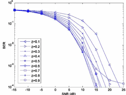
Simulation 5-On Selection of Power Threshold δ : This simulation considers the

optimal precoder (5.13) and illustrates the impact of δ on equalization performance.

Figure 7 shows the bit-error-rate (BER) curves for 0.1≤ ≤δ 0.9; we set K =500, 1000