分析具有奇異應力之功能梯度材料厚版(I)

行政院國家科學委員會專題研究計畫 期中進度報告

分析具有奇異應力之功能梯度材料厚版(1/3)

計畫類別： 個別型計畫 計畫編號： NSC94-2211-E-009-024- 執行期間： 94 年 08 月 01 日至 95 年 07 月 31 日 執行單位： 國立交通大學土木工程學系(所) 計畫主持人： 黃炯憲 報告類型： 精簡報告 處理方式： 本計畫可公開查詢

中 華 民 國 95 年 6 月 1 日

行政院國家科學委員會補助專題研究計畫

□ 成 果 報 告

■期中進度報告

分析具有奇異應力之功能梯度材料厚版 (1/3)

計畫類別：■ 個別型計畫 □ 整合型計畫

計畫編號：NSC 94－2211－E －009 －024 －

執行期間： 94 年 08 月 01 日至 95 年 07 月 31 日

計畫主持人：黃炯憲

共同主持人：

計畫參與人員：張明儒、 廖慎謙

成果報告類型(依經費核定清單規定繳交)：■精簡報告 □完整報告

本成果報告包括以下應繳交之附件：

□赴國外出差或研習心得報告一份

□赴大陸地區出差或研習心得報告一份

□出席國際學術會議心得報告及發表之論文各一份

□國際合作研究計畫國外研究報告書一份

處理方式：除產學合作研究計畫、提升產業技術及人才培育研究計畫、列

管計畫及下列情形者外，得立即公開查詢

□涉及專利或其他智慧財產權，□一年□二年後可公開查詢

執行單位：國立交通大學

中 華 民 國 95 年 05 月 31 日

Abstract

Describing the behaviors of stress singularities correctly is essential for obtaining accurate numerical solutions of complicated problems with stress singularities. This analysis derives asymptotic solutions for functionally graded material (FGM) thick plates with geometrically induced stress singularities. The Reddy’s plate theory is used to establish the equilibrium equations for FGM thick plates. Assuming the Young’s modulus varies along the thickness and constant of Poisson’s ratio, the eigenfunction expansion method is employed to the equilibrium equations in terms of displacement components for an asymptotic analysis in the vicinity of a sharp corner. The characteristic equations for determining the stress singularity order at the corner vertex and the corresponding corner functions are explicitly given for different combinations of boundary conditions along the radial edges forming the sharp corner. The non-homogeneous elasticity properties are present only in the characteristic equations corresponding to boundary conditions involving simple support. Finally, the effects of material non-homogeneity on the stress singularity orders are thoroughly examined by showing the minimum real values of the roots of the characteristic equations varying with the material properties and vertex angle.

Keywords: FGM thick plates, Stress singularities, Asymptotic solutions, Eigenfunction

expansion method 摘要 為獲得複雜的應力奇異性問題的精確數值解，準確地描述應力奇異行為是非常重要 的。本研究以 Reddy 板理論建構功能梯度材料(FGM)厚板之平衡方程式，並推導其幾何 奇異應力之漸近解。本研究假設楊氏模數(Young’s modulus)隨著厚度改變，而波松比 (Poisson’s ratio)則為常數。利用特徵函數展開法求解以位移分量表示之平衡方程式，求 得尖銳角處之漸近解析解。推導對應於不同徑向邊界條件之特徵方程式以決定尖銳角處 應力奇異階數，並進而獲得描述應力奇異行為之特徵函數。結果發現只有含簡支撐徑向 邊界條件之特徵方程式包括非齊性的材料性質；但不管何種徑向邊界條件，材料的非齊 性導致撓曲(bending)與拉伸(extension)行為互為藕合。 關鍵詞： 功能梯度厚板，應力奇異性，漸近解，特徵函數展開法

1. Introduction

Functionally graded materials (FGMs) were first produced in Japan in the mid-1980s (Niino and Maeda, 1990). An FGM is a multi-phase material comprised of different material components, such as ceramics and metals, that have various mixture ratios and microstructures. The gradual variation in material composition rather than sharp interfaces, as in the case of multilayered systems (i.e., laminated composites), significantly enhances the thermal and mechanical features of FGMs. Furthermore, FGMs can be designed to meet particular requirements, such as enhanced stiffness, toughness and resistance to corrosion, wear and high temperature, by using materials or material systems with various properties. Consequently, in the last two decades, FGMs have been used in numerous demanding engineering applications including military armor, thermal barrier coating for turbine blades and internal combustion engines and machine tools.

An FGM plate can be designed with material properties that vary gradually in the thickness direction, such that the plate is non-homogeneous in that direction only. A plate is a widely used component in practical engineering, and has various shapes. A plate with a reentrant corner or V-notch often shows stress singularities at the corner or vertex. These stress singularities must be considered if analysis is to be of real use. Stress singularity behaviors in a problem must be properly considered to obtain a convergent and accurate numerical solution (Leissa et al., 1993; Huang et al., 2005).

Studies of stress singularities resulting from various boundary conditions in angular corners of plates are limited to homogeneous plates or bi-material plates. Williams (1952a and 1952b) first showed the stress singularities of a thin plate under extension or bending due to various boundary conditions. Based on plane elasticity or classical plate theory, several studies used various approaches to investigate stress singularities at the interface corner of a bi-material plate (Hein and Erdogan, 1971; Bogy, 1971; Rao, 1971; Gdoutos and Theocaris, 1975; Dempsey and Sinclair, 1981; Ting and Chou, 1981). Burton and Sinclair (1986), Huang (2002a, 2002b, 2003, 2004), and McGee

et al. (2005) investigated the stress singularities at thick plate corners using different plate theories

or various analytical solution techniques. Based on three-dimensional elasticity, Ba(zantand Estenssoro (1977), Kerr and Parihar (1977), Schmitz et al. (1993), and Glushkov et al. (1999) applied different numerical solution techniques to investigate geometrically induced stress singularities at a three-dimensional vertex of a homogenous body. Somaratna and Ting (1986) and Ghahremani (1991) used a finite element approach to study stress singularities in anisotropic materials and composites. Huang and Leissa (2006) developed three-dimensional corner displacement functions for bodies of revolution.

Although geometrically induced stress singularities on an FGM plate have never been investigated, crack-related problems in FGMs have been frequently studied using plane or three-dimensional elasticity theory. Based on plane elasticity, Delale and Erdogan (1983) and Erdogan (1985) employed integral equation techniques to solve crack problems with mechanical loading, whereas Noda and Jin (1993) and Jin and Noda (1993) considered thermal loading. Furthermore, Erdogan and his coworkers (1988, 1991) investigated interface crack problems in bonded FGM plates. Using three-dimensional elasticity, Gu and Asaro (1997) applied an asymptotic solution of crack tip stress and displacement fields for homogeneous materials to examine small crack deflection in brittle FGMs. Gu et al. (1999), Rousseau and Tippur (2002), Kim and Paulino (2002), and Jin and Dodds Jr (2004) applied different finite element techniques to solve various crack problems. Chen et al. (2000) and Yue et al. (2003) utilized the mesh free Galerkin method and boundary element approach, respectively, to solve various crack problems.

This work examines geometrically induced stress singularities for an FGM plate using Reddy’s thick plate theory. The equilibrium equations in terms of displacement components on the mid-plane are developed for an FGM thick plate. The in-plane displacement components are

coupled with the out-of-plane displacement component in the equations due to the non-homogeneity of an FGM. Asymptotic analysis of stress singularities in the vicinity of a sharp corner is carried out using the eigenfunction expansion approach. By assuming constant Poisson’s ratio along the thickness, the characteristic equations for determining orders of stress singularity at the sharp corner are established for different sets of boundary conditions along the two radial edges forming the corner. The asymptotic solutions for the displacement functions are also explicitly presented. The effects of elasticity modulus variation along the thickness on stress singularity orders are thoroughly examined. These results are the first shown in the published literature.

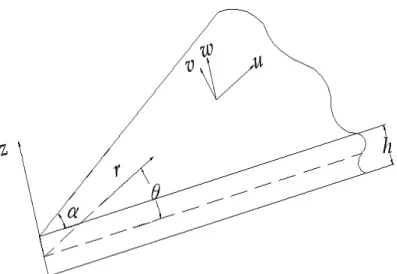
2. Basic formulation

Consider a thick wedge (or sector plate) (Fig.1). The wedge is composed of FGM with material properties varying in the thickness direction (z direction). That is, the wedge is non-homogeneous only in the thickness direction. The displacement field for the wedge with cylindrical coordinates (Fig. 1), based on Reddy’s third-order plate theory, is given as

)] , ( ) , ( ( ) ( 3 4 ) , ( [ ) , ( ) , , ( θ ₀ θ ψ θ 2 ψ r θ w_, r θ h z r z r u z r u = + _r − _r + _r , (1a) )] , ( 1 ) , ( ( ) ( 3 4 ) , ( [ ) , ( ) , , ( θ ₀ θ ψ_θ θ 2 ψ_θ θ w_,θ r θ r r h z r z r v z r v = + − + , (1b) ) , (r θ w w= , (1c)

where u,v, andware the displacement components in r, θ , and z directions, respectively; u , ₀

0

v , and w are the corresponding displacements on the mid-plane; ψ and _r ψ_θare the rotations of the mid-plane normal in the radial and circumferential directions, respectively; the subscript “,j” denotes partial differentials with respect to the independent variable j. This displacement field leads to zero shear stresses, σ and _zr σ_zθ , on the plate top and bottom surfaces.

Introducing the following stress resultants

dz z R Q _h h z ⎭ ⎬ ⎫ ⎩ ⎨ ⎧ = ⎭ ⎬ ⎫ ⎩ ⎨ ⎧

∫

− 1 2 / 2 / β β β _σ , (2a) dz z z P M N h h ⎪⎭ ⎪ ⎬ ⎫ ⎪⎩ ⎪ ⎨ ⎧ = ⎪ ⎭ ⎪ ⎬ ⎫ ⎪ ⎩ ⎪ ⎨ ⎧

∫

− 3 2 / 2 / 1 ββ β β β σ , (2b) dz z z P M N h h r r r r ⎪⎭ ⎪ ⎬ ⎫ ⎪⎩ ⎪ ⎨ ⎧ = ⎪⎭ ⎪ ⎬ ⎫ ⎪⎩ ⎪ ⎨ ⎧

∫

− 3 2 / 2 / 1 θ θ θ θ σ (2c)

where σ_ij are stress components, and using the principle of stationary potential energy, one can obtain the equilibrium equations without external loading (cf. Reddy, 1999)

0 / ) ( / , , +N r+ N −N r = N_{rr rθθ r θ} , (3a) 0 / 2 / , , +N r+ N r= N_{rθ r θθ rθ} , (3b) 0 1 ) 2 2 1 1 2 ( _{, , ,} 2 , , , 2 , , 1 + + θ θθ − θ + θ θ + θ θ + + + Qθ θ = r Q r Q P r P r P r P r P r P C _{rrr r r r r r r} r _rr , (3c) 0 1 , , + − + r − r = r r r M Q r r M r M M θ _{θθ , (3d)}

0 2 1 , , + + − θ = θ θ θ θ _r Q M M M r r r r , (3e) where 2 1 3 4 h C = , 2 2 4 h C = ,M_rθ =M_rθ −C₁P_rθ , M_β =M_β −C₁P_β , Q_β =Q_β −C₂R_β , h is the thickness of plate and subscript β denotes r or θ. In addition, the following boundary conditions along θ =α should be specified:

0 u or N , _rθ v or ₀ N , _θ ψ_θ or M , _θ ψ_r or M , _rθ w or _{θ 1}(2 _θ 2 _θ, 1P_θ,θ) r P P r C Q + _r + _{r r} + , and r w_,θ or P . (4a) _θ

The circumferential boundary conditions (at r=R) should prescribe:

0 u or N_r, v or ₀ N ,_rθ ψ_θ or M , _rθ ψ_r or M , _r w or ₁( _, 2 _, ) r P P r P r P C Q_r + r + _rr + _{rθ θ} − θ , and w_,r or P_r. (4b) For an isotropic and elastic plate, the relationships between the stress resultants and

displacement components are established by using strain-displacement and stress-strain relationships. They are,

θθ θ 1 3 , 1 3 , 1₂3 , , 0 0 , 0 0 0 0 _w r D C w E C w r D C v r D u E u r D N_r = + _r + − _r − _rr θ θ ψ ψ ψ _{1 1 3 , 1 1 3 ,} 3 1 1 ( ) 1 ) ( ) ( 1 D C D r E C E D C D r − r + − rr + − + ， (5a) θθ θ θ 0 0 0 0, 0 0, 1 3 , 1 3 , 1₂3 w, r E C w D C w r E C v r E u D u r E N = + _r + − _r − _rr − 1( _{1 1 3})ψ ( _{1 1 3})ψ _, 1(E₁ C₁E₃)ψ_θ,θ r D C D E C E r − r + − rr + − + ， (5b) θ θ θ θ r r r w r G C w r G C v G v r G u r G N 1 3 _, , 2 3 1 , 0 0 0 0 , 0 0 _{− + +}2 ₋2 = ) ) ( 1 )( ( _{1 1 3 r, ,r} r G C G − ψ _θ −ψ_θ +ψ_θ + ， (5c) ) )( ( _{0 2 2 r ,r} r G C G w Q = − ψ + ， (5d) ) 1 )( ( _{0 2 2 θ ,θ} θ ψ w r G C G Q = − + ， (5e) ) )( ( _{2 2 4 r ,r} r G C G w R = − ψ + ， (5f) ) 1 )( ( _{2 2 4 θ ,θ} θ ψ w r G C G R = − + ， (5g) θθ θ 1 4 , 1 4 , 1₂4 , , 0 1 , 0 1 0 1 _w r D C w E C w r D C v r D u E u r D M_r = + _r + − _r − _rr 1( _{2 1 4})ψ ( _{2 1 4})ψ _, 1(D₂ C₁D₄)ψ_θ,θ r E C E D C D r − r + − rr + − + ， (5h) θθ θ θ 1 0 1 0, 1 0, 1 4 , 1 4 , 1₂4 w, r E C w D C w r E C v r E u D u r E M = + _r + − _r − _rr −

1( _{2 1 4})ψ ( _{2 1 4})ψ _, 1(E₂ C₁E₄)ψ_θ,θ r D C D E C E r − r + − rr + − + ， (5i) θ θ θ θ r r r _r w G C w r G C v G v r G u r G M 1 4 _, , 2 4 1 , 0 1 0 1 , 0 1 _{− + +}2 ₋2 = ( _{2 1 4})(1( _r, ) _,r) r G C G − ψ _θ −ψ_θ +ψ_θ + ， (5j) θθ θ 1 6 , 1 4 , 1₂6 , , 0 3 , 0 3 0 3 _w r D C w E C w r D C v r D u E u r D P_r = + _r + − _r − _rr 1( _{4 1 6})ψ ( _{4 1 6})ψ _, 1(D₄ C₁D₆)ψ_θ,θ r E C E D C D r − r + − rr + − + ， (5k) θθ θ θ 3 0 3 0, 3 0, 1 6 , 1 6 , 1₂6 w, r E C w D C w r E C v r E u D u r E P = + _r + − _r − _rr − 1( _{4 1 6})ψ ( _{4 1 6})ψ _, 1(E₄ C₁E₆)ψ_θ,θ r D C D E C E r − r + − rr + − + ， (5l) θ θ θ θ r r r _r w G C w r G C v G v r G u r G P 1 6 _, , 2 6 1 , 0 3 0 3 , 0 3 _{− + +}2 ₋2 = ( _{4 1 6})(1( _r, ) _,r) r G C G − ψ _θ −ψ_θ +ψ_θ + ， (5m) where dz Gz G h h i i

∫

− = 2 / 2 / ， E E z dz h h i i

∫

− − = 2 / 2 / 2 1 υ ， z dz E D h h i i

∫

− − = 2 / 2 / 2 1 υ υ ， (5n) and G, E, and υ are shear modulus, modulus of elasticity, and Poisson’s ratio, respectively, all of

which can be functions of z. Since the variation range of Poisson’s ratio is small and the stress singularity order at the interface corner in a bi-material isotropic plate is not sensitive to Poisson’s ratio (Huang, 2002a), the Poisson’s ratio is assumed constant through the thickness in the following. Then, D , _i E , and _i G defined in Eq. (5n) satisfy the following relations: _i

i i E D =υ and G_i E_i 2 ) 1 ( −υ = . (6)

Substituting Eqs. (5a-5m) and (6) into Eqs. (3a-3e) yields the equilibrium equations for displacement functions as ) 2 1 2 3 2 1 ( _{0, 0,} 2 , 0 2 , 0 , 0 2 0 0 θθ θ θ υ υ υ r rr r _v r v r u r u r u r u E − + + + − − − + + + ) 2 3 ( 2 , , 3 , , 2 , 3 1 r w w r w r w r w E C r − rr − _rrr + +υ _θθ − rθθ + r rr _rrr r r E C E , _, 2 3 1 1 )( ( − ψ +ψ +ψ + ) 0 2 1 2 3 2 1 , , 2 , 2 = + + − − − θ θ θ θ θθ υψ υψ ψ υ r r _r r r ， (7a) ) 2 1 2 1 2 1 2 1 2 3 ( 2 , 0 , 0 , 0 0 2 , 0 , 0 2 0 r v v v r v r u r u r E −υ _θ + +υ _rθ − −υ + −υ _r + −υ _rr + θθ + rθ υ _rrθ θθθ υψ_rθ υψ_rrθ r r E C E r w w r r w E C _{, ,} 2 3 1 1 3 , , 2 , 3 1 2 1 2 3 )( ( ) 2 1 (− − + − + − − + +

) 0 2 1 2 1 2 1 2 , , , 2 + = − + − + − − r r r r rr θθ θ θ θ θ ψ ψ υ ψ υ ψ υ ， (7b) ) 2 ( 2 , 0 3 , 0 , 0 , 0 , 0 , 0 2 , 0 , 0 3 , 0 0 3 1 r u r v u u r v u r v u r v u E C + θ − r + rθ + rr + rrθ + _rrr + θθ + θθθ + rθθ + ( 4 2 2 2 _, ) 2 , 4 , , 3 , 4 , 2 , 3 , 6 2 1 rrrr rr rrr r rr r _w r w r w r w r w r w r w r w E C − + − θθ + θθ − − θθθθ − θθ − + ( 2 )( ) 2 1 , , , , 4 2 2 2 2 0 r r w r w E C E C E r _rr ψr ψ_rr ψθθ υ _{− + + + + +} − + 3 , , 2 , , 3 , 6 2 1 4 1 )( ( r r r E C E C − ψr +ψθθ −ψrr +ψθ rθ +ψrθθ +ψθθθθ 0 ) 2 , 2 , , , + _{+ + =} + rrr rr rr _rrrr r r ψ ψ ψ ψ _{θ θ θθ} ， (7c) ) 2 1 2 3 2 1 )( ( 0, 2 0, 2 0, 0, , 0 2 0 3 1 1 θθ θ θ υ υ υ r rr r _v r v r u r u r u r u E C E − − + + + − − − + + +( )( 2 ) 2 , , 3 , , 2 , 6 2 1 4 1 r w w r w r w r w E C E C − r − rr + θθ − _rrr − rθθ + + + − − − ( 2 )( ) 2 1 , 4 2 2 2 2 0 C E C E wr r E ψ υ 0 ) 2 1 2 3 2 1 )( 2 ( _{, ,} 2 , , 2 , 2 6 2 1 4 1 2 = + + − − + − + + − + − ψr ψrr υψ_rθθ ψ_rrr υψ_θθ υψ_{θ rθ} r r r r r E C E C E ， (7d) ) ) ( 2 1 2 1 2 3 )( ( 2 , 0 , 0 , 0 2 0 , 0 , 0 2 3 1 1 r v v r v r v u r u r E C E − −υ _θ + +υ _rθ − −υ − r − _rr + θθ ) )( 2 ( 2 1 ) )( ( , _{0 2 2 2}2 ₄ , 3 , 2 , 6 2 1 4 1 θ θ θ θθθ θ _{+ + −} −υ _{− + +ψ} − − r w E C E C E r w r w r w E C E C r rr + υψ _θ υψ _θ υψ_θ 2 , , 2 6 2 1 4 1 2 2 1 2 1 2 3 )( 2 ( r r r E C E C E − + − _r + + _rr − − 0 ) 2 1 2 1 , 2 , , = − + + − + _{r rr} r r θ θθ θ θ υψ ψ ψ υ ， (7e)

Apparently, the in-plane displacement components u and₀ v are coupled with out-of-plane ₀ displacement w in the mid-plane.

3. Asymptotic solutions

The eigenfunction expansion approach proposed by Hartranft and Sih (1969) for three-dimensional elasticity problems is adopted herein to find the solution of Eqs. (7a-7e). The displacement components can be expressed in terms of the following series

) , ( ) , ( ( ) 0 0 0 ni i i n n_U r r u θ

∑∑

λi θ λ ∞ = ∞ = + = ， ( , ) ()( , ) 0 0 0 i i n i n n_V r r v θ

∑∑

λi θ λ ∞ = ∞ = + = ， ) , ( ) , ( () 0 0 1 i i n i n n _W r r w θ

∑∑

λi θ λ ∞ = ∞ = + + = ， ( , ) ()( , ) 0 0 i i n i n n r r θ r i θ λ ψ ₌

∑∑

∞ λ _Ψ = ∞ = + ，

) , ( ) , ( () 0 0 i i n i n n i r r θ θ λ ψ_θ =

_{∑ ∑}

∞ λ Φ = ∞ = + _{， (8)}

where the characteristic valuesλ_i are assumed to be constants and can be complex numbers.

The real part of λ_i must exceed zero to satisfy the regularity conditions at the vertex of the sector plate. The regularity conditions require that u , ₀ v , ₀ ψ_θ , ψ , w and _r w_,r are finite as r approaches zero. As a result, the solution form given in Eq. (8) with the real part of λ_iless than one leads to singularities of N_r, N , _θ N ,_rθ M_r,M_θ,M_rθ,P_r ,P_θ andP_rθ , which is observed from the relationships between stress resultants and displacement components given in Eqs. (5a-5m). However, no singularity for shear forces (Q_r ), andQ_θ R_r and R will be produced from the _θ solution.

Substituting Eq. (8) into Eqs. (7a-7e) and considering those solutions corresponding to the lowest order of r, which dominate the stress singularity features at the neighborhood of r=0, yield

(

)

[

]

() , 0 0 ) ( , 0 0 ) ( 0 0 2 1 2 3 2 1 1 1 _{i i i} U i E U i _i E V i E λ λ λ υ _θθ υ υ λ ⎟ _θ ⎠ ⎞ ⎜ ⎝ ⎛₋ − ₊ + + − + − + + − +C₁E₃

[

λ_i +1−λ_i

(

λ_i +1

) (

− λ_i +1

) (

λ_i λ_i −1

)

]

W₀(i)+C₁E₃

[

2−

(

λ_i +1

)

]

W₀(_,θθi) +

(

_{1 1 3}

)

[

(

)

]

₀()

(

_{1 1 3}

)

₀(_,) 2 1 1 1 _{i i} i i i E C E E C E − λ − +λ λ − Ψ + − −υ Ψ _θθ +

(

)

0 2 1 2 3 () , 0 3 1 1 ⎟Φ = ⎠ ⎞ ⎜ ⎝ ⎛₋ − ₊ + − i i E C E υ υ λ _θ , (9a)

(

)

[

]

() , 0 0 ) ( 0 0 ) ( , 0 0 1 1 2 1 2 1 2 3 i i i i i i i U E V E V E υ υλ ⎟ _θ + −υ λ − +λ λ − + _θθ ⎠ ⎞ ⎜ ⎝ ⎛ − ₊ + + _{1 3}

[

(

)

(

)

]

₀(_,) _{1 3 0}(_,)

(

_{1 1 3}

)

₀(_,) 2 1 2 3 1 2 1 _{i i} i i _i i i W C E W E C E E C λ λ λ _{θ θθθ} υ υλ ⎟Ψ _θ ⎠ ⎞ ⎜ ⎝ ⎛ − ₊ + − + − + − + − +

(

)

[

1

(

1

)

]

(

)

0 2 1 () , 0 3 1 1 ) ( 0 3 1 1 − + − Φ + − Φ = − −C E _{i i i} i E C E i E υ λ λ λ _θθ , (9b)

(

)

( ) , 0 3 1 ) ( 0 2 3 1 ( 1) ( 1) 1 i i i i i U C E U E C λ − λ + + λ + _θθ -C₁2E₆(λ_i +1)2 (λ_i −1)2W₀(i) +C₁2E₆

[

−4+2

(

λ_i +1

)

−2λ_i

(

λ_i +1

)

]

W₀(_,i_θθ) −C₁2E₆W₀(_,i_θθθθ) +

(

C₁E₄ −C₁2E₆

)

(λ_i −1)2 (λ_i +1)Ψ₀(i) +

(

C₁E₄ −C₁2E₆

)

(

λ_i +1

)

Ψ_0,θθ(i) +

(

C₁E₄−C₁2E₆

)

(λ_i −1)2Φ₀(i_,)_θ +

(

C₁E₄ −C₁2E₆

)

Φ_0,θθθ(i) =0, (9c)

(

)

(

)

( ) , 0 3 1 1 ) ( 0 3 1 1 2 1 ) 1 )( 1 (λ_{i i} U i E C E U i E C E − − λ + + −υ − _θθ +

(

_{1 1 3}

)

₀(_,) 2 1 2 3 i i V E C E υ υλ ⎟ _θ ⎠ ⎞ ⎜ ⎝ ⎛₋ − ₊ + − -

(

C₁E₄−C₁2E₆

)

(λ_i +1)2(λ_i −1)W₀(i)

(

)

(

)

() , 0 6 2 1 4 1 1 i i W E C E C − −λ _θθ +

(

)

() 0 6 2 1 4 1 2 2 ( 1)( 1) i i i E C E C E − + + − Ψ + λ λ +

(

)

) 0 2 1 2 3 2 1 ( 2 _{1 4 1}2 _{6 0}(_,) (_0,) 2 ⎟Φ = ⎠ ⎞ ⎜ ⎝ ⎛ + + − − + Ψ − + − C E C E i _i i E υ _θθ υ υλ _θ , (9d)

(

_{1 1 3}

)

₀(_,)

(

_{1 1 3}

)

( 1)( 1) ₀() 2 1 2 1 2 3 i i i i i U E C E V E C E ⎟ + − − + − ⎠ ⎞ ⎜ ⎝ ⎛ + + − − υ υλ _θ υ λ λ

+

(

E₁−C₁E₃

)

V₀(_,i_θθ) −

(

C₁E₄−C₁2E₆

)

(

λ

_i+1)2W₀(_,i_θ)−

(

C₁E₄−C₁2E₆

)

W₀(_,i_θθθ)

(

)

() , 0 6 2 1 4 1 2 2 1 2 3 2C E C E _i i E υ υλ ⎟Ψ _θ ⎠ ⎞ ⎜ ⎝ ⎛ + + − + − +

(

)

) ] 0 2 1 2 1 [( 2 _{1 4 1}2 ₆ 2 (₀) (_0,) 2 Φ +Φ = − + − − + − + i i i E C E C E υ υλ _θθ . (9e)

Equations (9) are a set of linear differential equations with constant coefficients. Following a typical procedure for solving a set of linear differential equations, the general solutions for

) ( 0 ) ( 0 ) ( 0 , and i i i _{V W} U are obtained as θ λ θ λ θ λ θ λ λ

θ, ) cos( 1) sin( 1) cos( 1) sin( 1)

( _{i 2 3 4} ) ( 0 = ₁ i + + i + + i − + i − i _{A A A A} U , (10a)

(

κ κ

)

λ θ θ λ θ λ λ

θ, ) cos( 1) sin( 1) cos( 1)

( i _{2 1 1 4 2 4} ) ( 0 = i + − i + + − i − i _{A A A B} V

(

−κ_{1 3} κ_{2 3}

)

sin(λ −1)θ + A ＋ B _i , (10b) θ λ θ λ θ λ θ λ λ

θ, ) cos( 1) sin( 1) cos( 1) sin( 1)

( _{1 2 3 4} ) ( 0i i =B i + +B i + +B i − +B i − W , (10c) θ λ θ λ θ λ θ λ λ

θ, ) cos( 1) sin( 1) cos( 1) sin( 1)

( _{1 2 3 4} ) ( 0 = + + + + − + − Ψ i _{i D i D i D i D i} , (10d)

(

κ κ

)

λ θ θ λ θ λ λ

θ, ) cos( 1) sin( 1) cos( 1)

( _{2 1 1 4 3 4} ) ( 0 = + − + + − − Φ i _{i D i D i D B i} +

(

−κ₁D₃ +κ₃B₃

)

sin(λ_i −1)θ , (10e) where υ λ υ λ υ λ υ λ κ i i i i + + + − + − + = 3 3 1 ,

(

)

(

)

(

)

υ λ υ λ λ κ i i i E C E C E E E C E E C E E C E E E E C E E C + + + − + − − + − + − + − − = 3 2 2 8 6 2 1 4 1 2 0 2 3 2 1 3 1 1 2 1 6 1 4 1 4 3 1 3 2 1 2 and

(

)

(

)

(

)

υ λ υ λ λ κ i i i E C E C E E E C E E C E E C E E E C E E C + + + − + − − + − + − + − = 3 2 2 8 6 2 1 4 1 2 0 2 3 2 1 3 1 1 2 1 6 1 4 0 2 3 1 3 1 1 3 .

Coefficients Ai, Bi and Di (i=1, 2, 3, 4) and λi are to be determined from boundary conditions along the radial edges. Notably, the extension and bending of a plate will be independent when E ₁ and E equal zero. ₃

4. Boundary conditions, characteristic equations and corner functions

After solving the equilibrium equations, attention is now turned to find out Ai, Bi, Di and λi in the solutions from the boundary conditions along the radial edges forming a corner. To determine Williams type stress singularities at the vertex of a sector plate caused by homogeneous boundary conditions, one only needs the asymptotic solution with the lowest order of r in the series solution of Eq.(8). Consequently, only the solution with n=0 in Eq. (8) needs to be considered. Let,

) , ( ) ( 0 ) ( 0 m m m _{r U} u = λm θ λ _, ( )_{( , )} 0 ) ( 0 m m m _{r V} v = λm θ λ ) , ( ) ( 0 ) ( 0 m m m _{r mΦ θ λ} ψ_θ = λ , )ψ_r(m₀) =_rλmΨ₀(m)(θ,λ_{m , and} ( )_{( , )} 0 1 ) ( 0 m m m _{r W} w = λm+ θ λ ₍₁₁₎

Furthermore, as well known, the stress singularities are affected by the boundary conditions along radial edges only.

radial edge, say θ =α , namely, clamped: ₀ = ₀ = = = = , =0 r w w v u ψ_r ψ_θ θ , (12a) free: _θ = _θ = _θ = _θ = _θ + ₁(2 _θ +2 _θ, +1P_θ,θ)=P_θ =0 r P P r C Q M M N N_{r r r r r} , (12b)

type I simply supported: u₀ =v₀ =w=ψ_r =M_θ =P_θ =0, (12c) type II simply supported: u₀ =v₀ =w=M_θ =M_rθ =P_θ =0. (12d) For the simplicity, C and F are used to present the clamped and free boundary conditions,

respectively, while S(I) and S(II) denote type I and type II simply supported boundary conditions. For the sake of demonstration, we will describe the procedure for obtaining the characteristic equation for λ_m, and the corresponding asymptotic displacement field for describing the singular behavior of stress resultants in the vicinity of a corner. A wedge with simply supported radial edges and a vertex angle α is utilized to demonstrate a typical procedure for deriving these coefficients and λ . S(I) boundary conditions simulate the mechanical support of a knife-edge along the mid-plane. By taking advantage of the problem’s symmetry, the solutions given in Eq. (11) are separated into symmetric and anti-symmetric parts. The symmetric solutions satisfying the boundary conditions yield

(

)

(

)

0 2 1 cos 2 1 cos ₃ 1 + + − = α λ α λ_m A _m A ,

(

)

0 2 ) 1 sin( 2 ) 1 sin( _{1 3 2 3} 1 + + − = −A λ_m α －κ A＋κ B λ_m α , 0 2 ) 1 cos( 2 ) 1 cos( ₃ 1 + + − = α λ α λ_m B _m B , 0 2 ) 1 cos( 2 ) 1 cos( ₃ 1 + + − = α λ α λ_m D _m D ,

(

)

(

)

(

)

2 1 cos } 1 ) ( { 1 _{1 1 1 2 1 4 1 1 4} λ λ α λ_m + −A E +D −E +C E +BC E _m + _m +

(

)

(

)

(

)

0 2 1 cos } 1 ( ) ( { 1 − _{3 1 1}+ ₁ − ₂ + _{1 4 3}+ _{2 1}+ _{3 4} − _{1 4} + ₃ − ₃ − = − + λ_m A κ E κ E C E D κ E κ E C E κ λ_m B λ_m α

(

)

(

)

(

)

2 1 cos } 1 ) ( { 1 _{1 3 1 4 1 6 1 1 6} λ λ α λ_m + −A E +D −E +C E +BC E _m+ _m +

(

)

(

)

(

)

0 2 1 cos } 1 ( ) ( { 1 − _{3 1 1}+ ₁ − ₄ + _{1 6 3}+ _{2 3} + _{3 4} − _{1 6} + ₃− ₃ − = − + λ_m A κ E κ E C E D κ E κ E C E κ λ_m B λ_m α (13) Equations (13) are a set of six linear algebraic equations for Ai, Bi and Di (i=1 and 3). To have nontrivial solutions for these coefficients yields a 6th order determinant equal to zero, which leads to

(

)

0 2 1 cos λ_m + α = ,

(

)

0 2 1 cos λ_m − α = , (14a) or γ₁λ_msinα+sinλ_mα =0 (14b) where 2 1 1 _κ κ γ = , κ₁=

[

−C₁E₄(−κ₂E₃+2(1+κ₁)E₄)+κ₂E₁(E₄−C₁E₆)+E₂(−κ₂E₃+2C₁(1+κ₁)E₆)

]

,

[

_{1 4}( _{2 3} 2( 1 ₁) ₄) _{2 1}( _{4 1 6}) ₂( _{2 3} 2 ₁( 1 ₁) ₆)

]

2 C E κ E κ λmE κ E E C E E κ E C κ λmE κ = − + − + − − − − + − + . When λ_m satisfies

(

)

0 2 1 cosλ_m + α = and

(

)

0 2 1

Di (i=1 and 3) are obtained from Eq. (13). Then, the corresponding asymptotic solutions are

(

)

{

λ θ

}

λ 1 cos 1 1 ) ( 0 = + + m m _{B r m} w , ψ_r(m₀) =_D1rλm

{

cos

(

λ_m +1

)

θ

}

_, ψ λ

{

(

λ

)

θ

}

θ 1 sin 1 ) ( 0 = − m+ m _{D r m} . (15) The asymptotic solutions for u₀(m)and v₀(m) have the order of r larger than λ_m and do not cause stress singularities. These asymptotic solutions given in Eq. (15) are also called corner functions corresponding to the characteristic equation

(

)

0

2 1

cos λ_m + α = . The asymptotic solutions for in-plane and out-of-plane displacement components on the mid-plane are independent.

Similarly, one can find the corner functions corresponding to different characteristic equations

(i.e.,

(

)

0

2 1

cos λ_m − α = or γ₁λ_msinα+sinλ_mα =0in Eqs. (14)), which are listed in Table 1.

Notably,

(

)

0 2 1 cosλ_m− α = and

(

)

0 2 1

cos λ_m + α ≠ yields the asymptotic solution for v₀(m) with the order of r larger than λ_m, which is not given in Table 1.

Using the anti-symmetric parts of solutions in Eq. (11) and following the procedure above, the following characteristic equations are easily established:

(

)

(

)

) 0 2 1 )(sin 2 1 (sin λ_m + α λ_m − α = , (16a) or 0 sin sinλ_mα −γ₁λ_m α= . (16b)

The corner functions corresponding to these characteristic equations are also given in Table 1. Notably,

(

)

) 0 2 1 (sin λ_m + α = and

(

)

) 0 2 1

(sin λ_m− α ≠ also yield the asymptotic solutions for u₀(m) and v₀(m) having the order of r larger than λ_m , while

(

)

) 0

2 1 (sin λ_m − α = and

(

)

) 0 2 1

(sin λ_m + α ≠ gives the asymptotic solution for v₀(m) with the order of r larger than λ_m. These asymptotic solutions do not yield stress singularities and are not listed in Table 1.

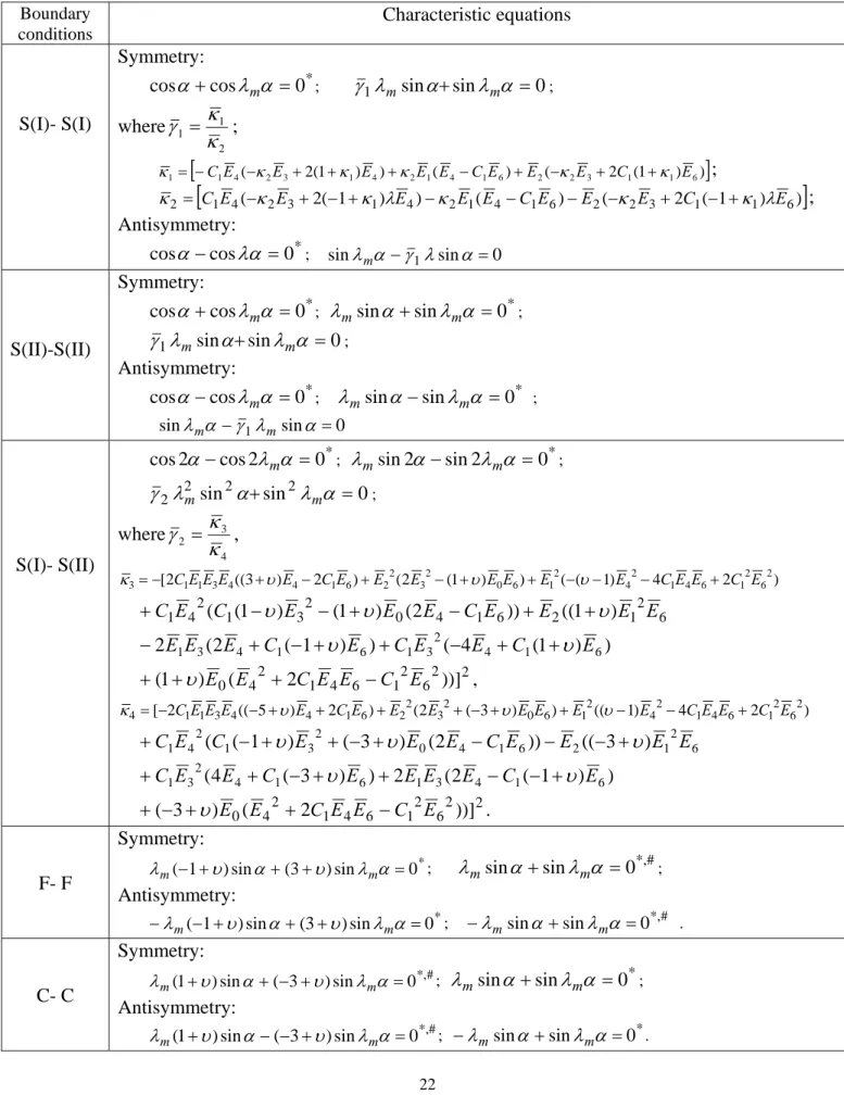
Characteristic Eqs.(14a) and (16a) do not involve material properties, and are identical to the characteristic equations for a homogeneous thick sectorial plate with two simply supported radial edges under bending. However, material properties are involved in the characteristic equations Eqs.(14b) and (16b).

By following the procedure given above, one can develop the characteristic equations for λ_m and the corresponding corner functions for different boundary conditions along radial edges. Table 2 summarizes the characteristic equations for λ_m for eight different combinations of boundary conditions. To take advantage of the problem’s symmetry, the corner functions for the identical boundary conditions along two radial edges were determined by considering the range,

2 / 2

/ θ α

α ≤ ≤

− . Table 1 summarizes the corner functions for S(I)_S(I), S(II)_S(II), C_C and F-F, which are already considerably complicated. The corner functions corresponding to other boundary conditions are too lengthy and complicated to be given in Table 1. These results given in Tables 1 and 2 are the first shown in the published literature.

Notably, Table 2 does not list the characteristic equations for S(I)_F and S(II)_F boundary conditions because they are much more complicated and lengthy than those given in Table 2. To find the values ofλ_m for these boundary conditions, it is suggested to determine them directly from solving the zeros of the 12th order determinant established from S(I)_F or S(II)_F boundary conditions.

without involving S(I) or S(II) condition are identical to the combination of the characteristic equations for homogeneous plates under bending and extension (Williams (1952a), Huang (2002)). The non-homogeneity considered here does not influence the stress singularity orders at the corner of a plate if one of the two radial edges around the corner is not simply supported. However, Table 1 shows that most of the asymptotic solutions for the in-plane and out-of-plane displacement components on the mid-plane are coupled and are significantly different from those for homogenous plates.

5. Numerical results for λ_m

To demonstrate the effects of material non-homogeneity on stress singularity orders, a typical non-homogeneity is considered, assuming the variations of the Young’s modulus through the thickness of plate given as

(z) )

(z E V E

E = _b + ∆ , (17)

where V(z)=(z/h+1/2)m. Consequently, the roots of the characteristic equations corresponding to boundary conditions involving simple support (see Table 2) depend on m, υ and ∆E /E_b. The Poisson’s ratio is set equal to 0.3 for the results shown below.

Figure 2 depicts the variation of the minimum real parts of λ_m (Re[λ ], the subscript m is omitted for simplicity) with the material properties and the vertex angle of a wedge having S(I)_S(I) boundary conditions along radial edges. The roots of Eqs. (14a), (14b), (16a), and (16b) were obtained independently. An infinite number of roots exist for each of these equations. Only the root with a minimum real part is important as it determines the stress singularity order at the vertex. The minimum values of Re[λ ] obtained from Eq. (14a), independent of material properties, are smaller than those for Eq. (14b) for a wide range of material properties when minimum Re[λ ] is less than unity. Similarly, minimum values of Re[λ ] determined from Eq.(16a) are less than those for Eq. (16b) with different material properties. As a result, the singularity order of the stress resultants at a sharp corner with S(I)_S(I) edges is very likely determined by Eq. (14a) or (16a), independent of material properties.

Figures 3and 4 illustrate the effects of material non-homogeneity on the minimum values of Re[λ ] of the characteristic equations corresponding to S(I)_S(II) and S(I)_C boundary conditions, respectively. Since the characteristic equation involving material non-homogeneity for S(II)_C boundary conditions is the same as that for S(I)_C boundary conditions, Fig. 4 also illustrates the minimum values of Re[λ ] of the characteristic equations for S(II)_C boundary conditions. Table 2 reveals that characteristic equations without involving material non-homogeneity were found for S(I)_S(II), S(I)_C and S(II)_C boundary conditions. These characteristic equations are also found for homogeneous plates under bending (Huang (2002)). The results denoted as “homogenous” in Figs. 3 and 4 are the minimum values of Re[λ ] for these characteristic equations without involving material non-homogeneity. The material non-homogeneity considered in these figures does not significantly affect the stress singularity order at the vertex. The stress singularity order is mainly determined by the roots of the characteristic equations corresponding to a homogeneous plate under bending.

Figures 5 and 6 demonstrate the effects of material non-homogeneity on the minimum values of Re[λ ] of the characteristic equations corresponding to S(I)_F and S(II)_F boundary conditions, respectively. The roots of λ_m were determined from the zeros of the 12th order determinant established based on S(I)_F or S(II)_F boundary conditions. It was revealed that no root of λ_m is identical to that obtained from the characteristic equations for a homogenous. Figures 5 and 6 explore that material non-homogeneity significantly affects the stress singularity order at a corner with S(I)_F or S(II)_F boundary conditions along the two edges forming the corner.

6. Concluding remarks

This study has developed the equilibrium equations in terms of displacement functions for an FGM thick plate based on Reddy’s plate theory and established the asymptotic displacement field to describe the singular behaviors of stress resultants in the vicinity of a sharp corner. The asymptotic solutions were obtained using the eigenfunction expansion method and assuming non-homogeneous Young’s modulus and constant Poisson ratio along plate thickness. This work has also established the characteristic equations for determining stress singularity orders at the vertex of the corner with different boundary condition combinations. These asymptotic solutions and characteristic equations are the first given in the literature. Only the characteristic equations corresponding to boundary conditions involving simple support depend on material non-homogeneity. Nevertheless, regardless of the boundary conditions considered, the asymptotic solutions of in-plane and out-of-plane displacement components on the mid-plane are usually coupled.

In examining how material non-homogeneity affects stress singularity orders, this work considered the non-homogeneous Young’s modulus following a power law. The present study considered S(I)_S(I), S(I)_S(II), S(I)_C, S(II)_C, S(I)_F and S(II)_F boundary conditions along the radial edges of a sector plate. The material non-homogeneity considered in the work does not significantly affect the stress singularity order at the vertex when S(I)_S(I), S(I)_S(II), S(I)_C, S(II)_C boundary conditions are considered. The stress singularity order is mainly determined by the roots of the characteristic equations corresponding to a homogeneous plate under bending. However, the material non-homogeneity does significantly affect the stress singularity order at a corner with S(I)_F or S(II)_F boundary conditions along the two edges forming the corner..

The corner functions shown here will be utilized in future FGM plate studies involving geometrically induced stress singularities to determine accurate free vibration frequencies and mode shapes of thick plates having such boundary discontinuities. Because other corner functions have been used advantageously for vibration studies of homogeneous plates (Huang et al., 2005), the present corner functions are definitely appropriate for FGM thick plate vibration problems. These corner functions can also be used for static stress and deformation analysis, especially for determining the stress intensity factors for a V-notch or a crack.

References

ant z

Ba( ,Z. P., Estenssoro, L. F., 1977. General numerical method for three-dimensional singularities in cracked or notched elastic solids. Proceedings of the 4th International Conference on Fracture, Eaterloo, Ontario, 3, 371-385.

Bogy, D. B.,1971. Two edge-bonded elastic wedges of different materials and wedge angles under surface tractions. Journal of Applied Mechanics, 38(2), 377-386.

Burton, W. S. and Sinclair, G. B., 1986. On the Singularities in Reissner’s Theory for the Bending of Elastic Plates. Journal of Applied Mechanics 53, 220-222.

Chen, J., Wu, L., Du, S., 2000. Modified J integral for functionally graded materials. Mechanics Research Communications 27, 301-306.

Delale, F., Erdogan, F., 1983. The crack problem for a nonhomogeneous plane. Journal of Applied Mechanics 50, 609-614.

Delale, F., Erdogan, F., 1988. Interface crack in a nonhomogeneous elastic medium. International Journal of Engineering Science 26, 559-568.

Dempsey, J. P., and Sinclair, G. B., 1981. On the singular behavior at the vertex of a bi-material wedge, Journal of Elasticity 11(3), 317-327.

Erdogan, F., 1985. The crack problem for bonded nonhomogeneous material under antiplane shear loading. Journal of Applied Mechanics 52, 823-828.

materials. Journal of Applied Mechanics 58, 410-418.

Gdoutos, E. E., Theocaris, P. S., 1975. Stress concentrations at the apex of a plane indenter acting on an elastic half-plane. Journal of Applied Mechanics 42(3), 688-692.

Ghahremani, F., 1991. A numerical variational method for extracting 3D singularities. International Journal of Solids and Structures 27(11), 1371-1386.

Glushkov, E., Glushkova, N., Lapina, O., 1999. 3-D elastic stress singularity at polyhedral corner points. International Journal of Solids and Structures 36(8), 105-1128.

Gu, P., Asaro, R. J., 1997. Crack deflection in functionally graded material. International Journal of Solids and Structures 34, 3085-3098.

Gu, P., Dao, M., Asaro, R. J., 1999. A simplify method for calculating the crack-tip field for functionally graded materials using the domain integral. Journal of Applied Mechanics 66, 101-108.

Hartranft, R. J., Sih, G. C., 1969. The use of eigenfunction expansions in the general solution of three-dimensional crack problems. Journal of Mathematics and Mechanics, 19(2), 123-138. Hein, V. L., Erdogan, F., 1971. Stress singularities in a two-material wedge. International Journal of

Fracture Mechanics 7(3), 317-330.

Huang, C. S., 2002a. Corner singularities in bi-material Mindlin plates. Composite Structures 56, 315-327.

Huang, C. S., 2002b. On the singularity induced by boundary conditions in a third-order thick plate theory. Journal of Applied Mechanics 69, 800-810.

Huang, C. S., 2003. Stress singularities at angular corners in first-order shear deformation plate theory. International Journal of Mechanical Science 45(1), 1-20.

Huang, C. S., 2004. Corner stress singularities in a high-order plate theory”, Computers &

Structures 82, 1657-1669.

Huang, C. S., Leissa, A. W., Chang, M. J., 2005. Vibrations of skewed cantilevered triangular, trapezoidal and parallelogram Mindlin plates with considering corner stress singularities. International Journal for Numerical Methods in Engineering 62, 1789-1806.

Huang, C. S., Leissa, A. W., 2006. Three-dimensional sharp corner displacement functions for bodies of revolution. Journal of Applied Mechanics (accepted).

Jin, Z. –H., Noda, N., 1993. Minimization of thermal stress intensity factors for a crack in a metal-ceramic mixture. Ceramic Transations 34: Functionally Gradient Materials, J. B. Holt et al., eds., The American Ceramic Society, Westerville, OH, 47-54.

Jin, Z. –H., Dodds Jr., R. H., 2004. Crack growth resistance behavior of a functionally graded material: computational studies. Engineering Fracture Mechanics 71, 1651-1672.

Keer, L. M., Parihar, K. S., 1977. Singularity at the vertex of pyramidal notches with three equal angles. Quarterly Journal of Applied Mathematics 35(2), 401-405.

Kim, J. H., Paulino, G. H., 2002. Mixed-mode fracture of orthotropic functionally graded materials using finite element and the modified crack closure method. Engineering Fracture mechanics 69, 1557-1586.

Leissa, A. W., McGee, O. G., Huang, C. S., 1993. Vibrations of sectorial plates having corner stress singularities. Journal of Applied Mechanics 60, 134-140.

McGee, O. G., Kim, J. W., Leissa, A. W., 2005. Sharp corner functions for Mindlin plates. Journal of Applied Mechanics 72(1), 1-9.

Niino, M., Maeda, S., 1990. Recent development status of functionally gradient materials. ISIJ International 30(9), 699-703.

Noda, N., Jin, Z. –H., 1993. Thermal stress intensity factors for a crack in a strip of a functionally gradient material. International Journal of Solids and Structures 30, 1039-1056.

Rao, A. K., 1971. Stress concentrations and singularities at interface corners, Zeitschrift fur Angewandte Mathematik und Mechanik 51, 395-406.

Reddy, J. N., 1999. Theory and Analysis of Elastic Plates, Taylor & Francis, London.

Rousseau, C. –E., Tippur, H. V., 2002. Evaluation of crack tip fields and stress intensity factors in functionally graded elastic materials: crack parallel to elastic gradient. International Journal of Fracture 114, 87-111.

Schmitz, H., Volk, K., Wendland, W., 1993. Three-dimensional singularities of elastic fields near vertices. Numerical Methods for Partial Differential Equations 9(3), 323-337.

Somaratna, N., Ting, T. C. T., 1986. Thress-dimensional stress singularities in anisotropic materials and composites. International Journal of Engineering Science 24(7), 1115-1134.

Ting, T. C. T., and Chou, S. C., 1981. Edge singularities in anisotropic composites. International Journal of Solids and Structures 17(11), 1057-1068.

Williams, M. L., 1952a. Stress singularities resulting from various boundary conditions in angular corners of plates in extension. Journal of. Applied Mechanics 19, 526-528.

Williams, M. L., 1952b. Surface stress singularities resulting from various boundary conditions in angular corners of plates under bending. Proceedings of the First U.S. National Congress of Applied Mechanics, 325-329.

Yue, Z. Q., Xiao, H. T., Tham, L. G., 2003. Boundary element analysis of crack problems in functionally graded materials. International Journal of Solids and Structures 40, 3273-3291.

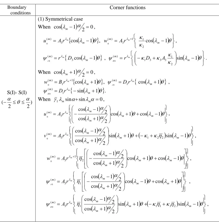
Table 1 Corner functions corresponding to symmetrical boundary conditions Boundary conditions Corner functions S(I)- S(I) ) 2 2 (−α ≤θ ≤α (1) Symmetrical case When

(

)

0 2 1 cosλ_m− α = ,

(

)

{

λ θ

}

λ 1 cos 3 ) ( 0 = m− m Ar m u ,

(

)

⎭ ⎬ ⎫ ⎩ ⎨ ⎧ − = + _{λ θ} κ κ λ 1 cos 2 1 1 3 ) ( 0 m m Ar m w ,

(

)

{

λ θ

}

ψ λ 1 cos 3 ) ( 0 = m− m _r m _D r ,

(

)

⎭ ⎬ ⎫ ⎩ ⎨ ⎧ − ⎟⎟ ⎠ ⎞ ⎜⎜ ⎝ ⎛ + − = λ θ κ κ κ κ ψ λ θ sin 1 2 1 3 3 3 1 ) ( 0 m m _r m _{D A .} When

(

)

0 2 1 cosλ_m+ α = ,

(

)

{

λ θ

}

λ 1 cos 1 1 ) ( 0 = + + m m Br m w , ψ 1 λ

{

cos

(

λ 1

)

θ

}

) ( 0 = m+ m m r Dr ,

(

)

{

λ θ

}

ψ λ θ 1 sin 1 ) ( 0 = − m+ m Dr m _.

When γ₁λ_msinα+sinλ_mα =0,

(

)

(

)

(

)

(

)

_⎪⎭⎪⎬ ⎫ ⎪⎩ ⎪ ⎨ ⎧ − + + ⎟ ⎟ ⎠ ⎞ ⎜ ⎜ ⎝ ⎛ + − − = _α λ θ λ θ λ α λ λ 1 cos 1 cos 2 1 cos 2 1 cos 3 ) ( 0 m m m m m Ar m u ,

(

)

(

)

(

) (

) (

)

_⎪⎭⎪⎬ ⎫ ⎪⎩ ⎪ ⎨ ⎧ − + − + + ⎟ ⎟ ⎠ ⎞ ⎜ ⎜ ⎝ ⎛ + − = _α λ θ κ κη λ θ λ α λ λ 1 sin 1 sin 2 1 cos 2 1 cos 2 2 1 3 ) ( 0 m m m m m Ar m v ,

(

)

(

)

(

)

(

)

_⎪⎭⎪⎬ ⎫ ⎪⎩ ⎪ ⎨ ⎧ ⎥ ⎥ ⎦ ⎤ ⎢ ⎢ ⎣ ⎡ − + + ⎟ ⎟ ⎠ ⎞ ⎜ ⎜ ⎝ ⎛ + − − = + _{λ θ λ θ} α λ α λ η λ 1 cos 1 cos 2 1 cos 2 1 cos 2 1 3 ) ( 0 m m m m m Ar m w ,

(

)

(

)

(

)

(

)

_⎪⎭⎪⎬ ⎫ ⎪⎩ ⎪ ⎨ ⎧ ⎥ ⎥ ⎦ ⎤ ⎢ ⎢ ⎣ ⎡ + + − ⎟ ⎟ ⎠ ⎞ ⎜ ⎜ ⎝ ⎛ + − − = _α λ θ λ θ λ α λ η ψ λ 1 cos 1 cos 2 1 cos 2 1 cos 1 3 ) ( 0 m m m m m m r Ar ,

(

)

(

)

(

) (

) (

)

_⎪⎭⎪⎬ ⎫ ⎪⎩ ⎪ ⎨ ⎧ − + − + + ⎟ ⎟ ⎠ ⎞ ⎜ ⎜ ⎝ ⎛ + − = _α λ θ κη κη λ θ λ α λ η ψ λ θ sin 1 sin 1 2 1 cos 2 1 cos 2 3 1 1 1 3 ) ( 0 m m m m m Ar m _,

Table 1 (Continued) S(I)- S(I) ) 2 2 (−α ≤θ ≤α where ] ) 4 ( ) 1 ( {[ 3 2 1 3 3 4 1 κ λm E C κ λm κ λm E η = − + − −

(

)

(

)

)]] 2 1 tan[ ] 2 1 cot[ [κ₁− λ_m− α λ_m+ α

(

)

(

)

)]]} 2 1 tan[ ] 2 1 cot[ ) 1 ( 1 [ 1 2 λ λ λ α λ α κ + − − − + + E m m m m )] )( ) 1 ( 1 ( [κ₂ − +κ₁ λ_m − −λ_m E₂ −C₁E₄ ,

(

)

(

)

]} 2 1 tan[ ] 2 1 cot[ { 1 1 2 2 _κ κ λ α λ α η = − _m− _m + . (2) Anti-symmetrical case When

(

)

0 2 1 sin λ_m − α = ,

(

)

{

λ θ

}

λ 1 sin 4 ) ( 0 = m− m Ar m u ,

(

)

⎭ ⎬ ⎫ ⎩ ⎨ ⎧ − = + _{λ θ} κ κ λ 1 sin 2 1 1 4 ) ( 0 m m Ar m w ,

(

)

{

λ θ

}

ψ λ 1 sin 4 ) ( 0 = m − m _r m _D r ,

(

)

⎭ ⎬ ⎫ ⎩ ⎨ ⎧ − ⎟⎟ ⎠ ⎞ ⎜⎜ ⎝ ⎛ − = λ θ κ κ κ κ ψ λ θ cos 1 2 1 4 3 4 1 ) ( 0 m m _r m _{D A} . When

(

)

0 2 1 sin λ_m + α = ,

(

)

{

λ θ

}

λ 1 sin 1 2 ) ( 0 = + + m m B r m w , ψ( ) ₂ λ

{

sin

(

λ 1

)

θ

}

0 = m+ m m r D r ,

(

)

{

λ θ

}

ψ λ θ 2 cos 1 ) ( 0 = m+ m D r m _.

When sinλ_mα−γ₁λ_msinα=0,

(

)

(

)

(

)

(

)

_⎪⎭⎪⎬ ⎫ ⎪⎩ ⎪ ⎨ ⎧ − + + ⎟ ⎟ ⎠ ⎞ ⎜ ⎜ ⎝ ⎛ + − − = _α λ θ λ θ λ α λ λ 1 sin 1 sin 2 1 sin 2 1 sin 4 ) ( 0 m m m m m Ar m u ,

(

)

(

)

(

) (

) (

)

_⎪⎭⎪⎬ ⎫ ⎪⎩ ⎪ ⎨ ⎧ − − + + ⎟ ⎟ ⎠ ⎞ ⎜ ⎜ ⎝ ⎛ + − − = _α λ θ κ κ η λ θ λ α λ λ 1 cos 1 cos 2 1 sin 2 1 sin 3 2 1 4 ) ( 0 m m m m m Ar m v ,

(

)

(

)

(

)

(

)

_⎪⎭⎪⎬ ⎫ ⎪⎩ ⎪ ⎨ ⎧ ⎥ ⎥ ⎦ ⎤ ⎢ ⎢ ⎣ ⎡ − + + ⎟ ⎟ ⎠ ⎞ ⎜ ⎜ ⎝ ⎛ + − − = + _{λ θ λ θ} α λ α λ η λ 1 sin 1 sin 2 1 sin 2 1 sin 3 1 4 ) ( 0 m m m m m Ar m w ,

Table 1(Continued)

(

)

(

)

(

)

(

)

_⎪⎭⎪⎬ ⎫ ⎪⎩ ⎪ ⎨ ⎧ ⎥ ⎥ ⎦ ⎤ ⎢ ⎢ ⎣ ⎡ − + + ⎟ ⎟ ⎠ ⎞ ⎜ ⎜ ⎝ ⎛ + − − = _α λ θ λ θ λ α λ η ψ λ 1 sin 1 sin 2 1 sin 2 1 sin 1 4 ) ( 0 m m m m m m r Ar ,

(

)

(

)

(

) (

) (

)

_⎪⎭⎪⎬ ⎫ ⎪⎩ ⎪ ⎨ ⎧ − − + + ⎟ ⎟ ⎠ ⎞ ⎜ ⎜ ⎝ ⎛ + − − = _α λ θ κη κη λ θ λ α λ η ψ λ θ cos 1 cos 1 2 1 sin 2 1 sin 3 3 1 1 1 4 ) ( 0 m m m m m Ar m _, where

(

)

(

)

]} 2 1 tan[ ] 2 1 cot[ { 1 1 2 3 _κ κ λ α λ α η = − _m + _m − . S(II)-S(II) ) 2 2 (−α ≤θ ≤α (1) Symmetrical case When

(

)

0 2 1 cos λ_m− α = and

(

)

0 2 1

cosλ_m+ α = , the corresponding corner functions are the same as those for S(I)_ S(I).

When γ1λmsinα+sinλmα =0 or λmsinα +sinλmα =0,

(

)

(

)

(

)

(

)

_⎪⎭⎪⎬ ⎫ ⎪⎩ ⎪ ⎨ ⎧ − + + ⎟ ⎟ ⎠ ⎞ ⎜ ⎜ ⎝ ⎛ + − − = λ θ λ θ α λ α λ λ 1 cos 1 cos 2 1 cos 2 1 cos 3 ) ( 0 m m m m m Ar m u ,

(

)

(

)

(

) (

) (

)

_⎪⎭⎪⎬ ⎫ ⎪⎩ ⎪ ⎨ ⎧ − + − + + ⎟ ⎟ ⎠ ⎞ ⎜ ⎜ ⎝ ⎛ + − = _α λ θ κ κ η λ θ λ α λ λ 1 sin 1 sin 2 1 cos 2 1 cos 2 2 1 3 ) ( 0 m m m m m Ar m v ,

(

)

(

)

(

)

(

)

_⎪⎭⎪⎬ ⎫ ⎪⎩ ⎪ ⎨ ⎧ ⎥ ⎥ ⎦ ⎤ ⎢ ⎢ ⎣ ⎡ − + + ⎟ ⎟ ⎠ ⎞ ⎜ ⎜ ⎝ ⎛ + − − = + _{λ θ λ θ} α λ α λ η λ 1 cos 1 cos 2 1 cos 2 1 cos 2 1 3 ) ( 0 m m m m m Ar m w ,

(

)

(

)

(

)

⎪⎩ ⎪ ⎨ ⎧ + − + − ⎟ ⎟ ⎠ ⎞ ⎜ ⎜ ⎝ ⎛ + − − − − = 3 4 1 1 5 ) ( ) 1 ( 2 1 cos 2 1 cos ) 1 ( 1 0 λ α η κ κ λ λ υ η α λ υ λ ψ λ m m m m m m m r Ar

(

λ 1

)

θ η cos

(

λ 1

) }

θ cos m− − 5 m + ,

(

)

(

)

(

)

⎪⎩ ⎪ ⎨ ⎧ + − + − ⎟ ⎟ ⎠ ⎞ ⎜ ⎜ ⎝ ⎛ + − − − = (1 ) 2 1 cos 2 1 cos ) 1 ( 1 1 1 4 3 ) ( 0 λ α η κ κ λ λ υ α λ υ λ ψ λ θ m m m m m m Ar m

(

λ 1

) (

θ κη κη

) (

sin λ 1

) }

θ sin m+ + 1 5 + 3 2 m − , where + + − + + − + + − + − − = ) ( ) 1 ( ) 1 ( ) 1 ( 4 1 2 2 4 2 1 4 1 2 1 4 1 2 1 1 4 E C E E C E C E E E C E E m m m λ λ η λ κ η ] ) 1 ( )[ 1 ( ) ( 2 1 4 2 1 3 2 1 3 4 2 _{E E C E} E C E λm κ κ κ λm η _{− + + + − − +} − ,