可程式化閘陣列之快速瑞立衰褪通道模擬器

國 立 交 通 大 學

電子工程學系 電子研究所碩士班

碩

士

論

文

可程式化閘陣列之快速瑞立衰褪通道模擬器

FPGA Channel Simulator of

Fast Rayleigh Fading Channel

研 究 生： 余子瀚

指導教授：魏哲和 博士

可程式化閘陣列之快速瑞立衰褪通道模擬器

研究生:余子瀚 指導教授:魏哲和 博士

國立交通大學電子工程系 電子研究所碩士班

摘要

在現今的無線通訊系統中，高速的資料傳輸速率以及可靠的通話品質一直是使用 者所最關切的。因此，設計一個系統，並且使其能在不同的環境下正常的操作便 成為工程師們的主要任務。為確保正常運作，系統必須經過不斷的模擬和測試。 然而，要在實際的環境裡做測試與模擬，卻是曠日費時，並且花費高昂。一個比 較實際的方法是使用通道模擬器去模擬真實世界裡會發生的各種不同的電波傳 遞特性。

我們在論文裡模擬的範例系統是以 OFDMA 為基礎的 IEEE 802.16a，特 別針對使用者在高速移動的環境下所做的快速瑞立 (Rayleigh) 衰褪通道模擬， 並且分析其複雜度，比較此通道模擬器所能提供之效能。

在這篇論文裡，我們以 Innovative Integration 公司的 Quixote 板來實現 通道模擬器。該板上裝置了一個德州儀器公司(Texas Instruments)出品的 TMS320 C6416 數位訊號處理器，以及一個智霖公司(Xilinx) 所出品的 Virtex II 可程式 化閘陣列(FPGA)。我們使用 FPGA 作為通道模擬器，並且討論三種不同的三角 函數產生方法在通道模擬器中的影響。此外，我們實現兩種單一快速 Rayleigh 衰 褪通道模擬器，其通道係數產生速度可超過每秒 100 百萬筆。最後，我們實現一 個六條快速 Rayleigh 衰褪通道模擬器，其每條通道每秒可產生 12.5 百萬筆通道 係數，可用來當作多重路徑通道或是用於多重輸出輸入(MIMO)系統之通道。

FPGA Channel Generator of

Fast Rayleigh Fading Channel

Student: Tzu-Han Yu Advisor: Dr. Che-Ho Wei

Department of Electronics Engineering

Institute of Electronics

National Chiao Tung University

Abstract

In today's wireless communication systems, the very issues which users care about the most are high data transmission rate and reliable quality. So, it becomes the most important task for engineers to make the system work in various environments.

In order to ensure the system performance, it requires simulations and tests. However, field testing for a wireless system is very costly and time consuming. A more practical way is to use a channel simulator to emulate the radio propagation characteristic.

In this thesis, we implement the channel generator with a DSP-FPGA embedded card-- "Quixote-III" produced by Innovative Integration. One DSP chip, TMS320C6416 of TI, and one FPGA chip, Virtex II of Xilinx, are placed on the card. We use FPGA to generate the channel coefficients. We also present three methods to implement the triangular function, which is also the most important component in a channel coefficient generator, and their influences on the speed of the simulator will be discussed and compared. Two single-fast Rayleigh fading channels are implemented, the yield rate of channel coefficient reaches 100 M data per second. Finally a 6-ray fast multipath fading channel is implemented, which can be used to simulate a multipath channel environment, and the channel coefficients yield rate reaches 12.5M per second each channel.

The wireless transmission system we simulate is IEEE 802.16a, focus on the fast Rayleigh fading channel for high mobility users. We shall analyze the complexity and make comparison.

致謝

首先，我要感謝我的指導教授魏哲和博士以及林大衛博士。由於他們的細心 指導，讓我在兩年的研究生生涯裡，漸漸從一個青澀的大學生，變成了現在能夠 獨立思考，並擁有解決問題能力的我。同時在寫作論文的過程中，兩位老師不時 的指正我的錯誤，並且指引我往正確的學問之道走去，使我不至於失去方向，更 扎實了我做研究的基礎。 實驗室裡的唐之璇學姐，林郁男學長，王士豪學長，吳俊榮學長以及鍾翼州 學長也常在我碰上困難的時候給予我指點，讓我不會徬徨無助。另外同級的曾建 統同學，李明哲同學，陳盈縈同學，林筱晴同學，蔣宗書同學，黃名彥同學，莊 孝強同學，陳俊安同學以及蘇子良同學也都會相互砥礪，研討功課，並且陪我走 過這令人懷念的兩年。 最後，我要感謝我的父母親以及我的妹妹，感謝他們一直都在我背後支持 我，給予我親情上的支持，讓我可以心無旁鹜的完成我的學業。 在此，僅將此篇論文獻給所有幫助過我的人。

Contents

摘要

………

i

Abstract………...

ii

致謝

………..

iv

Contents………..v

List of Figures………...vii

List of Tables………..ix

Chapter 1 Introduction………...1

Chapter 2 BWA Communication Standards……...3

2.1 Overview of BWA Communication Standards….………..3

2.2 Overview of OFDM and OFDMA……….4

2.2.1 OFDM………...5

2.2.2 OFDMA………..10

2.3 Physical Layer of IEEE 802.16a OFDMA Mode………10

2.3.1 Carrier Allocation for Downlink……….11

2.3.2 Carrier Allocation for Uplink………..14

2.3.3 OFDMA Frame Structure for TDD……….15

Chapter 3 System Overview…..………...18

3.1 Channel Parameters……….……….19

3.2 Channel model……….……….21

3.2.1 Delay profile………24

3.2.2 Channel Coefficients ………...26

3.3 Bottleneck for the system when operating at high speed……….31

Chapter 4 Hardware Implementation…………...34

4.1.1 DSP Chip Introduction……….36

4.1.2 Xilinx FPGA Chip ………...40

4.1.3 Data Transmission Mechanism………41

4.2 Fundamental Functions for Channel Coefficients……….……42

4.2.1 Triangular Function Generator……….……42

4.2.2 Pseudo Random Number Generator……….………50

4.3 Channel Simulator………....……….52

4.3.1 Single-ray Channel Simulator………..……....53

4.3.2 Multipath Channel Simulator………..……...…61

4.4 Complexity and Performance………..….….65

4.4.1 Analyses of Complexity………...…65

4.4.2 Realistic Performance ………...……66

Chapter 5 Conclusion………..67

Reference……….68

List of Figures

Fig 2.1: The CP is a short copy of the last part of the OFDM symbol……….6

Fig 2.2: A basic view of a digital baseband OFDM system……….6

Fig 2.3: OFDM system as a set of parallel channels………9

Fig 2.4.: OFDMA frequency description (3 Subchannel example)……….11

Fig 2.5: Carrier allocation in The OFDMA DL………..13

Fig 2.6: Carrier allocation in the OFDMA UL………...15

Fig 2.7: Time plan for one TDD time frame………...17

Fig 3.1: The system block diagram……….18

Fig 3.2: Main task of Channel simulator……….19

Fig 3.3: An OFDMA symbol in our system………21

Fig 3.4: Types of multipath fading………...23

Fig 3.5: Doppler power spectrum……….27

Fig3.6: Autocorrelation of X_c

( )

t ………...30

Fig3.7: Autocorrelation of X_s

( )

t ………...30

Fig 3.8: Crosscorrelation ofX_c

( )

t andX_s

( )

t ……….30

Fig 3.9: Autocorrelation of X(t)………...30

Fig 4.1: Quixote-III………..34

Fig 4.2: Block diagram of Quixote-III……….35

Fig 4.3: Block diagram of TMS320C6416………..36

Fig 4.4: C64X CPU structure……….………..37

Fig 4.5: General Slice Diagram………40

Fig 4.8: Trigonometric Fan………..46

Fig 4.9: The coordinate view………..….47

Fig 4.10: Example of CORDIC………...47

Fig 4.11: The generation of a pseudo random binary sequence………..50

Fig 4.12: Correlation function of a Pseudo Random sequence………...51

Fig 4.13: The demonstration of Jakes model with CORDIC………..54

Fig 4.14: The demonstration of Jakes model with LUTs………54

Fig 4.15: The demonstration of Jakes model with Taylor series……….55

Fig 4.16: The demonstration of Jakes model with LUTs (as comparison)…………..55

Fig 4.17: The demonstration of Xiao model with LUTs……….58

Fig 4.18: The demonstration of Xiao model with CORDIC………...58

Fig 4.19 Autocorrelation of Xc

( )

t ………...60

Fig 4.20: Autocorrelation of Xs

( )

t ………...60

Fig 4.21: Crosscorrelation of Xs

( )

t andXc

( )

t ……….61

Fig 4.22: Real part autocorrelation of X(t)………..61

Fig 4.23: The demonstration of Xiao model with CORDIC………...63

List of Tables

Table 2.1: OFDMA carrier allocation for downlink……….12

Table 2.2: OFDMA carrier allocation for Uplink……….14

Table 3.1: OFDMA carrier allocation for Downlink………20

Table 3.2: Channel Parameters and OFDMA Symbol Parameters………...21

Table 3.3: Percentage of time the particular channel………...25

Table 3.4: Indoor Office Test Environment Tapped-Delay-Line Parameters………..25

Table 3.5: Outdoor to indoor and Pedestrian Test Environment Parameters………...25

Table 3.6: Vehicular test Environment Tapped-Delay-Line Parameters………..26

Table 4.1: C64x CPU Function units and Operation performed………..38

Table 4.2: C64X CPU Function units and Operation performed……….39

Table 4.3: Comparison of LUTs………...44

Table 4.4: The accumulating angles……….46

Table 4.5: Comparison of Triangular Functions………...49

Table 4.6: Comparison of Triangular Algorithms………49

Table 4.8: Feedback connections for generation of pseudo random sequence………51

Table 4.9: The random seeds for each Pseudo random generator………52

Table 4.10: The FPGA implementation results of PN generator………..52

Table 4.11: Comparison of Jakes’ model with different triangular Algos………56

Table 4.12: Initial phase of ψ_n………....57

Table 4.13: Comparison of Xiao model with different triangular Algos………..59

Table 4.14: Simulation parameters………...62

Table 4.15: Simulation results………..64

Chapter 1

Introduction

Recent years, with the rapid progress of technology, people start to demand for better quality of life. Among these needs, communication between people is one of the most challenging ones. From the wire-line telecommunication in the 19th century to the latest wireless communication systems in the 21st century, the design constraints and implementation difficulties are getting higher and higher. People ask for high data transmission rate to deliver and receive multimedia information, high mobility support for them to be able to use the service while traveling at high speed.

However, to design and implement such a wireless system requires a lot of simulations and tests. But, field testing for a wireless system is very costly and time consuming, and even though we actually do the field test, the wireless environment changes over time, place and the speed which the subscriber is moving. A better way is to use a channel simulator to emulate the radio propagation characteristic, and simulate the whole system performance.

In this thesis, we will design and implement a channel simulator for a wireless communication system based on OFDM, especially focus on high speed moving environment.

The channel simulator will be implemented on a FPGA chip. We use a

DSP-FPGA embedded card as our hardware platform, which contains a digital signal

processor (DSP) and a field programmable gate array (FPGA). (Further details will be introduced in Chapter 4.) We implement two single-fast Rayleigh fading channels and a 6-ray fast Rayleigh fading channel, respectively. We also discuss the triangular function algorithms that influence the performance of channel simulators.

The rest of the thesis will be organized as followed: In Chapter 2, we will introduce the IEEE 802.16a specification. And Chapter 3 will introduce our system to be implemented. Then, the hardware information and simulator structure will be discussed in Chapter 4. In this chapter, we also present three methods to implement

the triangular function, which is also the most important component in a channel coefficient generator, and their influences on the speed of the simulator will be discussed and compared. The final results and conclusions are given in Chapter 5.

Chapter 2

BWA Communication Standards

2.1 Overview of BWA Communication Standards

BWA (Broadband wireless access) is the most challenging segment of the wireless

revolution since it has to demonstrate a viable alternative to the cable modem and

DSL (Digital Subscriber Lines) technologies that are strongly entrenched in the last

mile access environment. It is also the best way to meet the rising need of rapid multimedia information nowadays [1]. Wireless transmission standards, such as European DAB (digital audio broadcasting) standard [10], ETSI (European

Telecommunications Standard Institute) HyperLan/2 [11], DVB-T [12], IEEE

802.11b [13], IEEE 802.11g [14], IEEE 802.11a [15], and IEEE 802.16a [4] can all

be specified as BWA communication standards. And we take IEEE 802.16a as our example in this thesis.

IEEE 802.16[3] as a standard which specifies the WirelessMan Air Interface for

wireless metropolitan networks. It was the first step for IEEE to adapt BWA as a standard specification. IEEE 802.16 addresses the “first mile/last mile” connection in wireless metropolitan are networks and focuses on the efficient use of bandwidth between 10 and 66 GHz and defines a medium access control (MAC) layer that supports multiple physical layer specifications customized for frequency band of use [2].

IEEE 802.16a [4] specification enhances the medium access control layer and its

operating frequency is between 2 to 11 GHz, mainly used as a fixed point (non-moving) broadband wireless transmission scheme. There are three modes in 802.16a for operators to chose, they are: single carrier mode, OFDM mode and

OFDMA mode (OFDM and OFDMA will be further introduced latter.). And we will

take OFDMA as our consideration.

means that the specification may not be working when users are moving at high speed. So, in this thesis, we try to implement a channel simulator which simulates the channel while users are moving at high speed with a large Doppler shift (up to 2000 Hz) for checking how the mobility rate can 802.16a supports. And this channel simulator can be also used in other systems. For instance, IEEE 802.16’s Task Group E is now working on modifying 802.16a to 802.16e which can support high mobility usage. Another group under IEEE PAR 802.20 is also seeking for a novel BWA scheme to support high mobility, too. This channel simulator could be used in these systems as well.

2.2 Overview of OFDM and OFDMA [5]

OFDM (Orthogonal Frequency Division Multiplexing) is usually viewed as a

transmission scheme which can be applied in the wireless environment and in the wireline communication system, also.

The history of OFDM could be traced back to the 60’s, when Chang published his paper on the synthesis of bandlimited signals for multichannel transmission [6]. Chang presented a scheme of transmitting signals simultaneously through a linear bandlimited channel without ICI (interchannel interference) and ISI (intersymbol

interference). Later on, Salzberg performed an analysis of the performance [7], where

he concluded that “the strategy of design an efficient parallel system should concentrate more on reducing crosstalk between adjacent channel than on perfecting the individual channels themselves, since the distortions due to crosstalk tend to dominate”.

In 1971, Weinstein and Ebert made a major contribution to OFDM, they used

DFT (Discrete Fourier Transform) to perform baseband signal modulation and

demodulation [8]. They also added a guard space between the symbols and raised-cosine windowing in the time domain to avoid ISI and ICI. Another important

contribution was due to Peled and Ruiz in 1980 [9]. They came up with the idea of

CP (cyclic prefix) solving the orthogonality problem. Instead of using an empty guard

space, they filled the guard space with cyclic extension of the OFDM symbol. By doing this, when the OFDM signals are transmitted through the channel, effectively simulates a channel performing cyclic convolution, and implies orthogonality over dispersive channels when CP is longer than the impulse response of the channel.

Recent years, another OFDM based technique—OFDMA (Orthogonal Frequency

Division Multiple Access) has been modified from OFDM to get a better bandwidth

share idea for multiple users. In OFDMA, the carriers are divided into groups which are called subchannels for multiple users to use within one single OFDMA symbol while in OFDM, one user is allowed only.

OFDM and OFDMA are now widely used in many wireless or wireline

transmission standards, such as European DAB (digital audio broadcasting) standard [10], ETSI (European Telecommunications Standard Institute) HyperLan/2[11],

DVB-T [12], IEEE 802.11b [13], IEEE 802.11g [14], IEEE 802.11a [15], and IEEE 802.16a.

2.2.1 OFDM

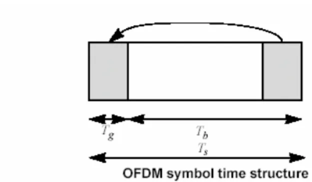
The basic idea of OFDM is to divide the available spectrum into several subchannels. By making all subchannels narrowband, they experience flat fading, which makes equalization very simple. To obtain a high spectral efficiency the frequency response of the subchannels are overlapping and orthogonal. The orthogonality can be maintained, even though the signal passes through a time-dispersive channel, by introducing a CP (cyclic prefix). An OFDM symbol is shown in Figure 2.1

Fig 2.1: The CP is a short copy of the last part of the OFDM symbol

where Tg represents the time length of CP, which is a short copy of the last part of the OFDM symbol, and Tb represents the data interval. By introducing CP, we can avoid the occurrence of ISI and ICI at the cost of losses in SNR (Signal to Noise Ratio) and throughput will be introduced.

A basic OFDM system diagram is given in Figure 2.2

Fig 2.2: A basic view of a digital baseband OFDM system

From Fig 2.2, we can see how an OFDM symbol is formed, transmitted and received. First of all, binary data from the source are mapped (may be in BPSK,

QAM, 16-QAM, or 64-QAM form), then separated from serial sequence to parallel

sequence. After that, we insert pilot carriers which will be used when doing channel estimation, then, perform IDFT (Inverse Discrete Fourier Transform). Finally, we add

CP, an OFDM symbol is formed. Through the channel, the signal will be transmitted

to the receiver and demodulated with the counter steps as what had been done in the transmitter end. Thus, an OFDM transmission process is completed.

system. However, in most of the case, we implement such a system in the discrete-time form. But, we still like to introduce OFDM from the viewpoint of continuous-time OFDM system.

Consider an OFDM system consisting of N subcarriers with a bandwidth of W Hz. The symbol time is T seconds long, composed of Ts and Tg, where Ts= N/W seconds which represents the real data interval, and Tg seconds is the time interval of CP. The transmitted signal for the kth subcarrier could be expressed as

where T=Ts +Tg . Note that g_k

( )

t =g_k

(

t+T_s

)

when t is within the guard interval [0, Tg]. We also notice that g_k

( )

t is a rectangular pulse modulated by the carrier

frequency KW

N. The transmitted baseband signal s(t) for the OFDM symbol l can be

obtained by summing all modulated subchannel signals as

( )

(

)

1 , 0 N l k l k k S t x g t lT − = =

∑

− (2.2)

where x_0,l,x_1,l,...,x_n−1,l are complex numbers from a set of signal constellation points, which represent the transmitted data. From (2.1) and (2.2), we can see that

( )

0 l

s t = for t∉

[

lT l, ( +1)T

]

. This way, the baseband signal s(t) can be expressed as:

( )

( )

1 ,

(

)

0 N l k l k t t k s t s t x g t lT ∞ ∞ − =−∞ =−∞ = =

∑

=

∑ ∑

− (2.3)

We assume that the impulse response h

( )

τ;t is shorter than the length of CP, then, the received signalr t

( )

will be

( ) (

*

)( ) ( )

=

( ) (

)

( )

0 ; g T h t s t−τ τd +n t

∫

, (2.4)

where n(t) is additive, white, and complex Gaussian noise.

The OFDM receiver consists of a filter bank, matched to the last part [Tg, T] of the transmitted waveformg_k

( )

t , that is,

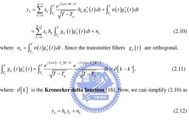
It means that CP is removed in the received signal, and the signal is clean without ISI. Now we can omit the time index l when calculating the sampled output at the kth matched filter. Through (2.3), (2.4) and (2.5), we find that

(

)( )

| k k t T y = ∗τ u t ₌ = r t u T

( ) (

k t dt

)

∞ −∞ −

∫

=

(

( ) (

)

( )

)

( )

0 ; g g T T k T h τ t s t τ τd n t g t dt ∗ − +

∫ ∫

=

( )

(

)

( )

( ) ( )

1 ' ' 0 ' 0 ; g g N T Tg T k k k k T T k h τ t x g t τ dt g t dt n t g t dt − ∗ ∗ = ⎛ ⎡ ₋ ⎤ ⎞ ₊ ⎜ ⎢_⎣ ⎥_⎦ ⎟ ⎝

∑

⎠

∫ ∫

∫

(2.6)

Assuming that the channel response is static over one OFDM symbol interval and is denoted ash

( )

τ , then

(

( ) (

)

)

( )

( ) ( )

1 ' ₀ ' ' 0 g g g N _{T T T} k k _T k k _T k k y x h τ g t τ g t dt n t g t dt − ∗ ∗ = =

∑ ∫ ∫

− +

_∫

(2.7) From (2.7), we can see that T_g < < and t T 0< <τ T, then 0< − <t τ T . Therefore, by substituting (2.1) to (2.7), the inner integral of (2.7) becomes

( ) (

)

( )

( ) 2 ' / ' 0 0 g g g j k t T w n T T k g e h g t d h d T T π τ τ −τ τ = τ − − τ −

∫

∫

( )

( )

2 ' / 2 ' / , g g j k t T W N T j k W N e h e d π π τ τ τ − − = −

∫

Tg < < (2.8) t T

Furthermore, the integral in (2.8) is the sampled frequency response of the channel at the kth subcarrier frequency f=k’W/N:

( )

2 ' / ' ' ₀ , g T j k W N k W h H K h e d N π τ τ − τ ⎛ ⎞ = _{⎜ ⎟}= ⎝ ⎠

∫

(2.9)

where H(f) is the Fourier transform of h

( )

τ . The output from the receiver filter bank can be rewritten as

( )

( ) ( )

2 ' / 1 ' ' ' 0 g g j k W N N _{T T} k k k k k T T k _g e y x h g t dt n t g t dt T T π τ − ∗ ∗ = = + −

∑ ∫

∫

( ) ( )

1 ' ' ' ' 0 g N _T k k _T k k k k x h g t g t dt n − ∗ = =

∑

∫

+ (2.10) where

( ) ( )

g T k k T

n =

∫

n t g∗ t dt. Since the transmitter filters gk

( )

t are orthogonal,

( ) ( )

2 '( ) / 2 ( ) /

[

]

' ' g g g g j k t T W N j k t T W N T T k k T T g g e e g t g t dt k k T T T T π π δ − − − ∗ _{= = −} − −

∫

∫

, (2.11)

where δ

[ ]

k is the Kronecker delta function [16]. Now, we can simplify (2.10) as

y_k =h x_{k k} + (2.12) n_k

where n_k is additive white Gaussian noise.

By re-introducing time index l, we may now view the OFDM system as a set of parallel channels, just as Figure 2.3.

2.2.2 OFDMA

The basic idea of OFDMA is an OFDM based frequency division multiple access. The main structure and transmission technique are very alike. But, in OFDMA, the carriers are divided into groups which are called subchannels, and the number of subcarriers for each subchannel depends on the system design. Users are allowed to use one or more subchannels on their demand, which means that OFDMA support multiple users within one OFDMA symbol. While in OFDM structure, only one single user is allowed. So, by doing subchannelizing the symbol in the frequency domain, the bandwidth can be allocated dynamically and efficiently. That is the major difference between OFDM and OFDMA.

Due to the large variance of transmission path loss in the wireless environment, the intercell interference is one of the impairments in wireless communication. In OFDMA system, the subchannels can be composed from several distinct permutations of subcarrirers, and this enables significant reduction in the intercell interference, if the system is not fully loaded. This is another advantage for OFDMA.

As what had been described above, OFDMA is more complex than OFDM since it supports multiple users, and introduces the idea of subchannels, which make it even harder for implementation. We make a further description in the next part, how IEEE 802.16a formulate the OFDMA structure and make it work perfectly.

2.3 Physical Layer of IEEE 802.16a OFDMA Mode

In IEEE 802.16 specification, it formulates wide range of aspects in the whole system, but we only underline some of the PHY (Physical Layer) for the OFDMA mode in this thesis, since PHY concerns the channel simulator the most. Other detailed information could be found in the 802.16a specification [4].

2.3.1 Carrier Allocation for Downlink

The FFT size in the 802.16a OFDMA mode for downlink is 2048, which means that there are 2048 subcarriers within a channel. Among these subcarriers, they are mainly divided into tree groups: data carriers used to carry the information, pilot carriers used for channel response estimation and various synchronization purposes, and null carriers, including guard bands and DC carrier, carrying no useful information at all. The frequency description is shown in Figure 2.4.

Fig. 2.4: OFDMA frequency description (3 subchannel example)

As we can see in Figure 2.4, among those 2048 subcarriers, there are 1702 used subcarriers, composed of 1536 data carriers and 166 pilot carriers. The rest 346 subcarriers are unused subcarriers as the guard band distributed on the edges of the symbol, and one DC carrier right in the middle of the OFDMA symbol. In, IEEE 802.16a those 1702 used subcarriers are divided into 32 subchannels, each subchaneel consists of 48 data carriers and 2 fixed pilot carriers and 3 variable location pilot carriers. The pilot location changing rule follows some permutation formula which will be described latter. The carrier allocation for OFDMA in 802.16a is listed in Table 2.1.

Table 2.1: OFDMA carrier allocation for downlink

As what had mentioned above, there are variable location pilot carriers and fixed location pilot carriers in the downlink OFDMA symbol. The carrier indices of the fixed location pilots never change. The variable location pilots shift their location every symbol, repeating every 4 symbols, according to the formula:

varLocPilot=3L+12P_k L∈0,1, 2, 3 P_k∈

{

0,1, 2...141

}

(2.13) wherevar LocPilot is the carrier index of variable location pilot . The detailed illustration is given in Figure 2.5

After mapping the pilot carriers, the remainders of the used carriers are the data subchannels. Note that since the variable location pilots change location in each symbol, repeating every fourth symbol, the locations of the carriers in the data shall change also.

Fig 2.5: Carrier allocation in The OFDMA DL

The exact partitioning into subchennels is done according to (2.14) [1], called a permutation formula.

( )

, subchannels

{

s mod(Nsubchannels) cell

(

1 /

)

subchannels

}

mod(Nsubchannels)

carrier n s =N • +n p _⎣⎡n _⎦⎤+ID •ceil⎡_⎣ n+ N ⎤_⎦

(2.14) where

( )

,

carrier n s is the carrier index of carrier n in subchannels

s is the index number of a subchannel, from the set

[

0,1...Nsubchannels −1

]

,

n is the carrier-in-subchannel index from the set

[

0,1...Nsubcarries−1

]

, subchannels

N is the number of subchannels,

[ ]

s

p j is the series obtained by rotating{PermutationBase}cyclically to the left s times,

[ ]

cell

ID is a positive integer assigned by MAC to identify this particular BS,

( )

modk

X is the remainder of quotient X/k (which is almost k-1),

2.3.2 Carrier Allocation for Uplink

In uplink OFDMA symbol, the FFT size remains 2048. The subcarriers are also divided into data carriers , pilot carriers and unused carriers, just as in downlink. The allocation of subcarriers is slightly different from downlink. There are 1696 used subcarriers, composed of 1536 data carriers and 160 pilot carriers. The rest 352 subcarriers are unused subcarriers as the guard band distributed on the edges of the symbol, and one DC carrier right in the middle of the OFDMA symbol. In IEEE 802.16a, those1696 used subcarriers are divided into 32 subchannels, each subchaneel consists of 48 data carriers and 1 fixed pilot carriers and 4 variable location pilot carriers. The carrier allocation for OFDMA in 802.16a is listed in Table 2.2.

The fix location pilot location is always at 26 in the subchannel. The variable location pilots change locations in each symbol, repeating every 13 symbols, according to L_k = 0, 2, 4, 6, 8, 10, 12, 1, 3, 5, 7, 9, 11, where k=0 to 12. For k=0 the

variable location pilots are placed at 0, 13, 27, 40. For other k values, the locations change by adding L_k to the index. The subchanel division scheme in uplink also obeys (2.14). And the detailed carrier illustration is given in Figure 2.6.

Fig 2.6: Carrier allocation in the OFDMA Uplink

2.3.3 OFDMA Frame Structure for TDD

IEEE 802.16a is designed to operate in the frequency band between 2 to 11GHz. If the system is operating in licensed bands, the duplexing method shall be either FDD

(Frequency Division Duplexing) or TDD (Time Division Duplexing). But when the system is operating in frequency-exempt band, the duplexing method must be TDD. We consider the TDD mode in this thesis. For the traffics of the downlink users and the uplink users are usually quite asymmetric. TDD permits efficient allocating the available resources, since uplink transmissions are usually much less then the

downlink transmissions.

Figure 2.7 is the frame structure of TDD OFDMA. In order to fit the FEC

(Forward Error Coding) block, each burst transmission consists of multiples of three

OFDMA symbols. In each frame, one DL subframe and one UL subframe are contained. Each subframe contains numbers of bursts. In each frame, the TTG (Tx/Rx

transition gap) and Rx/Tx transition gap (RTG) shall be inserted between the downlink and uplink at the end of each frame respectively to allow BS (Base Station) to turn around. TTG and RTG shall be at least 5us and integer multiple of the PS in duration, and start on a PS boundary. After the TTG, the BS receiver shall look for the first symbols of a UL burst. After RTG, the SS (Subscriber Station) receiver shall look for the first symbols of QPSK modulated data in the DL burst. The duration of a frame is limited from 2 ms to 20 ms and is specified by the frame duration code.

In the beginning of the frame, there are some important information for downlink and uplink. As we know, the control messages and the system parameters are very important for the BS and the SS. So, the first burst contains the parameters such as modulation type, forward error correction type, preamble length, guard time, etc. The first FEC block of each frame is the DL_Frame_Prefix. It contains the parameters of

FCH (Frame Control Header) which includes DL-MAPs and UL-MAPs and other information. DL-Maps and UL-Maps messages define the access to the downlink and uplink information, including the burst profiles and allocation in the subchannel and time axes of the bursts.

After a short TTG, all pilot symbols called preamble will be inserted by the SS to help the channels estimation process in the receiver, since for uplink users, the subcarriers spread out in the whole channel, it will be very difficult to BS to make a precise channel estimation with only 5 pilots in a subchannel.

Fig 2.7: Time plan for one TDD time frame

Above, we briefly introduce the technique background ,operating environment , physical layer parameters and structures of IEEE 802.16a in OFDMA mode, other detailed information, such as MAC (Medium Access Control) layer, channel coding, interleaving scheme in PHY, synchronization problems, channels estimation difficulties, etc. are not discussed in this thesis, since the carrier allocation and frame structure concern channel simulator the most. Those skipped information could be found in IEEE 802.16a [4].

Chapter 3

System Overview

After the brief introduction to IEEE 802.16a in OFDMA mode, we would like to introduce our system which follows the specification.

Fig 3.1: The system block diagram.

Figure 3.1 shows a wireless transmission system in detail. The channel simulator that we are going to implement is shaded in the diagram for the simulation. The main task for a channel simulator can be expressed in Figure 3.2.

The channel simulator generates channel coefficients following some specific channel model, then convolutes the channel coefficients with the transmitted signals s(t) from Tx, and then adds the noise item. Finally, it sends the resulting signals y(t) to the Rx end. We can also express it by an equation:

( ) ( ) ( ) ( )

where h t

( )

denotes the channel coefficients which is our main task for the channel simulator, n t

( )

is the noise item, and“∗” represents the convolution operation in time domain.

Fig 3.2: Main task of Channel simulator

In order to generate the proper channel coefficients to simulate the electro-magnetic wave propagation, we have to clearly understand the system channel parameters and choose a suitable channel model for the simulator.

3.1 Channel Parameters

IEEE 802.16a supports the wireless access operating at frequencies 2-11 GHz. In this thesis, we assume that our system operates at 2 GHz band. From the Annex B in

IEEE 802.16a, our system channel parameters are defined by the specification, which is shown in Table 3.1.

In Table 3.1, we can find that there are two bandwidths for us to choose, and we take 10 MHz in our study. The ratio of CP time to the useful time is supported as 1/32,

1/16, 1/8 and 1/4, and we pick 1/8. The number of FFT (Fast Fourier Transform) and the useful time Tb for OFDMA are defined as 2048 and 179.2 us, so the CP time, Tg, is 22.4 us. The sampling frequency is defined as (BW • 8/7), where BW is the bandwidth. The OFDMA symbol parameters and system channel parameters are now all determined and listed in Table 3.2. And Figure 3.3 shows a schematic picture of an

OFDMA symbol in our system.

Table 3.l: OFDMA Channelization Parameters For License-exempt Bands [3].

Table 3.2: Channel Parameters and OFDMA Symbol Parameters

Fig 3.3: An OFDMA symbol in our system

3.2 Channel model[18]

After the channel parameters are determined, we now have to pick a suitable channel model for our system simulation.

Modeling the radio channel has been considered as one of the most difficult parts in wireless communication system design. The transmission paths between transmitter and receiver may vary with different terrains, buildings, the speed that mobile terminals move, the season factors, even the wind speed. [17]

The radio wave propagation effects are mainly divided into two parts. One is shadow fading, and the other is multipath fading. Shadow fading basically involves the electro-magnetic wave reflection, diffraction, scattering and attenuation, while small multipath fading involves multipath effects essentially. In most of the cases, multipath fading is more critical than large-scale fading. Multipath effects generally affect greatly the on the channel response estimation and synchronization of the system. Thus, we consider the multipath fading in the simulation only.

With multipath fading effects, the signal strength may changes within a short period of time, and the varying Doppler shifts on those different paths may undergo the random frequency modulation.

The cause of multipath fading is due to the interference between two or more versions of the transmitted signal which arrive at the receiver at the different time. Many factors influence the multipath fading, including multipath propagation, speed of the mobile, surrounding constructions, and transmission bandwidth as well. The constructive and destructive combinations cause fluctuations in the signal strength.

Moreover, the relative motion between the base station and the mobile terminal results in random frequency modulation due to different Doppler shifts on each if the multipath components. Doppler shifts may be positive or negative depending on whether the mobile receiver is moving toward or away from the base station. The Doppler shift f_d is given by

f_d=v cosφ

λ (Hz) (3. 2)

where v is the mobile speed (in meter/second), λ is the wavelength of the

transmitted signal (in meter), and φ is the spatial angle between the direction of the mobile terminal and the direction of arrival of the wave.

There are also different types of multipath fading. Depending on the relation between the signal parameters (such as bandwidth, symbol period, etc.) and channel parameters (such as R.M.S delay spread and Doppler spread), different transmitted signals will undergo different types of fading. The time dispersion and frequency dispersion mechanisms lead multipath fading to four types. Figure 3.4 shows a tree of the four types of fading.

In flat fading, the multipath structure of the channel is such that the spectral characteristics of the transmitted signal are preserved at the receiver. However the strength of the received signals changes with time. On the other hand, in frequency

greater than the reciprocal bandwidth of the transmitted waveform. Thus, the channel induces ISI, and signal will distort.

Fig 3.4: Types of multipath fading [37]

Depending on how rapidly the transmitted baseband signal changes as compared to the rate of change of the channel, a channel may be classified either as a fast or slow fading channel. In fast fading channel, the channel impulse response changes rapidly within the symbol duration, while in slow fading channel, the channel impulse response changes at a rate which is much slower than the transmitted signal.

Another important factor in the channel model is the noise item. There are untold random noise sources from the surrounding in an actual environment .Those noise sources may be from the atmosphere, the sun, cosmos, or manmade sources. We usually model the noise as additive white Gaussian noise (AWGN) with zero mean and constant variance.

A channel model consists of AWGN, channel multipath delay spread, and channel coefficients, and when all of them are determined, we can start to simulate our

channel model.

3.2.1 Delay profile

A delay profile contains the information of channel multipath number, average power of each path ,etc. The delay profile changes over the terrestrial constraints and the moving speed. ETSI (European Telecommunications Standard Institute) provides us a suitable delay profile for our channel model in ESTI TR 101112V.3.2.0 [19]. For each terrestrial test environment, a channel impulse response model based on a tapped-delay line model is given. The model is characterized by the number of taps, the time delay relative to the first tap, the average power relative to the strongest tap, and the Doppler spectrum of each tap. A majority of the time, r.m.s delay spreads are relatively small, but occasionally, there are “worst case” multipath characteristics that lead to much larger r.m.s delay spreads. Measurements in outdoor environments show that the r.m.s delay spred can vary over an oder magnitude, within the same environment. Although large delay spreads occur relatively infrequently, they can have a major impact on the system performance. To accurately evaluate the relative performance of candidate RTTs (Run Trip Time), it is desirable to model the variability of delay spread as well as the “worst case” locations where delay spread is relatively large.

As this delay spread variability cannot be captured using a single tapped delay line, up to two multipath channels are defined for three environments. Within each environment, channel A is the low delay spread case that occurs frequently, channel B is the median delay spread case that also happens frequently. Each of these two channels is expected to be encountered for some percentage of tine in a given test environment. Table 3.3 gives the percentage of time the particular channel may be encountered.

Table 3.3: Percentage of time the particular channel [19]

The following tables describe the tapped-delay-line parameters for each of the terrestrial environments. For each tap of the channels three parameters are given: the time delay relative to the first tap, the average power relative to the strongest tap, and Doppler spectrum of each tap. A small variation,±3%, in the relative time delay is allowed so that the channel sampling rate can be made to match some multiple of the link simulation sample rate[19].

Table 3.4: Indoor Office Test Environment Tapped-Delay-Line Parameters [19]

Table 3.6: Vehicular test Environment Tapped-Delay-Line Parameters [19]

3.2.2 Channel Coefficient

In 1968, Clarke developed a model where statistical characteristics of the electro-magnetic fields of the received signal at the mobile are deduced from scattering [20].

( )

c

( )

s

( )

g t =g t + jg t (3. 3) where

( )

0

(

)

1 cos 2 cos N c n d n n n g t E C πf t α φ = =

∑

+ (3. 4) and

( )

0

(

)

1 sin 2 cos N s n d n n n g t E C π f t α φ = =

∑

+ (3. 5) d

f is the Doppler shift as expressed in (3.2), N is the path number, E is the real ₀

amplitude of local average E-field, α_n,φ_n are the random phases distributed from 0

to 2π , C is a random variable representing the amplitude of individual wave, and _n

2 1 1 N n n C = =

∑

(3. 6) Latter on, Gans developed a spectrum analysis for Clarke model in 1972 [21], the power spectral density can be expressed as

( )

(

)

2

( ) ( )

( ) ( )

2 m c P S f p G p G f f f α α α α = ⎡_⎣ + − − ⎤_⎦ − − (3. 7)

where f is the maximum Doppler frequency, _m p

( )

α α is the fraction of the total d

incoming power within dα of the angle α , G

( )

α is the antenna gain, and P is

the average received power with respect to an isotropic antenna. The Doppler power spectrum S f

( )

has a U shape as shown in Fig. 3.5.

Fig 3.5: Doppler power spectrum [37]

With Doppler power spectrum, we can generate the fading channel coefficients. However, to generate the channel coefficients which follow the Clarke model takes three random number generators, it makes implementing random number generator itself a difficult task. In 1974, Jakes came up with a simplified model [22].

( )

c

( )

s

( )

u t =u t +u t (3. 8) where

( )

( )

0 2 cos M c n n n u t a w t N = =

∑

(3. 9)

( )

( )

0 2 cos M s n n n u t b w t N = =

∑

(3.10) and

This model has been used for decades for its simple structure. As we can see, there is no random variable needed, and this reduces the complexity of implementation.

However, Jakes model is a deterministic model, which means that if the parameters are given, the model will generate the same coefficients. While simulating multiple uncorrelated channels, Jakes model must be modified. Moreover, the statistical behaviors of Jakes model leave much space to improve.

From the Clarke model in (3. 3) to (3. 5), we find that the second order statistical properties are:

( )

( ) (

)

(

)

( )

(

)

( )

( )

( )

( ) (

)

(

)

0 0 0 0 0 2 c c s s c s s c g g c c d g g d g g g g gg d R E g t g t J w R J w R R R E g t g t J w τ τ τ τ τ τ τ τ ∗ τ τ = ⎡_⎣ + ⎤_⎦= = = = ⎡ ⎤ = _⎣ + _⎦= (3. 11) where

( )

c s g g

R τ is the crosscorrelation of g and _c g , _s

( )

s c g g R τ is the crosscorrelation of g and _s g , _c c c g g R and s s g g

statistical properties are not quite the same.

( )

(

)

( )

(

)

( )

(

)

( )

2 0 2 0 0 4 cos 2 4 cos 2 4 cos 2 c c s s c s s c c s M n u u n n M n u u n n M n n u u n n u u u u a R w N b R w N a b R w N R R τ τ τ τ τ τ τ = = = ⎡ ⎤ = _⎢ ⋅ _⎥ ⎣ ⎦ ⎡ ⎤ = _⎢ ⋅ _⎥ ⎣ ⎦ ⎡ ⎤ = _⎢ ⋅ _⎥ ⎣ ⎦ =

∑

∑

∑

(3.12)

Despite Jakes simulator and derivatives of Jakes model have gained widespread acceptance, literatures never stop improving the model [24]-[28]. In [29], the author

proposed the idea of adding the random phase, so the model became WSS (Wide

Sense Stationary). Further in [30], the authors modified the model into

X t

( )

=X_c

( )

t + jX_s

( )

t (3.13)

( )

( )

(

)

1 2

cos cos cos

M c n d n n X t w t M = ψ α φ =

∑

⋅ + (3.14)

( )

( )

(

)

1 2

sin cos cos

M s n d n n X t w t M = ψ α φ =

∑

⋅ + (3.15) with 2 4 n n M π π θ α = − + , n=1,2…..,M (3.16)

where θ , φ , ϕn are statistically independent and distributed over [-π ,π ]

uniformly for all n (one thing we must notice that θ, φ are random variables chosen only once in the beginning of the model, while ϕn is a random variable

changing from every n).

With this modified model (we call it as the Xiao model), when M reaches infinity, the envelope |X will be Rayleigh distributed, the PDF is given by |

( )

2 | | exp 2 X x f x = ⋅x ⎛_⎜− ⎞_⎟ ⎝ ⎠ , x≥0 (3.17)

and the second order statistical properties are

( )

(

)

( )

(

)

( )

( )

( )

( ) (

)

(

)

0 0 0 0 0 2 c c s s c s s c X X d X X d X X X X XX d R J w R J w R R R E g t g t J w τ τ τ τ τ τ τ ∗ τ τ = = = = ⎡ ⎤ = _⎣ + _⎦= (3.18)

Compared with (3.12), we find their second order statistical characteristics are the

same. Moreover, the initial phase φ in the proposed model ensures the model

stationary in the widesense, and the random variable θ randomizes the radian Doppler shift w_d cosα_n. This makes Xiao model be different from all the existing Jakes family simulators. The random ϕ_n ensures the quadrature components of the fading channel uncorrelated. Figures 3.6 to 3.9 show the simulation results of second-other statistical properties for this model.

Fig3.6: Autocorrelation of X_c

( )

t [30] Fig3.7: Autocorrelation ofX_s

( )

t [30]

where reference g t

( )

are Clarke model, and N_stat stands for the statistical trials. In total, this model needs M+2 random variable, but it gains significant advantages in statistical.

3.3 Bottleneck

for the system when operating at

high speed

In Sections 3.1 and 3.2, we design a system following the 802.16a specification and pick a channel model for simulating the system. In this section, we would like to discuss the possible limit on the supporting mobility rate for 802.16a specification through theoretical calculation.

As described in Chapter 2, OFDM systems utilize CP to mitigate the ISI effects due to delay spread. Roughly speaking, CP time interval must be longer than the maximum delay tap. A better defined constraint imposed on CP length by ISI contribution to the decoder SIR ( Signal to Interference Ratio) can be expressed as [31]

( )

2

(

)

( )

2 0 0 | | 1 | | cp T cp h t dt θ h t dt ∞ > −

∫

∫

(3.19)

where h t

( )

is the channel impulse response and T is the CP time length. The _cp θ_cp

sets the requirement that the channel impulse response up toT contains at least a _cp

fraction 1-θ_cp of the total impulse energy, and is chosen to system SIR requirements. Typical values for θ_cp range from 0.02 to 0.25, depending on SIR[32].

If we set SIR 10 dB in our system, θ_cp will be equal to 0.1. To capture

(

1−θ_cp

)

=90% of impulse energy of worst-case delay spread in our chosen channel model[19], it require T_cp ≈10 sµ , while in our PHY design, the CP time length is

20µs

≈ , which is double the time length we need. Thus, in our system simulation,

there should not exist ISI and the orthognality problems.

Due to the Doppler shift in the time varying channel response, the received

OFDM symbol may be distorted by the time-domain smearing of the signal. We roughly define the constraint

T_b <θ τ_d⋅ _chan (3.20) where T is the data period , _b τ_chan is the channel coherence time, and θ_d is some predetermined fraction of the channel de-coherence time, which in turn depends inversely on the mobility rate. Equation (3.20) means that the data period T should _b

be shorter than channel de-coherence time, so the signal will not be distorted. Previous simulation studies [32], and actual parameters used in the field OFDM systems indicate that θd is rarely larger than 0.1.

We apply this constraint to our system, operating in a bandwidth of 10 MHz, at a frequency of 2GHz, T_b ≈179µsas described in Section 3.1, and set θ_d to 5%. Through (3.20), τ_chan should be larger than 3580µs, and could be expressed as _chan 1 3580

d

s f

τ ≈ > µ (3.21)

By (3.21) the maximum Doppler frequency is 279.32µs; through (3.2), the maximum supporting mobility rate shall be 41.9 (m/s), which means that 150 Km/hr is supported.

In this chapter, we introduce our system design, channel parameters, channel coefficients for the simulator, and the possible maximum mobility rate. We will go to the implementation stage in next chapter.

Chapter 4

Hardware Implementation

In the previous chapters, the backgrounds, including IEEE 802.16a, system parameters, and channel environment are given. In this chapter, we shall discuss the hardware implementation on the channel simulator.

4.1 Quixote Board[34]

The DSP-FPGA embedded card used in our system is Innovative Integration’s Quixote-III, which is shown in Figure 4.1. It is a PCI bus compatible card housing one

TI’s (Texas Instruments company) TMS320C6416 digital signal processor (DSP) and one Xilinx’s Virtex-II XC2V6000 field programmable gate arrays (FPGA) in a

symmetric multiprocessing relationship with high bandwidth inter-DSP-FPGA communication links. The block diagram of Quixote-III is shown in Figure 4.2.

The main features are as follows:

1. TMS 320C6416 processor running at frequency up to 600 MHz.

2. On board 32MB SDRAM for DSP chip, enhanced cache controllers, 64 DMA channels, 3 MCBSP sync serial ports and two 32 bits timers.

3. A 32/64 bits PCI bus host interface with direct host memory access capability for busmatering data between the card and the memory.

4. Onboard 40MB/sec FIFO port for fast data transmission between II’s DSP board. 5. 2 in, 2 out A/D, D/A conversion , 14 bit, DC-105MHz

4.1.1 DSP Chip Introduction

The DSP chip used is TI’s TMS 320C6416. It employs the “VelociTI” architecture, a variant of the traditional VLIW architecture, which consists of multiple execution units running in parallel, performing multiple instructions during one cycle time. TMS 320C6416 is a fixed-point DSP, with 8 function units running at 600 MHz and 4800M instructions per second. It’s internal memory includes a two-level cache architecture with 16 KB of L1 data cache, 16 KB of L1 program cache, and 1 MB L2 cache for data/program allocation. On-chip peripherals include two multichannel buffered serial ports (McBSPs), two timers, a 16-bit host port interface (HPI), and 32-bit external memory interface (EMIF). Internal buses include a 32-bit program address bus, a 256-bit program data bus to accommodate eight 32-bit instructions, two 32-bit data address buses, two 64-bit data buses, and two 64-bit store data buses. The block diagram of TMS 320C6416 is shown in Figure 4.3.

Fig. 4.3: Block diagram of TMS320C6416

From the schematic in Fig 4.3, we can schematically get the picture of CPU structure. Further in Fig.4.4, the detailed structure of C64X CPU is illustrated.

Fig. 4.4: C64X CPU structure [35]

The C64X CPU consists of 2 general purpose register files (A and B), 8 functional units (L1,S1,M1,D1,L2,S2,M2,and D2), 2 load-from-memory paths(LD1 and LD2), 2 store-to-memory paths(SD1 and SD2 ), 2 data address paths (DA1 and DA2) and 2 register cross data paths(1X and 2X). The functional units can perform multiple modes of bits operation, such as 16 16, 32 16,8 8× × × …etc, detailed information is given in Table 4.1 and Table 4.2.

4.1.2 Xilinx FPGA Chip [36]

Xilinx Virtex-II XC2V6000 is produced by 0.15 µ, 8-layer metal process with a likely running frequency up to 300MHz depending on the designed circuit. It has 33792 slices made up by 6M system gate counts, and that explains the name “XC2V6000”. “Slice” is the smallest area unit in FPGA design, which consists of 2 FF/LAT units (Flip-Flop/ Latch), 2 four-input LUTs (Look-up table) and other logic units. Figure 4.5 shows a general slice diagram. Through the routing combinations of slices, a

FPGA chip can simulate different kind of complex circuits.

Fig. 4.5 : General Slice Diagram [36]

FPGA chip. Another barrier is the usage of multipliers. Through routing, Virtex-II XC2V6000 can offer 144 multipliers as a whole, once the multiplier usage of the circuit exceeds the constraint, the circuit will fail to fit in the chip, too. We list the key features and constraints below.

1. 6M system gates 2. 33792 slices 3. 144 multipliers

4. 16 GCLKs (Gate Clocks)

5. 67584 Slice Flip Flops and 4-input LUTs

4.1.3 Data Transmission Mechanism

In this section, we will introduce the data transmission mechanism between the Host PC and Quixote-III.

There are 2 modes of transmission interfaces between Host PC and Quixote. The primary busmaster interface is a streaming model where logically data is an infinite stream between the source and destination. This model is efficient because the signaling between the two parties in the transfer can be kept to a minimum and transfers can be buffered for maximum throughput. On the other hand the streaming model can have relatively high latency for a particular piece of data, this is because a data item may remain in internal buffering until subsequence data accumulates to allow an efficient transfer. Theoretically, the transmission rate can reach the limitation of PCI interface, that is around 1065Mbps.

Another transmission interface is the message interface. The DSP and host have a lower bandwidth communications link for sending commands or side information between host PC and and target DSP, with a lower transmission rate around 20K to 60K bps.

4.2 Fundamental Functions for Channel Coefficients

In section 3.2.2, we introduced three channel coefficient models for Rayleigh fading channel simulation, they are Clarke model (3.4) to (3.6), Jakes model (3.8) to (3.10), and Xiao model (improved Jakes model) (3.13) to (3.15).Among them, Clarke model is too complex for hardware implementation owing to the need of three random number generators. So, we will just implement Jakes model and Xiao model on the

FPGA chip, and take Xiao model as our consideration to generate a set of 6-ray channels simultaneously with maximum Doppler shift of 2000 Hz support for our system.

As we can observe from those channel model equations, the most important part of the equations is the triangular function. We shall introduce three triangular function generators in section 4.2.1, and compare the advantages and disadvantages. In section 4.2.2, we also introduce a binary pseudo random number generator for the implementation of Xiao model. In this thesis, all the syntheses are done by ISE 6.0 developed by Xilinx.

4.2.1 Triangular Function Generator

Generally speaking, there are many methods generating the triangular function, we will introduce three of them, which are all popular triangular function generators.

Look-Up Tables

The Look-Up Tables (LUTs) approximation is an extensively documented technique for triangular functions. An LUTs of length 2x samples describes on period of a unit amplitude sinusoid: the LUTs is addressed by X most significant bits of the input phase φ, constituting the sinusoidal value to the nearest sample.

The advantages of LUTs triangular generation will be simple structured, and can generate sinusoidal values fast. The main disadvantage for LUTs will be the large table size.

Fortunately, in a channel simulator implementation, the channel coefficients are only statistical characterized, detail precision is not required. Thus, we can reduce the size of our LUTs.

In our works, we implement the LUTs with three approaches. First, we divide 0 to π /2 into 180 parts, and use the symmetric property of triangular function to find the rest values outside 0 toπ /2. This method takes 2 clock cycles to complete the procedure. The advantage will be less FPGA chip area consuming. The rest two approaches will be directly divide 0 to2π in to 360 parts and 720 parts respectively.

They may be area consuming but fast. An example of direct LUTs-720 division is shown below

Fig 4.6.: Example of direct LUTs-720 division

In the LUTs, we design sine and cosine for 12 bits, the first bit is sign bit, 0 for positive, and 1 for negative. The second bit is for integer and the rest 10 bits are for decimal.

The input data are 18 bits, the first bit is sign bit, the following 12 bits are for integer, and the rest 5 bits for the decimal. We give a desired input of theta=18'b0_000011110000_00000, which is 240 degree, and the output value of

cosine is directly given as 12'b1_1_0111111111, which is -0.5, and the result is right.

Other implementing results are shown in Table 4.3. From Table 4.3, we find that the data yield rates are all around 100M per second, and their area occupied are all pretty small compared to the whole FPGA chip area. So, we decide to use the LUTs which is directly divided into 720 parts within 0 to2π as our LUTs method.

Performance Algorithm

Data yield rate (per second) Area (Slice) Percentage of Area LUTs-360 division 112.8 M 252 0.74% LUTs-720 division 102.75 M 634 1.87 % 2-Stages LUTs 93.27 M 162 0.49%

Table 4.3: Comparison of LUTs

Taylor series [38]

( )

2 4 6

_{( )}

2 0 1 1 1 ( 1) ( ) cos 1 ... 2! 4! 6! 2 ! n n n x x x x x n ∞ = − = − + − + =

∑

where 2 x 2 π π − ≤ ≤ (4.1) 2 2 1 1 2 1 = 1 4! 6! 2 x ⎛_⎜x ⎛_⎜ − x ⎞_⎟− ⎞_⎟+ ⎝ ⎠ ⎝ ⎠ For n= 3 (4.2)

Taylor series is one of the most popular methods calculating sinusoidal values. It is widely used in software programs. But in hardware design, especially in FPGA simulation, the number of multipliers is always limited. For (4.2), it takes 4 multiplies. If we calculate triangular functions with Taylor series, the need of multipliers will be a barrier. Moreover, Taylor series can only deal with the angle from -π /2 toπ /2, we

have to use the symmetric property to find the other values out of that range. So, it takes two clock cycles to find the right value. We also give a demonstration of Taylor’s series cosine function.

Fig 4.7: Example of Taylor series cosine function

In Taylor series, we set the input angle 18 bits, the first bit is sign bit, the following 6 bits are for integer, and the rest 11 bits are for decimal. The sine and cosine for 12 bits, the first bit is sign bit, the second bit is for integer and the rest 10 bits are for decimal.

In Fig 4.7, we input a desired angle "theta" for 18'b0_000011_00100101000, which is almost 3.14 radians. The first step is to transform "theta" into "thetaR" which is between 0 to π/2, and the result is thataR=18'0000000_00000001000, which is almost 0. And the corresponding value of cosine is 12'b1_1_0000000000, which is -1, our output is confirmed.

CORDIC [39]

The third method we would like to introduce is CORDIC (COordinate Rotation

DIgital Computer). CORDIC is an iterative algorithm for calculating trig functions

including sine, cosine, magnitude and phase. By rotating the phase, multiplying it by a succession of constant values, CORDIC generates triangular function values. However, the “multiplies” can all be powers of 2, so in binary arithmetic they can be replaced with shifts and additions. Therefore, it is particularly suited for hardware