多單位交換在階層式光交換器光纖網路下之效能分析

(1)

國

立

交

通

大

學

資訊科學系

碩士論文

多單位交換在階層式光交換器光纖網路下之效能分析

Performance Evaluation of Multigranularity Switching in

Hierarchical Cross-Connect WDM Networks

研究生：陳盈羽

指導教授：陳健教授

(2)

多單位交換在階層式光交換器光纖網路下之效能分析

Performance Evaluation of Multigranularity Switching in Hierarchical

Cross-Connect WDM Networks

研究生：陳盈羽 Student：Ying-Yu Chen

指導教授：陳健

Advisor：Chien Chen

國立交通大學

資訊科學系

碩士論文

A Thesis

Submitted to Department of Computer and Information Science College of Electrical Engineering and Computer Science

National Chiao Tung University in partial Fulfillment of the Requirements

for the Degree of Master

in

Computer and Information Science June 2004

Hsinchu, Taiwan, Republic of China

(3)

多單位交換在階層式光交換器光纖網路下之效能分析

研究生 : 陳盈羽指導教授: 陳健國立交通大學資訊科學系

中文摘要

階層式光交換器的出現是為了解決傳統分波多工光纖網路上光交換器在製造與維護上的擴充性問題。雖然目前已有各種的交換器架構以及其所對應的啟發式演算法被提出，這些架構對於未來網路鋪設時的成本效益卻尚未被廣泛的討論過。在這篇論文裡，我們針對兩種利用多單位交換的網路，用一個以啟發式演算法為基礎的方法來比較這兩種網路的效能，以期望能選出較符合成本效益的網路。我們所用的啟發式演算法具有簡單性的特性，它們主要是先把給定的網路資源轉換成一個輔助的圖，然後在這個圖上為每個連線要求尋找路徑，其中，每個連線要求找到路徑以後需要對這個圖上的邊做一些更新來反應所剩餘的網路資源。論文最後我們會進行模擬測試來驗證所提出的演算法，以及比較兩種網路的效能。比較的結果對於網路服務者在設計網路時提供了相當大的幫助。關鍵字: 階層式光交換器、分波多工光纖網路、多單位交換、輔助圖。

(4)

Performance Evaluation of Multigranularity Switching

in Hierarchical Cross-Connect WDM Networks

Student: Ying-Yu Chen Advisor: Chien Chen

Department of Computer and Information Science National Chiao Tung University

Abstract

Hierarchical optical cross-connects (OXCs) has emerged as a means to solve the scalability problem in manufacturing and maintenance of the traditional OXCs which are used in the wavelength division multiplexed (WDM) networks. Although various architectures and corresponding heuristics have been proposed, not much has been discussed on the cost-effectiveness between those architectures for the future deployment. In this paper, we target on two types of networks that utilize multigranularity switching and use a heuristic-based approach to compare the performance of the two networks so that the better one can be chosen. The heuristics possess the simplicity by first transform the given network resources into an auxiliary graph and then base on which shortest path algorithm is applied to route the requests, with some manipulation on the edges to reflect the remaining network resources. Simulation is conducted to validate the heuristics we use and the outcome of the comparison is helpful for the network service providers when designing a cost-effective network.

Keywords: Hierarchical optical cross-connects, WDM networks, Multigranularity switching, Auxiliary graph

(5)

誌謝

這篇論文的完成，必須感謝許多協助與支持我的人。首先必須感謝我的指導教授陳健老師，陳老師兩年來不論是專業上的知識或是領導處事的技巧，都讓我獲益良多。由於老師不斷的給予鼓勵與建議，並且接受我隨時隨地的詢問與討論，讓我得以順利完成此篇論文，感激不盡。同時我也要感謝我的論文口試委員，交大的林盈達教授以及王國禎教授、清大的陳志成教授、以及工研院的李詩偉博士，他們對這篇論文提出了許多寶貴的意見。我也要感謝與我有相同研究領域的實驗室同學羅澤羽及葉筱筠，他們經常給予我寶貴的意見。另外，實驗室的學長、同學、學弟們，吳奕緯、許嘉仁、林俊源、官政佑、王獻綱、徐勤凱、陳咨翰以及劉上群等人，他們也給予我莫大的友情的支持與生活上的娛樂。最後，我要感謝我的家人，有他們毫無保留的支持，我得以安心無慮的專注在學業上，我要向他們至上最高的感謝。

(6)

List of Figures

Fig. 1. Illustration of port saving using multigranularity switching. (a) Traditional

network. (b) Network utilizing multigranularity switching...2

Fig. 2. Node architecture used in homogeneous networks...4

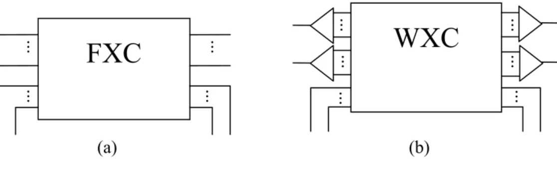
Fig. 3. Node architecture used in heterogeneous networks. (a) fxc-node. (b) wxc-node..4

Fig. 4. Architecture of three-stage MG-OXC in [7]...5

Fig. 5. Architecture two-stage MG-OXC in [8]...6

Fig. 6. Architecture of novel MG-OXC in [12]...6

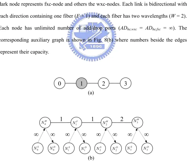
Fig. 7. Construction of auxiliary graph for homogeneous network. (a) Physical topology of the network. (b) The corresponding auxiliary graph...14

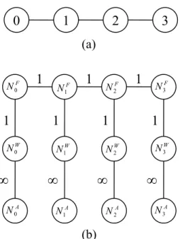
Fig. 8. Construction of auxiliary graph for heterogeneous network. (a) Physical topology of the network. (b) The corresponding auxiliary graph...16

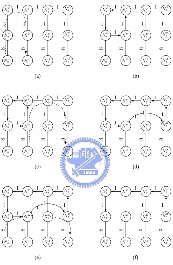
Fig. 9. (a) Path for R1. (b) Auxiliary graph updated after routing R1. (c) Path for R2. (d) Auxiliary graph updated after routing R2. (e) Path for R3. (f) Auxiliary graph updated after routing R3...18

Fig. 10. (a) Path for R1. (b) Auxiliary graph updated after routing R1. (c) Path for R2. (d) Auxiliary graph updated after routing R2...20

Fig. 11. 24-node regular topology of degree 3...26

Fig. 12. Comparison of different weight assignment policies when SRF is used...28

Fig. 13. Comparison of different weight assignment policies when LRF is used...29

Fig. 14. Comparison of different weight assignment policies when HTF is used...29

Fig. 15. Comparison of different weight assignment policies when MUF is used...30

Fig. 16. Best curves picked out from Fig. 9 ~ Fig. 12...30

Fig. 17. Comparison of different weight assignment policies when SRF is used...32

Fig. 18. Comparison of different weight assignment policies when LRF is used...32

Fig. 19. Comparison of different weight assignment policies when HTF is used...33

Fig. 20. Comparison of different weight assignment policies when MUF is used...33

Fig. 21. Best curves picked out from Fig. 14 ~ Fig. 17...34

Fig. 22. Comparison of LFPF+MUF+EV and various randomly generated combinations...35

Fig. 23. Performance comparison of the two networks under configuration 1...36

Fig. 24. Performance comparison of the two networks under configuration 2...37

(8)

List of Tables

TABLE 1. Weight Assignment Policies for Each Network...24 TABLE 2. Weight Assignments for The Three Policies Used in Homogeneous

Network...28 TABLE 3. Weight Assignments for The Three Policies Used in Heterogeneous

Network...31 TABLE 4. Network Configurations Used to Compare the Performance...36

(9)

Chapter 1. Introduction

All-optical wavelength-division-multiplexed (WDM) networks are considered to be one of the most promising future transport infrastructures to meet the ever-increasing need for bandwidth. Such networks consist of optical cross-connects (OXCs) interconnected by fiber links, with each fiber supports a number of wavelength channels. End users in the networks communicate with each other via all-optical channels, i.e., lightpaths, where each of which may span a number of fiber links to provide a “circuit-switched” interconnection between two nodes. In the absence of wavelength converters, a lightpath is required to operate on the same wavelength along all fiber links it traverses, which is known as the wavelength continuity constraint. Using wavelength converters, a lightpath may use different wavelengths on its route from its source to its destination. One of a typical problem is that given the network with limited resources and a set of lightpaths, determine the routing and wavelength assignment (RWA) of these lightpaths so that the number of the blocked requests are minimized [1]-[2].

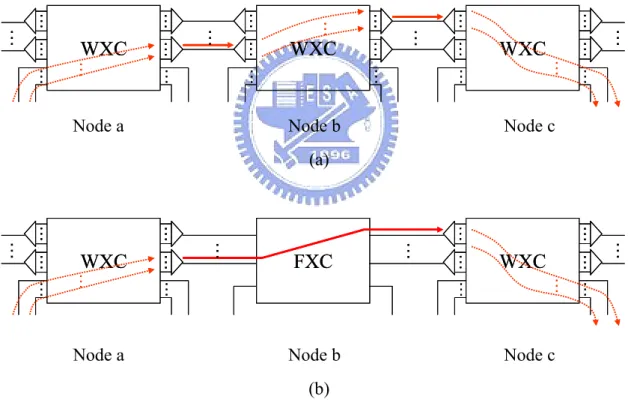
With current technologies, the huge fiber bandwidth can be divided into 100 or more wavelengths. However, as the number of wavelength channel increases, the number of ports needed at OXCs also increases, making the size of OXCs too large to implement and maintain. Recently, several types of hierarchical OXCs, or multi-granular OXCs (MG-OXCs) have been proposed to handle such scalability problem. The principle is to bundle a group of consecutive wavelength channels together and switch them as a single unit on a specific route so that the number of ports of intermediate cross-connects along the route can be reduced. Fig. 1 illustrates the

(10)

benefit of multigranularity switching. In Fig. 1(a), a set of lightpaths is to be routed from node a to node c bypassing node b. When entering node b, the fiber has to be demultiplexed into wavelengths, and the wavelengths are again multiplexed into fiber when leaving node b. To reduce the number of ports used at node b, in Fig. 1(b) the wavelength cross-connect (WXC) is replaced by fiber cross-connect (FXC) so that only one input port and one output port are used at node b. Note that the passage created by the grouped wavelengths from the point where they are multiplexed to the point where they are demultiplexed is defined as a tunnel. We can therefore view the traditional WDM networks as the networks covered with only 1-hop tunnels.

WXC

… … … …

WXC

… … … …

WXC

… … … … … … … … … … … … … …

WXC

…… …… …… ……

WXC

…… …… …… ……

WXC

…… …… …… …… … … … … … … … … … …

Node a Node b Node c

(a)

WXC

… … … …

FXC

WXC

… … … … … … … … … … … …

WXC

…… …… …… ……

FXC

WXC

…… …… …… …… … … … … … … … …

Node a Node b Node c

(b)

Fig. 1. Illustration of port saving using multigranularity switching. (a) Traditional network. (b) Network utilizing multigranularity switching.

1.1 Previous Work

(11)

MG-OXC are summarized such as small-scale modularity, reduction in cross-talk, and the reduction of complexity. In [4], similar idea is presented and is demonstrated on the WDM ring networks. Using three-stage MG-OXC architecture (Fig. 2), [5] shows that the number of ports needed, when grouping are applied to the networks, can be greatly reduced, compared to the traditional OXC solution. Single-layer architecture is proposed in [6]. In [7], employing a two-stage multiplexing scheme of waveband and wavelength (Fig. 3), an integer linear programming (ILP) formulation and a heuristic are given, but only aiming at grouping lightpaths with the same destination. In [8], both ILP and heuristic are given to handle the three-stage architecture. Grouping strategies are not constrained by any of the source-destination constraint. [9] solves the grooming problem with only two layers. To solve the problem on more than two layers, say three, the approach can be used recursively in a bottom-up manner that first groom wavelengths into bands and than bands into fibers. The authors in [10] propose two algorithms that groom the lightpaths in online and offline manners, where the difference is that the online approach considers one path at a time and the offline one all the paths at a time. In [11], the authors propose a novel MG-OXC architecture (Fig. 4) and develop two heuristics to improve the performance of the networks with dynamic traffic, with the assumption being that the network resources are fixed at the beginning. One of the heuristics dynamically set up the necessary tunnels as the request comes while the other allocates all tunnels into networks at the planning stage. Proceeding with the architecture in [11], in [12] the authors aim at dimensioning the network resources as the network traffic grows. The problem are formulated into a constraint programming (CP) process and to reduce the computation complexity, the CP is separated into two ILP processed that can be sequentially performed. The author in [13] proposed a hybrid switch architecture incorporating all-optical waveband switching and electrical TDM switching. MILP and an heuristic are presented to minimize the network switch cost.

(12)

[14] uses a Lagrangean Relaxation (LR) approach to resolve the multigranularity RWA problem considering both fiber and lambda switches.

Space-switch

Fig. 2. Architecture of three-stage MG-OXC in [7].

Fig. 3. Architecture two-stage MG-OXC in [8].

Space-switch Space-switch Drop W Drop W WXC Dro p F Dro p B D D ro p F rop B BXC FXC

Input fibers Output fibers

WXC

BXC

Input _Output Waveband Waveband Wavelength _Wavelength demux _mux fibers _fibers mux demux

(13)

Lam da Switching b Box F ib er F ib er W B S W B S B B B B L drop add w itc hin g B ox w itc hin g B ox L S w itc hin g B ox S w itc hin g B ox L L

B Waveband _{De-multiplexer} B Waveband _Multiplexer L Wavelength _{De-multiplexer} L Wavelength _Multiplexer

Fig. 4. Architecture of novel MG-OXC in [12].

1.2 Motivation and Contribution

Although various MG-OXC architectures and the corresponding heuristics have been

this paper, we make a simulation-based investigation on two types of networks with

proposed, comparison of the performance between them has not yet been extensively studied. The outcome of the comparison is helpful, for example, for the network service providers to choose the better ones for the future deployment.

In

different node architectures, with the object of choosing the better one for future deployment. More specifically, we would choose the one with better performance if both networks cost the same or about the same. Fig.5 and Fig.6 shows the node architectures used in the two networks, defined as homogeneous network and

(14)

heterogeneous network. In the homogeneous network, all the nodes are of the same

architecture, which is shown in Fig. 5. All the input/output fibers are connected to the FXC part of the node. FXC switches at the granularity of fibers and only fibers whose individual wavelengths need to be added or dropped will be demultiplexed into wavelengths, which then enter the WXC that switches at the granularity of wavelengths (F and α are described in next chapter). In the heterogeneous network, all the nodes are either of fxc-node (Fig. 6(a)) or wxc-node (Fig. 6(b)) architecture.

Fig. 5. Node architecture used in homogeneous networks.

thousands of combinations to configure a network for a fixed amount of cost. To

FXC

WXC

... ...

... ... ... ... . . . . . . . . . . . . F α⋅F (a) (b)

FXC

... ... ... ...

WXC

Fig. 6. Node architecture used in heterogeneous networks. (a) fxc-node. (b) wxc-node.

Since many parameters can be tuned to configure a network, there may exist

...

... ... ... ...

(15)

simp

1.3 Organization of the Thesis

The rest of the thesis is organized as follows. We describe our comparison methodology in Chapter 2. Chapter 3 presents the heuristics we use in our study. Chap

lify our investigation, we would make some assumptions so that the number of parameters can be greatly reduced and the cost of the network can be easily tuned. Deriving from the graph model proposed in [15], we modified the model and develop three heuristics for the two networks to reach for their best performance as possible. Simulation is conducted to support the rationality of our heuristics and to compare the performance of the two networks.

ter 4 elaborates on the pair-selection schemes and weight assignment policies used in the heuristics presented in Chapter 3. Simulation results are shown in Chapter 5. The paper concludes in Chapter 6.

(16)

Chapter 2. Methodology

This chapter describes the methodology to conduct the comparison of performance of the networks and the basic assumptions we made to simplify our study. Based on these assumptions, a cost function is derived for each of the networks.

2.1 Comparison Steps

The comparison methodology used in our study can be summarized as follows: (1) Configure the two networks to the state so that their best performance can be

achieved, while complying with the restriction that the cost of the two networks should be the same or about the same.

(2) Develop a practical heuristic for each network to route the lightpath requests. (3) Use the representing heuristics to measure the performance of each network. The metrics for the performance is the blocking probability when given in advance a set of lightpath requests to be routed.

2.2 Assumptions

As described earlier, there are too many ways to configure the network that consumes a fixed amount of cost. Thus, we make the following assumptions for the simplicity of our study:

y Each node in the network topology G(N, E), where N is the set of nodes and E the links, has the same degree d.

(17)

y Each directional link e ∈ E in the topology has the same number of fibers F. y Each fiber has the same number of wavelengths W.

y In the homogeneous network, each node has the same number of add/drop ports ADho. Each node has the same number of fiber ports, α ⋅ F ⋅ d, that connect to/from its WXC, where α ≤ 1 denotes the ratio of the number of fibers ports connecting to/from the WXC to the number of ports connecting from/to other nodes (Fig. 5).

y In the heterogeneous network, each wxc-node has the same number of add/drop ports ADhe,wxc, and each fxc-node has the same number of add/drop ports ADhe,fxc.

y Each node is assumed to have full wavelength conversion. (Therefore, the RWA problem can be reduced to a single routing problem.)

y The cost of the network is evaluated only by the number of mirrors used in the switching fabrics of all the nodes, assuming that two-dimensional (2-D) MEMS technology is used where the number of mirrors taken by a K × K switch is K2 [16].

2.3 Cost Functions of the Networks and Needed Heuristics

Base on the above assumptions, we can formulate the cost for each network as follows:

Cost of homogeneous network =

⎣

⎦

) (

⎣

⎦

) ] [( 2 2 ho AD W d F d F d F N ⋅ ⋅ + ⋅ ⋅α + ⋅ ⋅α ⋅ + (1)

Cost of heterogeneous network =

⎣

⎦

⎣

⎦

2 , 2 , ) ( ) ( ) (N − ρ⋅ N ⋅ F⋅d⋅W +AD_he_wxc + ρ⋅ N ⋅ F⋅d+AD_he _fxc (2)

(18)

where ρ in (2) is the percentage of fxc-nodes in the heterogeneous network. When configuring the network to the same or the similar cost, given |N|, d, F, W, ADho,

ADhe,wxc and ADhe,fxc, the cost of homogeneous and heterogeneous network are determined by α and ρ respectively. Note that in the heterogeneous network, even after

ρ is chosen, by which the number of fxc-nodes can be calculated, we need to further determine which nodes should be assigned as fxc-nodes among all the nodes in the network before starting to route the requests.

From the above discussion, we can summarize the heuristics we need to conduct our experiment. For each network, we need a heuristic to route the given set of lightpath requests, with the object being to minimize the blocking probability. In addition, for the heterogeneous network, before routing the requests, we need a heuristic for the fxc-node assignment when given the number of fxc-nodes to be assigned. We introduce these heuristics in Chapter 3.

(19)

Chapter 3. Heuristics for Routing the Lightpaths and

Fxc-node assignment

To satisfy the given lightpath requests, one important observation is that lightpaths are always carried in sequences of tunnels all the way from their sources to their destinations, i.e., lightpaths are routed on the virtual topology formed by tunnels. The situation is analogous to the traffic grooming problem in the traditional WDM networks, which is to determine how to set up lightpaths to satisfy the connection requests of the subwavelength granularity. Deriving from the elegant model proposed in [3], we make some modifications to the original model to make it applicable in our study. The heuristics possess the simplicity by first transform the given network resources into an auxiliary graph and then base on which shortest path algorithm is applied to route the requests, with some manipulation on the edges each time a path is found to reflect the remaining network resources. We also propose a heuristic to determine the fxc-nodes. It route the traffic on the homogeneous network and rate for each node the priority to be chosen as a fxc-node by calculating the number of fiber ports it uses.

We first introduce the method to construct the auxiliary graph for each network. Second, we describe algorithms to route a single lightpath request on their auxiliary graphs respectively and based on those algorithms, the procedure for routing a set of lightpath requests is then developed. At the end of the chapter, we elaborate on the fxc-node assignment algorithm.

(20)

3.1 Auxiliary Graphs

3.1.1 Construction of Auxiliary Graph for Homogeneous Network

Let G(N, E) and G’(N’, E’) be the graph representing the network topology and the

corresponding auxiliary graph. G’ is a graph with access, wavelength and fiber layers.

N’ is obtained by extending each Ni ∈ N , 1 ≤ i ≤ |N|, to , and , where the

super-script A, W and F means the node is on access, wavelength and fiber layer,

respectively. Each edge e

A i N W i N F i N

i ∈ E’, 1 ≤ i ≤ |E’|, has two values associated with it, cap(ei) and wt(ei), which represent the capacity and the weight of the edge respectively (we describe the weight assignment policies in Chapter 5). Edges in E’ can be categorized

and added to G’ as follows:

y Fiber edge (FE)

There is an edge from to , 1 ≤ i, j ≤ |N|, if there are unused fibers from node i to node j. The capacity of the edge corresponds to the number of

these unused fibers.

F i

N F

j

N

y Fiber port mux edge (FPME)

There is an edge from to , 1 ≤ i ≤ |N|, if there are unused multiplexers at node i. The capacity of the edge corresponds to the number of

these unused multiplexers.

W i

N F

i N

y Fiber port demux edge (FPDE)

There is an edge from to , 1 ≤ i ≤ |N|, if there are unused demultiplexers at node i. The capacity of the edge corresponds to the number

F i

N W

i N

(21)

of these unused demultiplexers.

y Wavelength add edge (WAE)

There is an edge from to , 1 ≤ i ≤ |N|, if there are unused add ports at node i connecting from its access station. The capacity of the edge

corresponds to the number of these unused add ports.

A i

N W

i N

y Wavelength drop edge (WDE)

There is an edge from to , 1 ≤ i ≤ |N|, if there are unused drop ports at node i connecting to its access station. The capacity of the edge corresponds

to the number of these unused drop ports.

W i

N A

i N

y Tunnel edge (TE)

There is an edge from to , 1 ≤ i, j ≤ |N|, if there are unused wavelengths in the established tunnels with ingress at node i and egress at

node j. The capacity of the edge corresponds to the number of the unused

wavelengths in these tunnels.

W i

N W

j

N

Fig. 7 illustrates how to initialize the auxiliary graph for the homogeneous network given the network configuration. Fig. 7(a) is the physical topology of the network. Each link is bidirectional with each direction containing one fiber (F = 1) and each fiber has

two wavelengths (W = 2). Each node’s FXC has only one port connecting to/from its

WXC (α = 50%), and each WXC has unlimited number of add/drop ports (ADho = ∞). The auxiliary graph is shown in Fig. 7(b) where numbers beside the edges represent their capacity.

(22)

Fig. 7. Construction of auxiliary graph for homogeneous network. (a) Physical topology of the network. (b) The corresponding auxiliary graph.

3.1.2 Construction of Auxiliary Graph for Heterogeneous Network

Let G(N, E) and G’’(N’’, E’’) be the graph representing the network topology and

the corresponding auxiliary graph. G’’ is a graph with access layer and OXC layer. N’’ is

obtained by extending each Ni ∈ N , 1 ≤ i ≤ |N|, to and , plus or depending on the type of node i, where the super-script S and D means the node is on

source and destination side of access layer, and W and F means the type of the node is

fxc-node and wxc-node. Each edge e

S i N D i N W i N F i N

i ∈ E’’, 1 ≤ i ≤ |E’’|, has two values associated with it, cap(ei) and wt(ei), which means the capacity and the weight (described in Chapter 5) of the edge respectively. Edges in E’’ can be categorized and added to G’’ as follows:

y Fiber edge from wxc-node to fxc-node (FEwf)

There is an edge from W to , 1 ≤ i, j ≤ |N|, if there are unused fibers

i N F j N 0 1 2 3 (a) (b) F N0 F N3 F N2 A N2 A N0 N1A A N3 W N3 W N2 W N1 W N0 1 _NF 1 1 1 1 1 1 1

∞

(23)

from node i to node j. The capacity of the edge corresponds to the number of

y Fiber edge from fxc-node to wxc-node (FEfw)

F i

N W

j

N

y Fiber edge from fxc-node to fxc-node (FEff)

F i

N F

j

N

y Wavelength add edge (WAE)

There is an edge from to , 1 ≤ i, j ≤ |N|, if there are unused add ports at node i connecting from the its access station. The capacity of the edge

corresponds to the number of these unused ports.

S i

N W

i N

y Wavelength drop edge (WDE)

There is an edge from to , 1 ≤ i ≤ |N|, if there are unused drop ports at node i connecting to its access station. The capacity of the edge corresponds

to the number of these unused ports.

W i

N D

i N

y Fiber add edge (FAE)

There is an edge from to , 1 ≤ i, j ≤ |N|, if there are unused ports at node i connecting from its access station. The capacity of the edge

corresponds to the number of these unused ports.

S i

N F

i N

y Fiber drop edge (FDE)

There is an edge from F to , 1 ≤ i ≤ |N|, if there are unused drop ports

i

N D

i N

(24)

at node i connecting to its access station. The capacity of the edge corresponds

to the number of these unused ports.

y Tunnel edge (TE)

There is an edge from to ,1 ≤ i, j ≤ |N|, to , 1 ≤ i, j ≤ |N|, or to ,1 ≤ i, j ≤ |N|, if there are unused wavelengths in the tunnels with ingress at node i and egress at node j. The capacity of the edge

corresponds to the number of these unused wavelengths in these tunnels.

W i N W j N S i N W j N W i N D j N

Fig. 8 is the example. Fig. 8(a) is the physical topology of the network in which the dark node represents fxc-node and others the wxc-nodes. Each link is bidirectional with each direction containing one fiber (F = 1) and each fiber has two wavelengths (W = 2).

Each node has unlimited number of add/drop ports (ADhe,wxc = ADhe,fxc = ∞). The corresponding auxiliary graph is shown in Fig. 8(b) where numbers beside the edges represent their capacity.

0

1

2

3

(a)

k. (a) Phys Fig. 8. Construction of auxiliary graph for heterogeneous networ ical topology of the network. (b) The corresponding auxiliary graph.

S N0 N2S S N3

1

1 ∞

∞

W N0 D N0 N1S D N1 F N1 W N2 D N2 W N3

2

D N3

∞

(b)

(25)

3.2 Algorithms to Route the Requests

3.2.1 Auxiliary Graph Based Grooming Algorithm for Homogeneous Network

To route a request, denoted by R(i, j), where i and j are the source and destination

Continue with the example in Fig. 7, Fig. 9 shows the process of routing three cons

(AGGA-HO)

nodes, it has to find a path for the request on the auxiliary graph and if successful, the edges and their associative capacities have to be updated. Following is the detail of the algorithm. Algorithm AGGA-HO R(i, j). to on G’. If failed, d i i i

Input: A lightpath request

Step1. Find the shortest path p from A i

N A

j

N

return 0.

Step2. Let [e1, e2, …, eh] be the sequence of edges traversed by p, an set i = 1.

Step3. Decrease cap(e ) by 1. If cap(e ) = 0, remove e from G’.

∈

Step4. If ei WFPE, let x be the start point of ei. Go to Step 6. ∈

Step5. If ei FWPE, let y be the ending point of ei and add an edge

y G’ W

from x to on with capacity – 1.

Step6. Increase i by 1. If i > h, return 1, otherwise go to Step 3.

ecutive requests, R1(0, 1), R2(1, 3) and R3(0, 3). Note that R3 utilizes the tunnels

(26)

1

Fig. 9. (a) Path for R1. (b) Auxiliary graph updated after routing R1. (c) Path for R2. (d)

Auxiliary graph updated after routing R2. (e) Path for R3. (f) Auxiliary graph updated

after routing R3. (f) 1 F N0 F N3 F N2 A N2 A N0 N1A A N3 W N3 W N2 W N1 W N0 1 1 1 1 1 ∞ ∞ ∞ ∞ F N1 (e) 1 F N0 F N3 F N2 A N2 A N0 N1A A N3 W N3 W N2 W N1 W N0 1 ₁ 1 1 1 ₁ ∞ ∞ ∞ ∞ 1 F N1 (d) 1 F N0 F N3 F N2 A N2 A N0 N1A A N3 W N3 W N2 W N1 W N0 1 ₁ 1 1 1 ₁ ∞ ∞ ∞ ∞ 1 F N1 (c) 1 F N0 F N3 F N2 A N2 A N0 N1A A N3 W N3 W N2 W N1 W N0 1 1 1 1 1 1 ∞ ∞ ∞ ∞ 1 F N1 (b) F N0 F N3 F N2 A N2 A N0 N1A A N3 W N3 W N2 W N1 W N0 1 1 1 1 1 1 ∞ ∞ ∞ ∞ 1 F N1 (a) A N0 F N0 F N3 F N2 F N1 A N2 A N1 A N3 W N3 W N2 W N1 W N0 1 1 1 1 1 1 1 ∞ ∞ ∞ ∞

(27)

3.2.2 Auxiliary Graph Based Grooming Algorithm for Heterogeneous Network (AGGA-HE)

Similar to AGGA-HO, below is the algorithm to route a single request on the heterogeneous network.

Algorithm AGGA-HE

Input: A lightpath request R(i, j).

Step1. Find the shortest path p from to on G’’. If failed,

return 0. S i N D j N

Step2. Let [e1, e2, …, eh] denote the sequence of edges traversed by p, and set i = 1.

Step3. Decrease cap(ei) by 1 and if cap(ei) = 0, remove ei from G’. Step4. If ei ∈ FAE or ei ∈ FEwf, let x be the start point of ei. Go to step

6.

Step5. If ei ∈ FDE or ei ∈ FEff, let y be the end point of ei and add an edge from x to y on G’ with capacity W-1.

Step6. Increase i by 1. If i > h, return 1, otherwise go to Step 3.

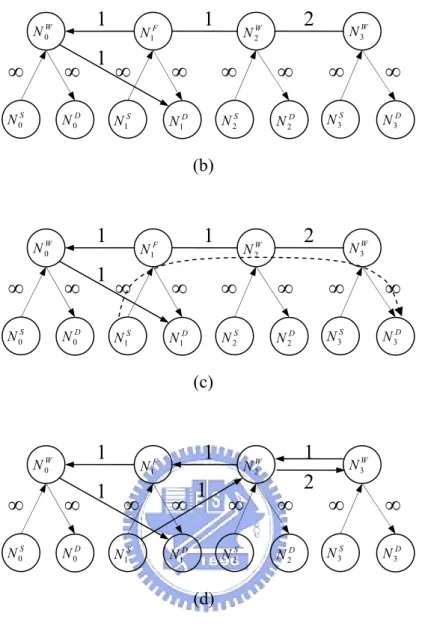
Similarly, continue with Fig. 8, Fig. 10 is the example on routing R1(0, 1), R2(1, 3)

and R3(0, 3). Note that R3 is blocked since there exists no path on the auxiliary graph

from _NS to after R

0 N3D 1 and R3 are routed.

S N0 N2S S N3

1

1 ∞

∞

W N0 D N0 S N1 N1D F N1 W N2 D N2 W N3

2

D N3

∞

(a)

(28)

S

N0 N2S

S

N3

1

Fig. 10. (a) Path for R1. (b) Auxiliary graph updated after routing R1. (c) Path for R2. (d)

Auxiliary graph updated after routing R2.

3.2.3 Modified Integrated Grooming Procedure (MINGPROC)

The procedure, Modified Integrated Grooming Procedure (MINGPROC), modified from [3], is used to route the set of requests for both networks. It simply sorts the requests in a specific order and then route the requests sequentially in that order by repeating the algorithm that route only one single request.

S N0 N2S S N3

1

1 ∞

∞

W N0 D N0 N1S D N1 F N1 W N2 D N2 W N3 D N3

1 ∞

∞

1

2

(d) S N0 N2S S N3

1

1 ∞

∞

W N0 D N0 N1S N1D F N1 W N2 D N2 W N3 D N3

2 ∞

∞

1

(c)

∞

W N0 D N0 S N1 N1D F N1 W N2 D N2

2

_NW 3 D N3

∞

1 ∞

∞

(b)

(29)

Procedure MINGPROC

Input: network configuration and a set of lightpath requests Step1. Construct the corresponding auxiliary graph.

Step2. Sort the source-destination pair order according to one of the pair-selection schemes.

Step3. Apply AGGA-HO/AGGA-HE to route the lightpath requests in the sequence determined by Step 2.

We describe the pair-selection schemes in Chapter 5.

3.3 Fxc-node Assignment

Given ρ, thus the number of nodes to be assigned as fxc-nodes, we need to determine the allocation of these nodes so that better routing effect can be achieved. We propose a simple algorithm, Least Fiber Port First (LFPF), to solve the problem. Since fxc-nodes switch at the granularity of the whole fiber, they should be carefully allocated to minimize the impairment brought by the reduction in their switching flexibility. It is reasonable to assign the node a fxc-node if few input fiber and output fiber ports are used at that node, which may result from 1) lightpaths densely bundled in a input fiber remain bundled as they are and are switched to the same output fiber port 2) only a few lightpaths bypass, start from, and end at that node. LFPF captures the idea by assuming that the network is of homogeneous network architecture and route the traffic on it. The node that uses least fiber ports gets the highest priority to be chosen as the fxc-node. The whole LFPF works as follows.

(30)

Algorithm LFPF

Input: k (number of fxc-nodes to be assigned).

Step1. Randomly generate a traffic matrix with sufficiently large load. Step2. Apply MINGPROC to route the traffic on the homogeneous

network with α = 100%.

Step3. For each node, calculate the sum of used fiber input ports and fiber output ports, denoted by fp.

Step4. Repeat Step 1~Step 3 100 times

Step5. Average fp for each node and the first k nodes with least fp are

(31)

Chapter 4. Pair-Selection Scheme and Weight Assignment

Policies

4.1 Pair-Selection Schemes

Pair-selection schemes are used to determine the order the requests are routed. More specifically, all the source-destination pairs are first sorted in an specific order and starting from the first pair until the last pair, all the requests for that pair will be routed. If blocking occurs in the process, it directly moves to the next pair. We provide four pair-selection schemes used to determine the pair order.

y Shortest Route First (SRF). SRF sort the pairs in the non-decreasing order

according to their physical hops.

y Longest Route First (LRF). LRF sort the pairs in the non-increasing order

according to their physical hops.

y Heaviest Traffic First (HTF). HTF sort the pairs in the non-decreasing order

according to their number of requests.

y Maximum Utilization First (MUF). MUF sort the pairs in the

non-decreasing order according to their utilization, which is defined as the number of requests for the pair divided by the number of physical hops of the pair.

4.2 Weight Assignment Policies

Applying different weight functions to the graph model would result in different routing effect. We provide three weight assignment policies for each network. Table 1

(32)

lists the policies used for each network.

TABLE 1

WEIGHT ASSIGNMENT POLICIES FOR EACH NETWORK Homogeneous Network Heterogeneous Network Minimum Tunnel (MT) Minimum Tunnel (MT) Minimum Fiber (MF) Minimum Fiber (MF) Less Logical Hop (LLH) Equal Value (EV)

y Minimum Tunnel (MT). MT is the policy that tries to construct minimum

number of tunnels whenever routing a request. For homogeneous network, this can be achieved by assigning the weight of FPME and FPDE to a very large value, and for heterogeneous network, the weight of FAE, FDE, FEwf

and FEfw to a very large value.

y Minimum Fiber (MF). MT is the policy that consumes minimum number of

unused fibers whenever routing a request. For homogeneous network, this can be achieved by assigning the weight of FE to a very large value. For heterogeneous network, the weight of FEff, FEwf and FEfw is set to a very large

value. Note that the fibers that connect two wxc-nodes are excluded since they are viewed as the 1-hop tunnels.

y Less Logic Hops (LLH). LLH is designed for homogeneous networks. LLH

assigns the weight of FPME and FPDE to 0, and if TE is to m, m > 0, then FE

is set to k⋅m − ε, where k ∈ Z, k > 1 and ε is a very small value. The potential meaning is that LLH would prefer to walk through a fiber edge that weighs

(33)

k⋅m − ε rather than to walk through k hops of tunnel edges that weigh totally

k⋅m.

y Equal Value (EV). EV is designed for heterogeneous networks. EV assigns

FEwf, FEfw, FEff and TE to the same weight, and assigns the weight of FAE

and FDE to a much smaller value. The potential meaning is just to let FEwf,

(34)

Chapter 5. Simulation Results

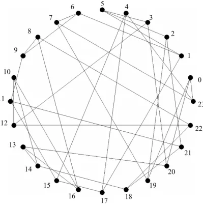
The simulation is conducted on the 24-node network shown in Fig. 11, which is a regular graph of degree 3 generated randomly. The request set is randomly generated in a way that the number of requests for each pair is r ⋅ λ, where r is a random number in

the range [0.5, 1,5] and λ is the constant representing the average number of requests for every pair. Note that r ⋅ λ is rounded off to the nearest integer.

5 6 4 7 3 8 ₂ 9 1 10 0 11 23 12 22 13 21 14 ₂₀ 15 19 16 ₁₇ 18

(35)

5.1 Finding Representing Heuristic for Homogeneous Networks

We try different combination of pair-selection schemes and weight assignment policies, and the combination that result in the best performance among them is chosen to be used in the later comparison of the two networks. We assume F = 4, W = 16, α = 80% and ADho = ∞. Weight assignment for each policy is listed in Table 2. Note that for the LLH, m is set to 10 and k to 2 (mentioned in Chapter 5). We examine the blocking

probability for various λ. Fig. 12 ~ Fig. 15 show the results when using different weight assignment policies under fixed pair-selection schemes. It can be observed that LLH always performs best for each of the pair-selection schemes. The drawback of MT is that it allocates minimum number of tunnels as possible, which result in less lightpaths can be accommodated. The drawback of MF is that it treasures fibers too much such that each lightpath request would try to utilize the existing tunnels as possible, which means that more tunnels are used to accommodate the lightpath. Fig. 16 picks the best curves from Fig. 12 ~ Fig. 15 to show that SRF + LLH is the best among them. The results indicate that short tunnels will be allocated first to increase basic routing flexibility, and then with LLH to help to increase the additional network connectivity. Longer tunnels should not be allocated fist since fiber capacity may be used up too fast such that later tunnels can not be allocated. Note that there is not much difference between SRF + LLH and MUF + LLH. This is because the requests generated are uniformly distributed between each node pair, thus, by the definition of MUF, it would still prefer the pair with short physical hop length.

(36)

TABLE 2

WEIGHT ASSIGNMENTS FOR THE THREE IES USED IN HOMOGENEOUS NETW

POLIC ORK MT MF LLH FE 5 1000 19 FPME 1000 0 0 FPDE 1000 0 0 WAE 1 1 1 WDE 1 1 1 TE 1 1 10 0 0.05 0.1 0.15 0.2 0.25 0.3 0.35 1.4 1.6 1.8 2 2.2 λ blo ckin g pro babi lity SRF+MT SRF+MF SRF+LLH

(37)

0 0.05 0.1 0.15 0.2 0.25 0.3 0.35 0.4 0.45 1.4 1.6 1.8 2 2.2 λ blo ckin g pro babi lity LRF+MT LRF+MF LRF+LLH

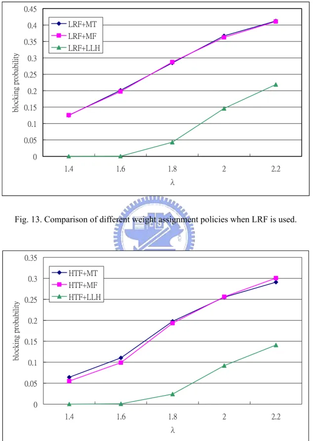
Fig. 13. Comparison of different weight assignment policies when LRF is used.

0 0.05 0.1 0.15 0.2 0.25 0.3 0.35 1.4 1.6 1.8 2 2.2 λ block ing p robab ility HTF+MT HTF+MF HTF+LLH

(38)

0 0.05 0.1 0.15 0.2 0.25 0.3 1.4 1.6 1.8 2 2.2 λ block ing p robab ility MUF+MT MUF+MF MUF+LLH

Fig. 15. Comparison of different weight assignment policies when MUF is used.

0 0.05 0.1 0.15 0.2 0.25 1.4 1.6 1.8 2 2.2 λ block ing p robab ility SRF+LLH LRF+LLH HTF+LLH MUF+LLH

(39)

5.2 Finding Representing Heuristic for Heterogeneous Networks

We try different combination of fxc-node allocation, pair-selection schemes and weight assignment policies. We first obtain the best combination of pair-selection scheme and weigh assignment when LFPF is used to determine fxc-nodes. We assume F

= 4, W = 16, ρ = 50%, ADhe,wxc = ADhe,fxc = ∞. Weight assignment for each policy is listed in Table 3. Fig. 17 ~ Fig. 20 is the result with assumption that LFPF is used to determine the fxc-nodes and it shows that EV always performs best under each of the pair-selection schemes. This may result from that by treating all the fibers equally, fibers can be used more fairly than MT and MF. Fig. 21 picks the best curves from Fig. 17 ~ Fig. 20 to show that MUF + EV is the best among them. Again, MUF + EV and SRF + EV have similar performance because MUF and SRF both choose the pair with shortest physical hop length to be routed first.

TABLE 3

WEIGHT ASSIGNMENTS FOR THE THREE IES USED IN HETEROGENEOUS NETW

POLIC ORK MT MF EV FEwf 1000 1000 10 FEfw 1000 1000 10 FEff 10 1000 10 WAE 1 1 1 WDE 1 1 1 FAE 1000 1 1 FDE 1000 1 1 TE 10 10 10

(40)

0 0.05 0.1 0.15 0.2 0.25 0.3 0.35 0.4 1.4 1.6 1.8 2 2.2 λ blocking probability SRF+MT SRF+MF SRF+EV

Fig. 17. Comparison of different weight assignment policies when SRF is used.

0 0.05 0.1 0.15 0.2 0.25 0.3 0.35 0.4 0.45 0.5 1.4 1.6 1.8 2 2.2 λ blo ckin g pro babi lity LRF+MT LRF+MF LRF+EV

(41)

0 0.05 0.1 0.15 0.2 0.25 0.3 0.35 0.4 1.4 1.6 1.8 2 2.2 λ blocking probability HTF+MT HTF+MF HTF+EV

Fig. 19. Comparison of different weight assignment policies when HTF is used.

0 0.05 0.1 0.15 0.2 0.25 0.3 0.35 1.4 1.6 1.8 2 2.2 λ blo ckin g pro babi lity MUF+MT MUF+MF MUF+EV

(42)

0 0.05 0.1 0.15 0.2 0.25 1.4 1.6 1.8 2 2.2 λ blocking probability SRF+EV LRF+EV HTF+EV MUF+EV

Fig. 21. Best curves picked out from Fig. 14 ~ Fig. 17.

Now, we would verify that LFPF performs acceptably good comparing to other fxc-node placement. Let MUF and EV be the pair-selection schem and weight assignment policy. randi denote the i-th experiment in which fxc-nodes are randomly

assigned. Fig. 22 shows the result of rand1~rand4 and LFPF. It shows that LFPF has lower blocking probability compared to rand1~rand4.

(43)

0 0.05 0.1 0.15 0.2 0.25 1 2 3 4 5 λ blocking pr ob ability rand1 rand2 rand3 rand4 LFPF

Fig. 22. Comparison of LFPF and other random fxc-nodes placements.

5.3 Comparison of the two networks

We assume F = 4 and W = 16. Let λmax denotes the maximum λ conducted in the experiment. ADho and ADhe,wxc are set to (1.5 ⋅ λmax) ⋅ (|N| - 1) so that requests are not blocked even before routing. ADhe,wxc is set to F ⋅ d. Then, α and ρ are tuned to make the cost of the two network near the same. Table 4 shows the network configurations we use to compare the performance of the two networks. Simulation results are show in Fig. 23 ~ Fig. 25. It is obvious that the heterogeneous networks outperforms the homogeneous network for each of the three configurations. For λ = 2, for example, the blocking probability of heterogeneous network is 24%, 30% and 30% less for configuration 1 ~ 3 respectively.

(44)

TABLE 4

NETWORK CONFIGURATIONS USED TO COMPARE THE PERFORMANCE Networks α /ρ # of MEMS Homogeneous 84% 1270200 Configuration 1 Heterogeneous 21% 1297179 Homogeneous 75% 1099440 Configuration 2 Heterogeneous 34% 1094544 Homogeneous 67% 941016 Configuration 3 Heterogeneous 42% 959454 Configuration 1 0 0.02 0.04 0.06 0.08 0.1 0.12 1.8 1.9 2 2.1 2.2 λ blocking probab ility homo-

(45)

Configuration 2 0 0.02 0.04 0.06 0.08 0.1 0.12 1.8 1.9 2 2.1 2.2 λ blocking probab ility homo-

hetero-Fig. 24. Performance comparison of the two networks under configuration 2.

Configuration 3 0 0.02 0.04 0.06 0.08 0.1 0.12 0.14 1.8 1.9 2 2.1 2.2 λ bl o ck in g p ro b ab ility homo-

(46)

The result is unexpected since as MG-OXCs are becoming a trend to resolve the large traffic growth, it may be more cost-effective to replace only some of the nodes in the network with OXCs that switch at different granularity rather than to replace them all with the new architecture. When designing the networks, network designers should take into account the homogeneity and heterogeneity of the networks to make the best profit.

(47)

Chapter 6. Conclusion and Future Work

We investigated the problem of choosing the more cost-effective one among two types of hierarchical cross-connect WDM networks for future deployment. We modified the graph model presented in [3] to make it applicable to our network architectures. The model transform the given network resources into an auxiliary graph and then base on which shortest path algorithm is applied to route the requests, with some manipulation on the edges each time a path is found to reflect the remaining network resources. We also proposed an effective heuristic to determine which nodes should be assigned fxc-nodes given the number of fxc-nodes to be assigned. Simulation is conducted to determine what pair-selection schemes, weight assignment policies and fxc-node assignment should be used for the networks to reach their better performance. For the homogeneous network, it shows that SRF + LLH performs best, and for the heterogeneous network, LFPF + MUF + EV. The results of the performance comparison of the two networks show that heterogeneous network outperforms homogeneous network by about 30% for the average traffic loading and thus is more preferable for the future deployment. Network designers are recommended to take into account the homogeneity and heterogeneity of the networks when designing the networks.

Finally, we remark that there remains some space to be improved for our work. For example, to get better performance, one can determine the order of the requests to be routed dynamically according to the network state but not fixed at the beginning, at the expense of higher time complexity. The weights of the edges, on the other hand, can also be assigned dynamically that take load balancing into account. In this study we assume that the networks have full wavelength conversion. In the near future, the model

(48)

may be extended to consider limited wavelength conversion and even to determine the placement of wavelength converters.

(49)

References

[1] I. Chlamtac, A. Ganz, and G.. Karmi, “Lightpath communications: an approach to high bandwidth optical WAN's,” IEEE Transactions on Communications, vol. 40,

no. 7, July, 1992, pp. 1171-1182.

[2] B. Mukherjee, “WDM optical communication networks: progress and challenges,”

IEEE Journal on Selected Areas in Communications, vol. 18, no. 10, Oct. 2000, pp.

1810-1824.

[3] K. Harada, K. Shimizu, T. Kudou, and T. Ozeki, “Hierarchical optical path cross-connect systems for large scale WDM networks,” Proc. OFC’99, vol. 2, Feb.

1999, pp. 356-358.

[4] O. Gerstel, R. Ramaswami, and W. K. Wang, “Making use of a two stage multiplexing scheme in a WDM network,” Proc. OFC’00, vol. 3, March 2000, pp.

44-46.

[5] L. Noirie, M. Vigoureux, and E. Dotaro, “Impact of intermediate traffic grouping on the dimensioning of multi-granularity optical networks,” Proc. OFC’01, vol. 2,

Mar. 2001, pp. TuG3.1-TuG3.3.

[6] R. Lingampalli and P. Vengalam, “Effect of wavelength and waveband grooming on all-optical networks with single layer photonic switching,” Proc. OFC’02,

March 2002, pp. 501-502.

[7] M. Lee, J. Yu, Y. Kim, C. Kang, and J. Park, “Design of hierarchical crossconnect WDM networks employing a two-stage multiplexing scheme of waveband and wavelength,” IEEE Journal on Selected Areas in Communications, vol. 20, no. 1,

Jan. 2002, pp. 166-171.

[8] X. Cao, V. Anand, Y. Xiong, and C. Qiao, “Performance evaluation of wavelength band switching in multifiber all-optical networks,” Proc. IEEE INFOCOM’03, vol.

(50)

3, Apr. 2003, pp. 2251-2261

[9] G. Huiban, S. Perennes, and M. Syska, “Traffic grooming in WDM networks with multi-layer switches,” Proc. IEEE International Conference on Communications (ICC’02), vol. 5, Apr. 2002, pp. 2896-2901.

[10] Y. Suemura, I. Nishioka, Y. Maeno, S. Araki, R. Izmailov, and S. Ganguly, “Hierarchical routing in layered ring and mesh optical networks,” Proc. IEEE International Conference on Communications (ICC’02), vol. 5, Apr. 2002, pp.

2727-2733.

[11] P. Ho and H. Mouftah, “Routing and wavelength assignment with multigranularity traffic in optical networks,” Journal of Lightwave Technology, vol. 20, no. 8, Aug.

2002, pp. 1292-1303.

[12] P. Ho, H. Mouftah, and J. Wu, “A scalable design of multigranularity optical cross-connects for the next-generation optical Internet,” IEEE Journal on Selected Areas in Communications, vol. 21, no. 7, Sept. 2003, pp. 1133-1142.

[13] S. Yao, C. Ou, and B. Mukherjee, “Design of hybrid optical networks with waveband and electrical TDM switching,” Proc. IEEE GLOBECOM’03, vol. 5,

Dec. 2003, pp. 2803-2808.

[14] S. Lee, M. Yuang, P. Tien, and S. Lin, “Optical tunnel allocation for WDM networks with multi-granularity switching capabilities,” IEEE GLOBECOM’03,

vol. 5, Dec. 2003, pp. 2730-2734.

[15] H. Zhu, H. Zang, K. Zhu, and B. Mukherjee, “A novel generic graph model for traffic grooming in heterogeneous WDM mesh networks,” IEEE/ACM Transactions on Networking, vol. 11, no. 2, Apr. 2003, pp. 285-299.

[16] G. Shen, T. H. Cheng, S. K. Bose, C. Lu, and T. Y. Chai, “Architectural design for multistage 2-D MEMS optical switches,” IEEE Journal of Lightwave Technology,

多單位交換在階層式光交換器光纖網路下之效能分析

國

立

交

通

大

學

資訊科學系

碩 士 論 文

多 單 位 交 換 在 階 層 式 光 交 換 器 光 纖 網 路 下 之 效 能 分 析

Performance Evaluation of Multigranularity Switching in

Hierarchical Cross-Connect WDM Networks

研 究 生：陳盈羽

指導教授：陳健 教授

多單位交換在階層式光交換器光纖網路下之效能分析

Performance Evaluation of Multigranularity Switching in Hierarchical

Cross-Connect WDM Networks

研 究 生：陳盈羽 Student：Ying-Yu Chen

指導教授：陳 健

Advisor：Chien Chen

國 立 交 通 大 學

資 訊 科 學 系

碩 士 論 文

多單位交換在階層式光交換器光纖網路下之效能分析

中文摘要

Performance Evaluation of Multigranularity Switching

in Hierarchical Cross-Connect WDM Networks

Abstract

誌謝

Table of Contents

List of Figures

List of Tables

Chapter 1. Introduction

WXC

WXC

WXC

WXC

WXC

WXC

WXC

FXC

WXC

WXC

FXC

WXC

1.1 Previous Work

WXC

BXC

1.2 Motivation and Contribution

FXC

WXC

... ...

FXC

WXC

1.3 Organization of the Thesis

Chapter 2. Methodology

2.1 Comparison Steps

2.2 Assumptions

2.3 Cost Functions of the Networks and Needed Heuristics

⎣

⎦

⎣

⎦

⎣

⎦

⎣

⎦

Chapter 3. Heuristics for Routing the Lightpaths and

Fxc-node assignment

3.1 Auxiliary Graphs

∞

∞

∞

∞

0

1

2

3

1

1

碩士論文

多單位交換在階層式光交換器光纖網路下之效能分析

研究生：陳盈羽

指導教授：陳健教授

研究生：陳盈羽 Student：Ying-Yu Chen

指導教授：陳健

國立交通大學

資訊科學系

碩士論文