Sedimentation Velocity and Potential in Concentrated Suspensions
of Charged Spheres with Arbitrary Double-Layer Thickness
Huan J. Keh1and Jau M. Ding
Department of Chemical Engineering, National Taiwan University, Taipei 106-17, Taiwan, Republic of China
E-mail: [email protected] Received January 31, 2000; accepted April 17, 2000
The sedimentation in a homogeneous suspension of charged spherical particles with an arbitrary thickness of the electric double layers is analytically studied. The effects of particle interactions are taken into account by employing a unit cell model. Overlap of the double layers of adjacent particles is allowed, and the polarization effect in the double layer surrounding each particle is considered. The electrokinetic equations that govern the ionic concentration distributions, the electric potential profile, and the fluid flow field in the electrolyte solution in a unit cell are linearized assuming that the system is only slightly distorted from equilibrium. Using a perturbation method, these linearized equations are solved for a symmetrically charged electrolyte with the surface charge density (or zeta potential) of the particle as the small perturbation parame-ter. An analytical expression for the settling velocity of the charged sphere in closed form is obtained from a balance among its gravita-tional, electrostatic, and hydrodynamic forces. A closed-form for-mula for the sedimentation potential in a suspension of identical charged spheres is also derived by using the requirement of zero net electric current. Our results demonstrate that the effects of over-lapping double layers are quite significant, even for the case of thin double layers. °C2000 Academic Press
Key Words: spherical particle; sedimentation velocity;
sedimen-tation potential; concentrated suspension; unit cell model.
1. INTRODUCTION
The sedimentation of charged colloidal particles in electrolyte solutions has received quite an amount of attention in the past. This problem is more complex than that of uncharged particles because the electric double layer surrounding each particle is distorted by the fluid flow around the particle. The deformation of the double layer resulting from the fluid motion is usually referred to as the relaxation effect (or the effect of double-layer polarization) and gives rise to an induced electric field. The sedimentation potential, which arises in a suspension of settling charged particles, was first reported by Dorn in 1878, and this effect is often known by his name (1, 2). The sedimentation
1To whom correspondence should be addressed.
potential gradient (which is of the order 1–10 V/m) not only alters the velocity and pressure distributions in the fluid due to its action on the electrolyte ions but also retards the settling of the particles by an electrophoretic effect.
An important contribution to the sedimentation theory for a dilute suspension of identical spherical particles with arbitrary double-layer thickness was made by Booth (1). Without consid-ering the particle–particle interaction effects, he solved a set of electrokinetic differential equations using a regular perturbation method to obtain formulas for the sedimentation velocity and sedimentation potential expressed as power series in the zeta potential (ζ) of the dielectric particles up to O(ζ2) and O(ζ), respectively. Numerical results relieving the restriction of low surface potential in Booth’s analysis were reported by Stigter (3) using a modification of the theory of electrophoresis of a nonconducting sphere developed by Wiersema et al. (4). It was found that the Onsager reciprocal relation between the sedimen-tation potential and the electrophoretic mobility derived by de Groot et al. (5) is satisfied within good computational accuracy. Taking the double-layer distortion from equilibrium as a small perturbation, Ohshima et al. (6) obtained general expressions and presented numerical results for the sedimentation velocity and potential in a dilute suspension of identical charged spheres over a broad range of zeta potential and double-layer thick-ness. Recently, Booth’s perturbation analysis was extended to the derivation of the sedimentation velocity and potential of charged porous spheres (7) and charged composite spheres (8) with a low density of the fixed charges. Other than cases of spherical parti-cles, the effect of the deformation of the ion cloud surrounding a charged circular cylinder on the sedimentation velocity of the particle has also been investigated semianalytically (9, 10).
In practical applications of sedimentation, relatively concen-trated suspensions of particles are usually encountered, and ef-fects of particle interactions will be important. To avoid the difficulty of the complex geometry appearing in assemblages of particles, unit cell models, which apply strictly only to periodic arrays, were often employed to predict the effects of particle in-teractions on the mean sedimentation rate in a bounded suspen-sion of identical uncharged spheres (11). These models involve
540 0021-9797/00 $35.00
Copyright°C2000 by Academic Press All rights of reproduction in any form reserved.
the concept that an assemblage can be divided into a number of identical cells, one sphere occupying each cell at its center. The boundary value problem for multiple spheres is thus reduced to the consideration of the behavior of a single sphere and its bounding envelope. The most acceptable of these models with various boundary conditions at the outer (virtual) surface of the cell are the so-called “free-surface” model due to Happel (12) and “zero-vorticity” model due to Kuwabara (13), the predic-tions of which have been tested against the experimental data. Using the Kuwabara cell model with the condition of zero net electric current, Levine et al. (14) derived analytical expressions for the sedimentation velocity and potential in a suspension of identical charged spheres with small surface potential as func-tions of the fractional volume concentration of the particles. In the limiting case of a dilute suspension, their result somewhat differs from that obtained by Booth (1), which is not subject to the constraint of zero net current. Recently, the Kuwabara cell model was also used by Ohshima (15) to demonstrate the Onsager relation between the sedimentation potential and the electrophoretic mobility of charged spheres with low zeta po-tentials in concentrated suspensions.
The analyses of Levine et al. and Ohshima were based on the assumption that the overlap of the electric double layers of adjacent particles is negligible on the virtual surface of the unit cell. With this assumption, the effect of the relaxation of the diffuse ions in the double layer within a cell due to the sedimen-tation of the particle can only be described by simple approxi-mations. Therefore, the application of their results is restricted to the case of charged spheres with relatively thin double lay-ers (say,κa ≥ 10, where κ−1is the Debye screening length and
a is the particle radius). On the other hand, the Kuwabara cell
model was chosen in these studies because it predicts that the electrophoretic mobility in a bounded suspension of identical spheres withκa → ∞ is independent of the volume fraction of particles, while the prediction of the Happel cell model gives a weak dependency of the mobility on the particle concentration (16), and because it is consistent with the irrotational-flow envi-ronment generated by an electrophoretic particle withκa → ∞ (17). In the analysis based on the concepts of interactions be-tween pairs of electrophoretic spheres and statistical mechanics (18, 19) and in a careful experimental investigation (20), how-ever, it was found that the electrophoretic mobility of a bounded suspension of identical spheres at largeκa decreases gradually rather than remains unchanged with increasing volume fraction of particles. Also, the fluid flow dragged by an electrophoretic particle with finite values ofκa or by a settling particle is no longer irrotational. In fact, the Happel model has a significant advantage over the Kuwabara model in that the former does not require an exchange of mechanical energy between the cell and the environment (11).
In this work, the unit cell model is used to study the sedi-mentation in a relatively concentrated suspension of identical charged spheres. The overlap of adjacent double layers is al-lowed, and the relaxation effect in the diffuse layer surrounding
each particle is taken into account appropriately. The surface charge density (or zeta potential) of the particle is assumed to be uniform, but no assumption is made as to the thickness of the double layer relative to the dimension of the particle. Both the Happel and the Kuwabara models are considered. In the next section, we present the fundamental electrokinetic equations and boundary conditions that govern the electrolyte ion distributions, the electrostatic potential profile, and the fluid flow field in a unit cell. These basic equations are linearized assuming that the ion concentrations, the electric potential, and the fluid pressure have only a slight deviation from equilibrium due to the motion of the particle. In Section 3, the sedimentation of the charged sphere in a cell containing the solution of a symmetrically charged binary electrolyte is considered. Using the Debye–H¨uckel approxima-tion, we first obtain the solution of the equilibrium electric po-tential distribution. The linearized electrokinetic equations are then transformed into a set of differential equations by a per-turbation method with the surface charge density of the particle as the small perturbation parameter. The perturbed ion concen-tration (or electrochemical potential), electric potential, fluid velocity, and pressure profiles are determined by solving this set of differential equations subject to the appropriate boundary conditions. A closed-form expression for the settling velocity of the charged sphere is obtained from a balance among its gravi-tational, electrostatic and hydrodynamic forces in Section 4. In Section 5, the average electric current density in a concentrated suspension of identical charged spheres is derived, and an ex-plicit formula for the sedimentation potential is resulted from letting the net current in the suspension be zero. Finally, ana-lytical expressions in some limiting cases and typical numerical results of the sedimentation velocity and sedimentation potential for a suspension of charged spheres are presented in Section 6. Comparisons of the previous results (14, 15) neglecting the over-lap of the double layers with our calculations are made.
2. BASIC ELECTROKINETIC EQUATIONS
We consider the sedimentation (or any other body-force-driven motion) of a statistically homogeneous distribution of identical charged spherical particles in a bounded liquid solu-tion containing M ionic species at the steady state. The accel-eration of gravity (or the uniformly imposed body force field) equals gez and the migration velocity of the colloidal particles
is U ez, where ez is a unit vector (in the positive z direction).
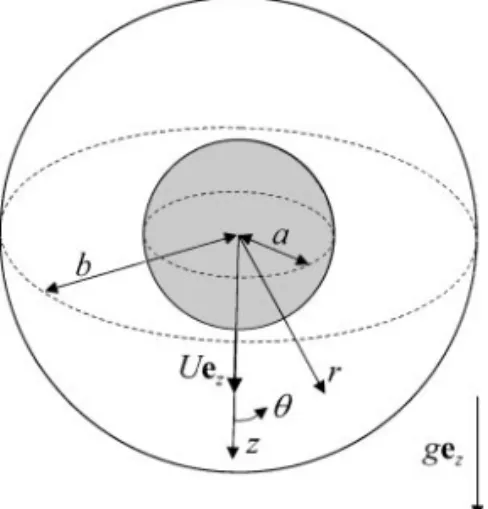
As shown in Fig. 1, we employ a unit cell model in which each particle of radius a is surrounded by a concentric spherical shell of suspending solution having an outer radius of b such that the particle/cell volume ratio is equal to the particle volume frac-tionϕ throughout the entire suspension; viz., ϕ = (a/b)3. The cell as a whole is electrically neutral. The origin of the spherical coordinate system (r, θ, φ) is taken at the center of the particle and the axisθ = 0 points toward the positive z direction. Obvi-ously, the problem for each cell is axially symmetric about the
FIG. 1. Geometrical sketch for the sedimentation of a spherical particle at the center of a spherical cell.
Conservation of all ionic species, which do not react with one another, requires that
∇ · Jm= 0, m = 1, 2, . . . , M, [1]
where Jm(r, θ) is the number flux distribution of species m. If
the solution is dilute, then the flux is given by
Jm= nmu− Dm µ ∇nm+ zmenm kT ∇ψ ¶ , [2]
where nm(r, θ), Dm, and zmare the concentration (number
den-sity) distribution, diffusion coefficient, and valence, respectively, of species m; u(r, θ) is the fluid velocity field relative to the parti-cle;ψ(r, θ) is the electric potential distribution; e is the elemen-tary electric charge; k is Boltzmann’s constant; T is the absolute temperature. The first term on the right-hand side of Eq. [2] represents the convection of the ionic species by the fluid mo-tion, and the second term denotes the diffusion and electrically induced migration of the species.
We assume that the Reynolds number of the fluid motion is vanishingly small, so the inertial effect on the fluid momentum balance can be neglected. The fluid flow is governed by the Stokes equations modified with the electrostatic effect,
η∇2u= ∇ p − ρge z+ M X m=1 zmenm∇ψ, [3] ∇ · u = 0, [4]
whereη and ρ are the viscosity and density, respectively, of the fluid, and p(r, θ) is the fluid pressure distribution.
The local electric potentialψ and the space charge density are related by Poisson’s equation,
∇2ψ = −4π ε M X m=1 zmenm. [5]
In this equation,ε = 4πε0εr, whereεris the relative permittivity of the electrolyte solution andε0is the permittivity of a vacuum. In Eqs. [2], [3], and [5], Dm, η, ρ, and εr are assumed to be constant in the fluid phase.
The boundary conditions at the surface of the dielectric par-ticle are as follows:
r = a, u = 0, [6a]
er· Jm= 0, [6b]
er· ∇ψ = −4π
ε σ, [6c]
where eris the unit normal outward from the particle surface and
σ is the surface charge density of the particle. In Eq. [6a], we
have assumed that the “shear plane” coincides with the particle surface. Equations [6b] and [6c] state that no ions can penetrate into the particle and the Gauss condition holds at the surface of the particle.
The boundary conditions at the virtual surface of the cell are as follows: r = b, ∂nm ∂r = 0, [7a] ∂ψ ∂r = 0, [7b] ur = −U cos θ, [7c] τrθ = η · r ∂ ∂r µ uθ r ¶ +1 r ∂ur ∂θ ¸ = 0
(for the Happel model), [7d] (∇ × u)φ = 1 r ∂ ∂r(r uθ)− 1 r ∂ur ∂θ = 0
(for the Kuwabara model), [7e] where ur and uθ are the r andθ components, respectively, of u. Note that the Happel cell model (12) assumes that the radial
velocity and the shear stress of the fluid on the outer boundary of the cell are zero, while the Kuwabara cell model (13) assumes that the radial velocity and the vorticity of the fluid are zero there. For the reason that the reference frame is taken to travel with the particle, the radial velocity given by Eq. [7c] is generated by the particle velocity in the opposite direction. The conditions [7c], [7a], and [7b] imply that there are no net flows of fluid, ionic species, and electric current between adjacent cells. They are valid because the suspension of the particles is bounded by impermeable, inert, and nonconducting walls. Thus, the effect of the backflow of fluid occurring in a closed container is included in both cell models.
Because the governing equations are coupled nonlinear partial differential equations, it is a formidable task for finding a general solution of them. Therefore, we shall assume that the system is only slightly distorted from the equilibrium state, where the par-ticle and fluid are at rest, and replace these nonlinear equations
by approximate linear equations. One can write
p= p(eq)+ δp, [8a]
nm= n(eq)m + δnm, [8b]
ψ = ψ(eq)+ δψ, [8c]
where p(eq)(r, θ), n(eq)m (r ), andψ(eq)(r ) are the equilibrium
dis-tributions of pressure, concentration of species m, and electric potential, respectively, andδp(r, θ), δnm(r, θ), and δψ(r, θ) are
the small perturbations to the equilibrium state. The equilib-rium concentration of any species is related to the equilibequilib-rium potential by the Boltzmann distribution,
n(eq)m = n∞m exp µ −zmeψ(eq) kT ¶ . [9]
Here, n∞m is the concentration of the type m ions in the bulk (electrically neutral) solution where the equilibrium potential is set equal to zero. Note thatψ(eq)and n(eq)
m depend on r only due
to spherical symmetry.
Substituting Eq. [8] into Eqs. [1], [3], and [5], canceling their equilibrium components, using Eq. [9], and neglecting the prod-ucts of the small quantities u,δnm, andδψ, one obtains
∇2δµ m= zme kT µ ∇ψ(eq)· ∇δµ m− kT Dm ∇ψ(eq)· u ¶ , m= 1, 2, . . . , M, [10] η∇2 u= ∇δp − ε 4π µ ∇2ψ(eq)∇δψ + ∇2δψ∇ψ(eq) ¶ , [11] ∇2δψ = −4π ε M X m=1 zmen∞m kT exp µ −zmeψ(eq) kT ¶ × (δµm− zmeδψ). [12]
Here,δµm is defined as a linear combination ofδnm andδψ
based on the concept of the electrochemical potential energy (6),
δµm=
kT n(eq)m
δnm+ zmeδψ. [13]
The conditions forδµmandδψ resulting from Eqs. [6] and
[7] and their equilibrium state are as follows:
r= a, ∂δµm ∂r = 0 and ∂δψ ∂r = 0, [14a,b] r= b, ∂δµm ∂r = 0 and ∂δψ ∂r = 0. [15a,b]
The fluid velocity u is a small perturbed quantity, and the bound-ary conditions for u have been given by Eqs. [6a], [7c], and [7d] or [7e]. In the analyses of Levine et al. (14) and Ohshima (15),
it was assumed that the overlap of adjacent double layers is neg-ligible on the virtual surface of the unit cell and Eq. [15] was replaced byδµm= 0 and δψ = 0 at r = b.
3. SOLUTION OF THE ELECTROKINETIC EQUATIONS FOR SYMMETRIC ELECTROLYTES
We now consider the sedimentation of a charged sphere in a unit cell filled with the solution of a symmetrically charged binary electrolyte with a constant bulk concentration n∞(M= 2, z+= −z−= Z, n∞+ = n∞− = n∞, where subscripts + and − refer to the cation and anion, respectively). The equilibrium elec-tric potentialψ(eq) satisfies the Poisson–Boltzmann equation, resulting from the substitution of the Boltzmann distribution [9] into Poisson’s equation [5], and the boundary conditions [6c] and [7b] at equilibrium. It can be shown that
ψ(eq)= ψ
eq1(r ) ¯σ + O( ¯σ3), [16] where ¯σ = 4π Zeσ/εκkT , which is the nondimensional surface charge density of the particle, and
ψeq1(r )= kT Z e µ κa A ¶ a r[(κb + 1) exp(κa + κr) + (κb − 1) exp(κa + 2κb − κr)], [17] with
A= (κb − 1)(κa + 1) exp(2κb) − (κa − 1)(κb + 1) exp(2κa).
[18]
Here, κ is the Debye–H¨uckel parameter defined by κ = (8π Z2e2n∞/εkT )1/2. Expression [16] forψ(eq)as a power se-ries in the surface charge density of the particle up to O( ¯σ ) is the equilibrium solution for the linearized Poisson–Boltzmann equation that is valid for small values of the electric potential (the Debye–H¨uckel approximation). That is, the surface charge density must be small enough for the potential to remain small. Note that, the contribution from the effect of O( ¯σ2) toψ(eq)in Eq. [16] disappears only for the case of symmetric electrolytes. To solve the small quantities u,δp, δµ±, and δψ in terms of the particle velocity U when the parameter ¯σ is small, these variables can be written as perturbation expansions in powers of ¯σ, u= u0+ u1σ + u¯ 2σ¯2+ · · · , [19a] δp = p0+ p1σ + p¯ 2σ¯2+ · · · , [19b] δµ± = µ0±+ µ1±σ + µ¯ 2±σ¯2+ · · · , [19c] δψ = ψ0+ ψ1σ + ψ¯ 2σ¯2+ · · · , [19d] U = U0+ U1σ + U¯ 2σ¯2+ · · · , [19e] where the functions ui, pi,µi±,ψi, and Ui are independent of
¯
σ. Both µ0± andψ0 must equal zero due to not imposing the concentration gradient and electric field.
Substituting the expansions given by Eq. [19] andψ(eq)given by Eq. [16] into the governing Eqs. [4] and [10]–[12] and bound-ary conditions [6a], [7c], [7d] or [7e], [14], and [15], and equat-ing like powers of ¯σ on both sides of the respective equations, we obtain a group of linear differential equations and boundary conditions for each set of the functions ui, pi, µi±, andψiwith
i equal to 0, 1, 2, . . .. These perturbation equations and their
so-lutions are presented in the Appendix, and the results for the r andθ components of u, δp (to the order of ¯σ2), δµ±, andδψ [to the order of ¯σ, which will be sufficient for the calculation of the sedimentation velocity and potential to O( ¯σ2)] can be written as ur = {U0F0r(r )+ U1F0r(r ) ¯σ + [U0F2r(r ) + U2F0r(r )] ¯σ2+ O( ¯σ3)} cos θ, [20a] uθ = {U0F0θ(r )+ U1F0θ(r ) ¯σ + [U0F2θ(r ) + U2F0θ(r )] ¯σ2+ O( ¯σ3)} sin θ, [20b] δp = η a{U0Fp0(r )+ U1Fp0(r ) ¯σ + [U0Fp2(r ) + U2Fp0(r )+ U0 εκ2a 4πηψeq1(r )Fψ1(r )] ¯σ 2 + O( ¯σ3)} cos θ, [20c] δµ± = Ze[U0F1±(r ) ¯σ + O( ¯σ2)] cosθ, [21] δψ = [U0Fψ1(r ) ¯σ + O( ¯σ2)] cosθ. [22] Here, functionψeq1(r ) has been given by Eq. [17], and func-tions Fir(r ), Fiθ(r ), Fpi(r ) (with i equal to 0 and 2), F1±(r ), and
Fψ1(r ) are defined by Eqs. [A4], [A14], [A15], and [A21] in the Appendix.
4. SEDIMENTATION VELOCITY
The total force exerted on the charged sphere settling in the electrolyte solution within a unit cell can be expressed as the sum of the gravitational force (and buoyant force), the electric force, and the hydrodynamic drag force acting on the particle. The gravitational force is given by
Fg= 4 3πa
3(ρ
p− ρ) gez, [23]
whereρpis the density of the particle.
Since the net charge within a unit cell is zero, the electric force acting on the charged sphere can be represented by the integral of the electrostatic force density over the fluid volume in the cell. Due to the fact that the net electric force acting on the particle at the equilibrium state is zero, the leading order of
the electric force is given by
Fe= − ε 2 Z π 0 Z b a ¡
∇δψ∇2ψ(eq)+ ∇ψ(eq)∇2δψ¢r2sinθ dr dθ. [24] Substituting Eqs. [16] and [22] into Eq. [24], one obtains
Fe=
½εκ2 6 [2a
2
Fψ1(a)ψeq1(a)− 2b2Fψ1(b)ψeq1(b)
+ G2(b)]U0σ¯2+ O( ¯σ3) ¾ ez, [25] where Gn(x)= Z x a rn[F1+(r )− F1−(r )] dψeq1 dr dr. [26]
The hydrodynamic drag force acting on the colloidal sphere is given by the integral of the fluid pressure and viscous stress on the particle surface,
Fh= 2πa2
Z π
0
{−δper+ η[∇u + (∇u)T]· er} sin θ dθ. [27]
Substitution of Eq. [20] into the above equation results in
Fh= − ½ 4πηaC02U0+4πηaC02U1σ +¯ · 4πηa(C22U0+ C02U2) +ε(κa)2
3 U0ψeq1(a)Fψ1(a)
¸
¯
σ2+ O( ¯σ3)
¾
ez, [28]
where coefficients C02 and C22 are given by Eqs. [A5b] and [A22b] for the Happel cell model and by Eqs. [A6b] and [A24b] for the Kuwabara cell model.
At the steady state, the total force acting on the settling particle (or the unit cell) is zero. Using this constraint after the addition of Eqs. [23], [25], and [28] for a symmetric electrolyte, one obtains the sedimentation velocity of the charged sphere in the expansion form of Eq. [19e] with the first three coefficients as
U0 = a2(ρ p− ρ)g 3ηC02 , [29a] U1 = 0, [29b] U2 = U0 C02 · −C22− εκ2b2 12πηaψeq1(b)Fψ1(b)+ εκ2 24πηaG2(b) ¸ . [29c]
Here, U0 is the settling velocity of an uncharged sphere in the cell, b= aϕ−1/3, and C02is a function of parameterϕ only and equals32asϕ = 0. The definite integrals Gn(b) in the closed-form
numerically. Note that the correction for the effect of surface charges to the particle velocity starts from the second-orderσ2, instead of the first-orderσ. The reason is that this effect is due to the interaction between the particle charges and the local induced sedimentation potential gradient; both are of orderσ, and thus the correction is of orderσ2.
Using Eqs. [16]–[18], one obtains a relation between the sur-face potential and the sursur-face charge density of the dielectric sphere at equilibrium,
σ = εζ
4πa
γ cosh γ + (κaγ + κ2a2− 1) sinh γ
(κa + γ ) cosh γ − sinh γ , [30] whereζ = ψ(eq)(a), which is known as the zeta potential of the particle, andγ = κa(ϕ−1/3− 1). Substitution of Eqs. [29] and [30] into Eq. [19e] results in an expression for the sedimentation velocity as a perturbation expansion in powers ofζ ,
U= U0 · 1− Hεζ 2 8πη µ 1 D+ + 1 D− ¶ + O(ζ3 ) ¸ , [31]
where the dimensionless coefficient H is a function of parame-tersκa and ϕ only,
H = −U2 U0
½γ cosh γ + (κaγ + κ2a2− 1) sinh γ κa[(κa + γ ) cosh γ − sinh γ ]
¾2 8πη ε × µ Z e kT ¶2µ 1 D+ + 1 D− ¶−1 , [32]
and its numerical result calculated by using Eqs. [29a] and [29c] will be presented in Section 6.
5. SEDIMENTATION POTENTIAL
The electric fields around the individual dielectric particles undergoing sedimentation in a suspension superimpose to give a sedimentation field ESED. For a homogeneous suspension of identical spherical particles, ESED is uniform and can be re-garded as the average of the gradient of electric potential over a sufficiently large volume V of the suspension to contain many particles. Namely, ESED= − 1 V Z V ∇δψ dV, [33]
where we have used Eq. [8c] and the fact that the volume average of the gradient of the equilibrium electric potential is zero. In order to calculate ESEDwe use the requirement that there exists no net electric current in the suspension. That is, the volume-average current density,
hii = 1
V
Z V
i(x) d V, [34]
must be zero. In Eq. [34], i(x) is the current density at position
x. The mathematical analysis given below is a modification of
that developed by O’Brien (21) and Ohshima et al. (6), in which the interaction between adjacent particles was not incorporated. For a solution containing M ionic species, the current density
i can be written as i= M X m=1 zmeJm. [35]
Substituting Eqs. [2], [8], and [13] into the above equation and neglecting products of the small perturbation quantities, one has
i= M X m=1 zmen(eq)m µ u− Dm kT ∇δµm ¶ . [36]
If the current density distribution reduced from the above equa-tion by taking n(eq)m = n∞m and∇ψ
(eq)= 0 (valid in the bulk so-lution beyond the double layers),
− M X m=1 zme Dm µ ∇δnm+ zmen∞m kT ∇δψ ¶ ,
is added and subtracted in the integrand of Eq. [34], one obtains
hii = − M X m=1 zme Dm V Z V µ ∇δnm+ zmen∞m kT ∇δψ ¶ d V + 1 V Z V " i+ M X m=1 zme Dm µ ∇δnm+ zmen∞m kT ∇δψ ¶# d V. [37]
In a statistically homogenous suspension with constant bulk ionic concentrations, the volume average of ∇δnm is zero.
According to the definition of Eq. [33] the first term on the right-hand side of Eq. [37] can be written as3∞ESED, where 3∞=PM
m=1z
2
me
2n∞
mDm/kT , which is the electric
conductiv-ity of the electrolyte solution in the absence of the particles. The integral in the second term on the right-hand side of Eq. [37] can be calculated by first considering for a single nonconduct-ing particle at the center of a unit cell and then multiplynonconduct-ing the result by the particle number N in V . Also, the volume integral for a cell can be transformed into a surface integral over the outer boundary of the cell. Thus, the second term becomes
N V Z r=b " n· ir + M X m=1 zme Dm µ δnm+ zmen∞m kT δψ ¶ n # d S = −N V M X m=1 zme Z r=b · r µ −n(eq) m u+ Dmn (eq) m kT ∇δµm ¶ · n − Dm µ δnm+ zmen∞m kT δψ ¶ n ¸ d S, [38]
where r is the position vector relative to the particle center and V/N = 4πb3/3. To obtain Eq. [38], the requirement of the conservation of electric charges (∇ · i = 0) and Eq. [36] have been used. In Ohshima’s analysis (15), the effect of overlapping double layers was neglected on the virtual surface of the cell (i.e., n(eq)m = n∞m was taken at r= b), so that the term involving
the fluid velocity u in Eq. [38] disappeared.
For a symmetric electrolyte with the absolute value of valence
Z , the average current density is obtained by the substitution of
Eq. [38] into Eq. [37] and the use of [7a], [7b], [13], [19], and [21], hii = 3∞E SED− Z en∞N kT V × ½ Z r=b ½ [2Z eψeq1(r )u0· r + D−µ1−− D+µ1+] ¯σ − (D+− D−)Z 2e2 kT ψeq1(r )ψ1σ¯ 2 ¾ n d S+ O( ¯σ3) ¾ . [39]
By the use of Eqs. [A3a], [A12], and [A13] and the requirement thathii = 0, the above equation yields
ESED=
4πb2Z2e2n∞N 3kT V3∞ U0
× {[2bψeq1(b)F0r(b)+ D−F1−(b)− D+F1+(b)] ¯σ
− (D+− D−)kTZ eψeq1(b)Fψ1(b) ¯σ2+ O( ¯σ3)}ez. [40]
Substituting Eqs. [17], [29a], [A4a], and [A14] into Eq. [40], and making relevant calculations, we can obtain the sedimenta-tion potential field in a suspension of identical charged spheres in the form
ESED= −
σa(ρp− ρ)g
η3∞ ϕEσ∗ez+ O(σ2). [41]
When the Happel cell model is used, the normalized sedimen-tation potential E∗σis Eσ∗ = 1 6 A(1− ϕ)¡2ϕ5/3+ 3¢ · eκa(1+ϕ−1/3)κa(8κ2a2ϕ2 − 18κ2a2ϕ5/3− 20ϕ5/3+ 2κ2a2ϕ + 40ϕ2/3 +1 2κ 4a4ϕ1/3+ 12κ2a2ϕ1/3− 12κ2a2− 24) + e2κa¡κaϕ−1/3+ 1¢µM+ N + K Z aϕ−1/3 a eκ(r−a) r dr ¶ + e2κaϕ−1/3¡κaϕ−1/3− 1¢ × µ M− N + K Z aϕ−1/3 a e−κ(r−a) r dr ¶¸ , [42] with M = ϕ5/3 µ κ2a2− 12 − 60 κ2a2 ¶ −1 8κ 4a4+3 4κ 2a2+ 12, [43a] N = ϕ5/3 µ κ3a3+ 2κa + 60 κa ¶ −1 8κ 5a5+5 4κ 3a3, [43b] K = 1 8κ 4a4¡8ϕ5/3− κ2a2+ 12¢. [43c] When the Kuwabara cell model is used,
E∗σ = 1 6 A(1− ϕ) · eκa(1+ϕ−1/3)κa µ 8 15κ 2a2ϕ2− 1 15κ 4a4ϕ4/3 −10 3 κ 2a2ϕ −4 5ϕ + 1 6κ 4a4ϕ1/3+26 5 κ 2a2ϕ1/3−4κ2a2 ¶ + e2κa¡κaϕ−1/3+ 1¢µM0+ N0+ K0 Z aϕ−1/3 a eκ(r−a) r dr ¶ + e2κaϕ−1/3¡κaϕ−1/3− 1¢ × µ M0− N0+ K0 Z aϕ−1/3 a e−κ(r−a) r dr ¶¸ , [44] with M0= 1 60ϕ µ κ4a4+ 6κ2a2− 240 − 720 κ2a2 ¶ − 1 24κ 4a4+1 4κ 2a2+ 4, [45a] N0= 1 60ϕ µ κ5a5+ 2κ3a3− 24κa +720 κa ¶ − 1 24κ 5a5+ 5 12κ 3a3, [45b] K0= 1 120κ 4a4(2κ2a2ϕ − 5κ2a2+ 60). [45c] Here, ϕ = (a/b)3= 4πa3N/3V is the volume fraction of the particles and the coefficient A has been defined by Eq. [18]. Note that Eσ∗ is a function of parametersκa and ϕ only. The definite integrals in Eqs. [42] and [44] can be performed numeri-cally.
Substitution of Eq. [30] into Eq. [41] leads to an expression for ESEDas a function ofζ,
ESED= −
εζ(ρp− ρ)g 4πη3∞ ϕE
∗
where
Eζ∗ = Eσ∗γ cosh γ − (1 − κ
2a2− κaγ ) sinh γ
(κa + γ ) cosh γ − sinh γ . [47] The numerical results of the normalized sedimentation potential
Eζ∗ as a function of parametersκa and ϕ will be discussed in the next section. If the σ2 term in Eq. [41] or the ζ2 term in Eq. [46] is needed, it can be obtained by detailed calculations of Eq. [40]. Note that, in the limit ofϕ → 0, the σ2orζ2term vanishes.
6. RESULTS AND DISCUSSION
In this section, we first consider several limiting cases of the expressions [31] and [46] for the sedimentation velocity and sedimentation potential, respectively, in a suspension of charged spheres. The correctness of these expressions may be confirmed by examining some of these limiting cases for which analyti-cal solutions are already known. Then, numerianalyti-cal results of the general cases will be presented.
In the limit of an infinitely dilute suspension (ϕ = 0), Eqs. [32] and [47] reduce to
H = 1
12{e 2κa
[5E6(κa) − 3E4(κa)]2− 8eκa[E5(κa) − E3(κa)]
+ e2κa[7E
8(2κa) − 3E4(2κa) − 4E3(2κa)]}, [48]
Eζ∗= 1 − eκa[5E7(κa) − 2E5(κa)]. [49]
where Enis a function defined by
En(x)=
Z ∞
1
t−ne−xtdt. [50] These degenerated results are the same as those obtained by Ohshima et al. (6) for a single dielectric sphere in an unbounded electrolyte. Note that the coefficient Eζ∗ given by Eq. [49] is the same as that obtained by Henry (22) for the electro-phoretic mobility of a dielectric sphere (the Onsager relation). Equations [48] and [49] result in H= 0 and Eζ∗=23 asκa = 0, and H= 0 [it can be shown that H = (κa)−2− (111/8)(κa)−3+ (1231/8)(κa)−4+ O(κa)−5] and Eζ∗= 1 as κa → ∞.
Whenκa À 1, the parameter Eζ∗in Eq. [47] has the asymptotic form Eζ∗= 3 ¡ 1− ϕ5/3¢ (1− ϕ)¡3+ 2ϕ5/3¢ − 3 1− ϕ(κa) −1+ O[(κa)−2]
(for the Happel model), [51a]
Eζ∗= 1 − 3
1− ϕ(κa)
−1+ O[(κa)−2]
(for the Kuwabara model). [51b]
The leading terms in the above expansions are identical to the formulas derived by Levine and Neale (16) for the normalized electrophoretic mobility of a dielectric sphere withκa → ∞. Note that, when κa → ∞, the value of E∗ζ predicted by the Happel model can be as much as 14% greater (occurring at
ϕ ∼= 0.39) than that predicted by the Kuwabara model.
Whenκa ¿ 1, Eq. [47] can be expressed as
Eζ∗ =1 3 · 3+ 2ϕ−5/3 3+ 2ϕ5/3 ϕ 2/3− ϕ−2/3 ¸ ×£(κa)2+ ϕ−1/3(κa)3+ O(κa)4¤
(for the Happel model), [52a]
Eζ∗ = 2
45
£
5ϕ−1− 9ϕ−2/3+ 5 − ϕ¤
×£(κa)2+ ϕ−1/3(κa)3+ O(κa)4¤
(for the Kuwabara model). [52b]
As expected, Eq. [52] predicts that the sedimentation potential does not exist (ϕE∗ζ= 0) in the limit of ϕ = 0 and κa = 0, where the effect of electrostatic interaction between the particle and the surrounding counterions is negligible.
According to Eqs. [31] and [32], the sedimentation velocity of dielectric spheres in electrolyte solutions can be calculated to the orderζ2orσ2. Figure 2 shows plots of numerical results for the dimensionless coefficient H in Eq. [31] as a function of parametersκa and ϕ. The calculations are presented up to
ϕ = 0.74, which corresponds to the maximum attainable volume
fraction for a swarm of identical particles (16). It can be seen that
H is always a positive value, and thus the presence of the particle
charges reduces the magnitude of the sedimentation velocity for any volume fraction of particles in the suspension. For a given value ofϕ, the effect of the particle charges on the sedimentation velocity is maximal at some finite values ofκa and vanishes at very large and small values ofκa. The location of the maximum in H shifts to greaterκa as ϕ increases. On the other hand, for a specified value ofκa in the intermediate range about 0.3–30, H is not a monotonic function ofϕ and has a maximal value. The location of this maximum shifts to greaterϕ as κa increases. As expected, the difference in H between the Happel model and the Kuwabara model (which can be either positive or negative depending on the combination ofκa and ϕ) is negligible for a dilute suspension (with smallϕ) and becomes apparent when the value ofϕ is large.
In Fig. 3, the normalized sedimentation potential Eζ∗in sus-pensions of identical charged spheres calculated from Eq. [47] is plotted as a function of parametersκa and ϕ. It can be seen that the dimensionless coefficient Eζ∗, which is always positive, decreases monotonically with the decrease ofκa (or with the in-crease of the double-layer overlap) for a fixed value ofϕ. When
κa = 0, E∗
ζ=23 asϕ = 0 and Eζ∗= 0 for all finite values of ϕ. Thus, when the double layers are thick (κa ≤ 0.2), the particle concentration effect on the sedimentation potential is significant
FIG. 2. Plots of the dimensionless coefficient H in Eq. [31] for sedimenting spheres versus parametersκa and ϕ. The solid and dashed curves represent the calculations for the Happel and Kuwabara cell models, respectively.
even in fairly dilute suspensions. For concentrated suspensions, this effect is evident for even relatively thin double layers (up to
κa ∼= 10). For the case of the Kuwabara model, E∗
ζ is a monotonic
decreasing function ofϕ for a constant value of κa and equals unity asκa → ∞ (regardless of the value of ϕ). For the case of the Happel model, however, Eζ∗is not a monotonic function of
ϕ and has a maximal value for a given value of κa greater than
about unity. The location of this maximum shifts to greaterϕ as
κa increases. For a fixed value of κa less than 1, this E∗
ζ is still
a monotonic decreasing function ofϕ. Figure 3 illustrates that, for any combination ofκa and ϕ, the Kuwabara model predicts a smaller value of Eζ∗(or a stronger concentration dependence of sedimentation potential) than the Happel model does. This occurs because the zero-vorticity model yields larger energy dissipation in the cell than that due to particle drag alone, owing to the additional work done by the stresses at the outer boundary (11).
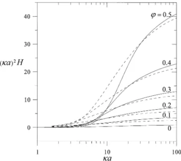
In the previous analyses for the sedimentation velocity and potential in suspensions of charged particles, it was assumed that the overlap of the double layers of adjacent particles could be neglected (14, 15). It would be of interest to know whether this assumption is valid at various situations. Comparisons of the results of the dimensionless coefficients (κa)2H andϕE∗
ζ
obtained in these previous analyses with our calculations relax-ing this assumption are presented in Figs. 4 and 5, respectively. It can be seen that, for a given value ofϕ, the analyses with non-overlapping double layers underestimate the coefficient H when
κa is large, overestimate H when κa is relatively small, and
un-derestimate the coefficient Eζ∗for an arbitrary value ofκa. The errors in the sedimentation velocity and sedimentation potential in suspensions owing to neglect of the effects of overlapping double layers of adjacent particles can be quite significant under typical conditions (even when the double layers are thin relative to the radius of particles).
FIG. 3. Plots of the dimensionless coefficient Eζ∗in Eq. [46] for a suspension of identical spheres versus parametersκa and ϕ. The solid and dashed curves represent the calculations for the Happel and Kuwabara cell models, respectively.
FIG. 4. Plot of the dimensionless coefficient (κa)2H for sedimenting spheres versusκa at fixed values of ϕ calculated for the Kuwabara cell model. The dashed curves represent the calculations performed by Levine et al. (14) neglecting the overlap of the electric double layers.
7. SUMMARY
In this paper, the steady-state sedimentation phenomena in homogeneous suspensions of identical charged spheres in electrolyte solutions with arbitrary value of κa are analyzed by employing the Happel and Kuwabara cell models. Solving the linearized continuity equations of ions, Poisson–Boltzmann equation, and modified Stokes equations applicable to the sys-tem of a sphere in a unit cell by a regular perturbation method, we have obtained the ion concentration (or electrochemical
po-FIG. 5. Plot of the dimensionless coefficientϕEζ∗for a suspension of iden-tical spheres versusϕ at fixed values of κa calculated for the Kuwabara cell model. The dashed curves represent the results given by Levine et al. (14) and Ohshima (15) neglecting the overlap of the electric double layers.
tential energy) distributions, the electric potential profile, and the fluid flow field. Since the electric potential distribution dif-fers from the equilibrium values, an electric force acting on the charged particle is induced. The total force exerted on the particle is the sum of the gravitational, electrostatic, and hydro-dynamic forces, and the requirement that the total force is zero leads to an explicit formula, Eq. [31], for the settling velocity of the charged spheres. The correction for the effect of the particle charges to the settling velocity begins at the second orderσ2or
ζ2. Numerical results indicate that this effect has a maximum at some finite values ofκa and disappears when κa approaches zero and infinity. The analytical expression for the average elec-tric current density in a suspension of identical spheres is given by Eq. [39]. The explicit formulas, Eqs. [41] and [46], for the sedimentation potential are derived from Eq. [39] by letting the net current in the suspension be zero. It is found that the di-mensionless sedimentation potential is a monotonic increasing function ofκa for constant values of the volume fraction of par-ticles. Comparisons of the results between the Happel model and the Kuwabara model have been provided. Also, our results show that the previous analyses for the sedimentation veloc-ity and potential in suspensions of charged particles with non-overlapping double layers can be in significant error at various situations.
Equations [31] and [46] with Eqs. [32] and [47] are obtained on the basis of the Debye–H¨uckel approximation for the equi-librium potential distribution around the dielectric sphere in a unit cell. The reduced formula of Eq. [32] for the sedimenta-tion velocity of a charged sphere with low zeta potential in an unbounded electrolyte solution, Eq. [48], was shown to give an excellent approximation for the case of reasonably high zeta po-tential (with an error less than 0.1% forζe/kT ≤ 2 in a KCl solution) (6). Therefore, our results might be used tentatively for the situation of reasonably high electric potentials. In or-der to see whether our approximate solution can be extended to the higher values of electric potential, a numerical solution of the electrokinetic equations with no assumption on the magni-tude of electric potential would be needed to compare it with the approximate solution.
APPENDIX: PERTURBATION EQUATIONS AND SOLUTIONS FOR THE MOTION OF A CHARGED
SPHERE IN A UNIT CELL FILLED WITH A SYMMETRIC ELECTROLYTE
After substituting the perturbation expansions given by Eq. [19] and the equilibrium distributions given by Eqs. [9] and [16] into Eqs. [6], [7], [10], [11], [12], [14], and [15], and equat-ing like powers of ¯σ on both sides of the respective equations, a set of differential equations and boundary conditions for each set of the functions ui, pi, µi±, andψi with i equal to 0, 1, and
Zeroth-Order Perturbations
Collecting the zeroth-order terms in the procedure of this reg-ular perturbation gives
∇2u 0=
1
η∇ p0, ∇ · u0= 0, [A1a,b]
u0|r=a = 0, u0r|r=b= −U0cosθ, [A2a,b] τ0rθ|r=b= 0 (for the Happel model), [A2c]
(∇ × u0)φ|r=b = 0 (for the Kuwabara model). [A2d]
The solution for the r andθ components of the velocity u0and the pressure p0satisfying the above equations is
u0r = U0F0r(r ) cosθ, [A3a] u0θ = U0F0θ(r ) sinθ, [A3b] p0 = η aU0Fp0(r ) cosθ, [A3c] where F0r(r )= C01+ C02 µ a r ¶ + C03 µ a r ¶3 + C04 µ r a ¶2 , [A4a] F0θ(r )= −C01− C02 2 µ a r ¶ +C03 2 µ a r ¶3 − 2C04 µ r a ¶2 , [A4b] Fp0(r )= C02 µ a r ¶2 + 10C04 µ r a ¶ . [A4c] In Eq. [A4], C01= − µ 1+3 2ϕ 5/3 ¶ ω, C02= µ 3 2+ ϕ 5/3 ¶ ω, [A5a,b] C03 = − 1 2ω, C04= 1 2ϕ 5/3ω, [A5c,d] for the Happel model, and
C01= − µ 1+1 2ϕ ¶ ω0, C 02= 3 2ω 0, [A6a,b] C03 = − µ 1 2 − 1 5ϕ ¶ ω0, C 04= 3 10ϕω 0, [A6c,d]
for the Kuwabara model, where
ω = µ 1−3 2ϕ 1/3+3 2ϕ 5/3− ϕ2 ¶−1 , [A7a] ω0=µ1−9 5ϕ 1/3+ ϕ −1 5ϕ 2 ¶−1 . [A7b] First-Order Perturbations
After collecting the first-order terms in the perturbation pro-cedure and using Eq. [A3a], one obtains
∇2µ 1±= ∓ Z e D±U0F0r(r ) dψeq1 dr cosθ, [A8] ∇2ψ 1− κ2ψ1= − κ2 2Z e(µ1+− µ1−), [A9] ∂µ1± ∂r ¯¯ ¯¯ r=a,b = 0, ∂ψ1 ∂r ¯¯ ¯¯ r=a,b = 0, [A10a,b] and the governing equations and boundary conditions for the flow field (u1, p1) are also given by Eqs. [A1] and [A2] with the subscript 0 being replaced by 1. The solutions for the r andθ components of u1, p1,µ1±, andψ1are
u1r = U1F0r(r ) cosθ, [A11a]
u1θ = U1F0θ(r ) sinθ, [A11b]
p1= η
aU1Fp0(r ) cosθ, [A11c]
µ1±= ZeU0F1±(r ) cosθ, [A12]
ψ1= U0Fψ1(r ) cosθ, [A13] where F1±(r )= ± 1 6D±(1− ϕ)r2 ½ a3Aµ(a, b) + 2ϕBµ(a, b) + 2r3 · ϕ Aµ(a, b) + b23Bµ(a, b) ¸ + 2(1 − ϕ)[Bµ(a, r) + r3Aµ(r, b)] ¾ , [A14]
Fψ1(r )= e2κa[2+ κa(κa − 2)]W{Aψ(a, b)e2κb[2+ κb(κb
− 2)] + Bψ(a, b)[2 + κb(κb + 2)]}
µκr + 1
r2
e−κr
+ [2 + κb(κb + 2)]W{Aψ(a, b)e2κa[2+ κa(κa − 2)] + Bψ(a, b)[2 + κa(κa + 2)]} µ κr − 1 r2 ¶ eκr + µκr + 1 r2 ¶ e−κrBψ(a, r) + µκr − 1 r2 ¶ eκrAψ(r, b). [A15]
In Eqs. [A14] and [A15],
Aµ(x, y) = Z y x F0r(r ) dψeq1 dr dr, [A16a]
Bµ(x, y) = Z y x r3F0r(r ) dψeq1 dr dr, [A16b] Aψ(x, y) = Z y x κr + 1 4κ e −κr[F 1+(r )− F1−(r )] dr, [A17a] Bψ(x, y) = Z y x κr − 1 4κ e κr[F 1+(r )− F1−(r )] dr, [A17b] W = {e2κb[2+ κa(κa + 2)][2 + κb(κb − 2)]
− e2κa[2+ κa(κa − 2)][2 + κb(κb + 2)]}−1. [A18]
Second-Order Perturbations
Among the second-order terms in the perturbation procedure, the only distributions we need in the calculations in Sections 4 and 5 for the sedimentation velocity and potential to O( ¯σ2) are the velocity u2and pressure p2. The equations governing u2and
p2are ∇2 u2= 1 η∇ p2− ε 4πη[∇ 2ψ eq1(r )∇ψ1+ ∇2ψ1∇ψeq1(r )], [A19a] ∇ · u2= 0. [A19b]
The boundary conditions for u2are also given by Eq. [A2] with the subscript 0 being replaced by 2. The solutions for the second-order perturbations of the components of u2and p2are
u2r = [U0F2r(r )+ U2F0r(r )] cosθ, [A20a] u2θ = [U0F2θ(r )+ U2F0θ(r )] sinθ, [A20b] p2 = · η aU0Fp2(r )+ η aU2Fp0(r ) +εκ2 4πU0Fψ1(r )ψeq1(r ) ¸ cosθ, [A20c] where F0r(r ), F0θ(r ), Fp0(r ), Fψ1(r ), andψeq1(r ) are given by Eqs. [A4], [A15], and [17], and
F2r(r )= C21+ C22 µ a r ¶ + C23 µ a r ¶3 + C24 µ r a ¶2 + εκ2 24πη × · G1(r )− 1 rG2(r )+ 1 5r3G4(r )− r2 5G−1(r ) ¸ , [A21a] F2θ(r )= −C21− C22 2 µ a r ¶ +C23 2 µ a r ¶3 − 2C24 µ r a ¶2 + εκ2 12πη · −1 2G1(r )+ 1 4rG2(r ) + 1 20r3G4(r )+ r2 5G−1(r ) ¸ , [A21b] Fp2(r )= C22 µ a r ¶2 + 10C24 µ r a ¶ +εκ2a 12πη · − 1 2r2G2(r )− rG−1(r ) ¸ . [A21c]
In Eq. [A21], Gn(x) is defined by Eq. [26],
C21 = − ·µ 1+3 2ϕ 5/3 ¶ A2+ 5 2ϕB2 ¸ ω, [A22a] C22 = ·µ 3 2 + ϕ 5/3 ¶ A2+ 5 2ϕ 2/3B 2 ¸ ω, [A22b] C23 = − · 1 2A2+ µ 3 2ϕ 2/3− ϕ ¶ B2 ¸ ω, [A22c] C24 = · 1 2ϕ 5/3A 2− µ ϕ2/3−3 2ϕ ¶ B2 ¸ ω, [A22d] A2 = εκ 2 24πη · G1(b)− 1 bG2(b) ¸ , [A23a] B2 = εκ2 120πη · 1 b3G4(b)− b 2G −1(b) ¸ , [A23b] for the Happel model, and
C21 = − ·µ 1+1 2ϕ ¶ A02+ µ 1−5 2ϕ + 3 2ϕ 5/3 ¶ B20 ¸ ω0, [A24a] C22 = · 3 2A 0 2+ µ 3 2 − 5 2ϕ 2/3+ ϕ5/3 ¶ B20 ¸ ω0, [A24b] C23 = − ·µ 1 2 − 1 5ϕ ¶ A02+ µ 1 2 − 3 2ϕ 2/3+ ϕ ¶ B20 ¸ ω0, [A24c] C24 = · 3 10ϕ A 0 2+ µ ϕ2/3−3 2ϕ + 1 2ϕ 5/3 ¶ B20 ¸ ω0, [A24d] A02 = εκ 2 24πη · G1(b)− 1 bG2(b)+ 1 5b3G4(b)− b2 5 G−1(b) ¸ , [A25a] B20 = εκ 2 120πη · −1 bG2(b)+ b 2G −1(b) ¸ , [A25b]
for the Kuwabara model, where ω and ω0 are defined by Eq. [A7].
ACKNOWLEDGMENT
This research was partially supported by the National Science Council of the Republic of China.
REFERENCES
1. Booth, F., J. Chem. Phys. 22, 1956 (1954).
2. Saville, D. A., Adv. Colloid Interface Sci. 16, 267 (1982). 3. Stigter, D., J. Phys. Chem. 84, 2758 (1980).
4. Wiersema, P. H., Leob, A. L., and Overbeek, J. Th. G., J. Colloid Interface
Sci. 22, 78 (1966).
5. de Groot, S. R., Mazur, P., and Overbeek, J. Th. G., J. Chem. Phys. 20, 1825 (1952).
6. Ohshima, H., Healy, T. W., White, L. R., and O’Brien, R. W., J. Chem. Soc.,
Faraday Trans. 2 80, 1299 (1984).
7. Liu, Y. C., and Keh, H. J., Colloids Surf. A 140, 245 (1998). 8. Keh, H. J., and Liu, Y. C., J. Colloid Interface Sci. 195, 169 (1997). 9. Stigter, D., J. Phys. Chem. 86, 3553 (1982).
10. Chen, S. B., and Koch, D. L., J. Colloid Interface Sci. 180, 466 (1996).
11. Happel, J., and Brenner, H., “Low Reynolds Number Hydrodynamics.” Nijhoff, Dordrecht, The Netherlands, 1983.
12. Happel, J., AIChE J. 4, 197 (1958).
13. Kuwabara, S., J. Phys. Soc. Jpn. 14, 527 (1959).
14. Levine, S., Neale, G., and Epstein, N., J. Colloid Interface Sci. 57, 424 (1976).
15. Ohshima, H., J. Colloid Interface Sci. 208, 295 (1998).
16. Levine, S., and Neal, G. H., J. Colloid Interface Sci. 47, 520 (1974). 17. Kozak, M. W., and Davis, E. J., J. Colloid Interface Sci. 127, 497 (1989). 18. Anderson, J. L., Ann. N.Y. Acad. Sci. 469 (Biochem. Eng. 4), 166 (1986). 19. Chen, S. B., and Keh, H. J., AIChE J. 34, 1075 (1988).
20. Zukoski, C. F., and Saville, D. A., J. Colloid Interface Sci. 115, 422 (1987).
21. O’Brien, R. W., J. Colloid Interface Sci. 81, 234 (1981). 22. Henry, D. C., Proc. R. Soc. London, A 133, 106 (1931).
![FIG. 3. Plots of the dimensionless coefficient E ζ ∗ in Eq. [46] for a suspension of identical spheres versus parameters κa and ϕ](https://thumb-ap.123doks.com/thumbv2/9libinfo/8844317.239975/9.918.501.860.446.1095/plots-dimensionless-coefficient-suspension-identical-spheres-versus-parameters.webp)