Parcel model for peak shapes in chromatography: Numerical verification of the temporal distortion effect to peak asymmetry

www.elsevier.com / locate / chroma

P

arcel model for peak shapes in chromatography

Numerical verification of the temporal distortion effect to peak

asymmetry

*

Su-Cheng Pai

Division of Marine Chemistry, Institute of Oceanography, National Taiwan University, P.O. Box 23-13, Taipei, Taiwan Received 5 November 2002; accepted 23 December 2002

Abstract

The traditional plate concept has been reassessed and improved to a parcel matrix model, which can be used to imitate the chromatographic behavior of a hypothetic column on a computer worksheet. Under programmed conditions, various peak shapes (nearly Gaussian, and with prolonged or fronting tails) are generated. The peak tailing has been separated into two major fractions: spatial and temporal. The former fraction is caused by the retention nature of a column, whereas the latter is induced by the observer’s relative position and the changing of the zone broadening rate. The temporal distortion effect can be identified qualitatively and quantitatively through a normalized peak-overlapping process. In general, a chromatographic peak may carry a prolonged (or normal type) tail under linear isotherms, while both prolonged and fronting tails will appear under non-linear conditions. The temporal distortion is proved to be significant, and may be regarded as the major cause of peak asymmetry in most cases. This is in contrast to the conclusions of many previous studies. The model is also eligible to simulate chromatographic peaks for various injection sizes.

 2003 Elsevier Science B.V. All rights reserved.

Keywords: Parcel model; Peak shape; Temporal distortion effect; Peak tailing

1

. Introduction Further discussion on the tailing phenomenon is

diverse among different communities. Most routine 1

.1. Peak shape problems analysts would regard the peak tailings as

malfunc-tions or artifacts of the instrumentation, and ignore it In analytical textbooks [1–3], the basic shape of a because it does not affect the quantification. The chromatographic peak is usually assumed to be plate numbers can still be estimated in an empirical ‘‘symmetrical’’ and can be approximated by a Gaus- way [4]. To simulate skewed peak shapes, several sian equation. In practice, the peak shapes may not equations (e.g. the exponentially modified Gaussian, always be symmetrical. Skewed peaks do occur EMG) have been suggested [5–7]. The results have frequently in the laboratory, either with prolonged been claimed to be successful and useful in solving (normal type) or fronting (reverse type) tails. overlapped peaks on a chromatogram, regardless of the fact that small residuals between the modeled and experimental peaks are always present.

*Tel.: 1886-2-2362-7358; fax: 1886-2-2363-2912.

E-mail address: [email protected](S.-C. Pai). Theorists have shown much more interest in the

0021-9673 / 03 / $ – see front matter  2003 Elsevier Science B.V. All rights reserved. doi:10.1016 / S0021-9673(03)00029-3

modeling of peak tails. Although some potential where s is the standard deviation of a sample zoneL

on the longitudinal coordinate (L axis), resulting sources that can cause peak deformation have been

from the accumulation of the initial zone width, the identified [8,9], explanations are somewhat vague

effect of mass diffusion, the effect of retention by the and difficult to understand. Peak asymmetry

prob-stationary phase, and other physical effects such as lems, especially peak fronting, remain puzzling.

non-equal path, extra-column, etc. By combining all It is deemed that something in the existing theories

mechanisms as a whole, the distribution can be might have been misinterpreted or overlooked. The

approximated as a peak function by taking the most possible suspect would be the ‘‘temporal

2 2

solution of Fick’s law (≠C / ≠t 5 D ≠ C / ≠L 2 u

distortion effect’’ [10]. If this effect has been proved x

≠C / ≠L, where D is the empirical diffusion

coeffi-to exist in a flow injection system, it must also occur

cient of the system, u the migration speed of an

in chromatography. x

analyte X ) to generate a Gaussian-type distribution curve or the concentration profile, C(L ), on the L 1

.2. The fractions of tailing

coordinate [11]:

A peak tail can comprise two major fractions: C Wo o 2(L 2u t ) / 2s_x 2 2_L

]]]

C(L ) 5 ] e (2)

spatial and temporal. In the past, the spatial fraction _{Œ2p s}

L

was considered exclusively responsible for the

tail-where C and W are the initial concentration and

ing. The focus has been on the uneven packing of o o

zone width of the injected sample; t the time

resin in a column, shapes of detector, tube wall _]

Œ

duration, and s 5 2Dt. The curve plotted for Eq.

friction effects, etc. The temporal fraction, on the L

(2) at a selected time is a Gaussian peak, which is contrary, has seldom been mentioned or discussed in

usually named the mass distribution pattern. the literature.

If this pattern is to be observed by a detector, the The temporal contribution to the peak tailing may

coordinate should be transferred to a time scale, i.e. be described by a concept of relativity [10]: when a

plotted for C(t) instead of C(L ). By treating L as a

shape-changing subject (symmetrical or not

constant and time a variable, the curve plotted for symmetrical) passes through a single fixed position

C(t) would turn from ‘‘symmetrical’’ to ‘‘not detector, the observer will receive a distorted pattern

symmetrical’’ [12,13]. A tail is generated, not in the from the real image of that subject at a specific time.

space domain, but in a time domain. It should be For column-type chromatography, the detector is

named the temporal tailing. usually located at the outlet of the column, which

In practice, it is still difficult to distinguish the two records signals when the sample zone passes

tailing fractions just from the peak appearance. through. If the zone broadening rate (ds / dt) in the

Although most analysts would prefer to solve the column is large, the resultant chromatographic peak

peak asymmetry problems directly from the diffusion will be distorted regardless of whether or not the

equations, it should be noted that the coefficient D in mass pattern is symmetrical. On the recorder, the

Eq. (2) comprises both diffusion and retention terms. temporal fraction of a tail is spatially false.

The diffusion effect is unlikely to cause a peak to be asymmetrical. On the contrary, it diminishes rather 1

.3. False tailing in diffusion models

than generates the asymmetry of a peak. Therefore the diffusion approach sometimes might cause the It is not difficult to find evidence of the false

problem to be more ambiguous. In this respect, the tailing fraction in previous diffusion models. In those

original plate concept [14,15], which focuses ‘‘only’’ models, the formation of a peak in a

chromato-on the retentichromato-on effect, is more straightforward and graphic column is considered as the ‘‘broadening’’ of

practical. the sample zone (in terms of peak width W or

standard deviation s) by a number of mechanisms 1

.4. False tailing in plate models [1,2]. Mathematically it can be expressed as:

2 2 2 2

sug-gested previously, including the dynamic plate model following isotherm (at a constant temperature): K 5 by Glueckauf [16] and the statistic plate model C /C , where K is the distribution constant, C ands m s

suggested by Fritz and Scott [17]. In those models, Cm are the concentrations of a substance in the the mass distribution patterns and the chromato- stationary and mobile phases, respectively. The graphic peaks (or the exit time curve), are all not equilibrium can also be described in a mass unit if symmetrical at initial stages or when the plate taking the volume factor to be constant:

number is small. However, those authors did not pay

k9 5 m /ms m (3)

too much attention to the peak asymmetry problem.

where k9 is the mass partition ratio between the two Their conclusions are made on the symmetrical side:

phases, which is frequently termed the capacity ratio the peak shape will soon turn to a Gaussian curve

of a substance in a column. when the plate number increases; the tailing will be

Since the complete partition equilibrium can insignificant and not important at large plate

num-‘‘never’’ be achieved, an apparent or dynamic parti-bers.

tion ratio k0 is introduced: Since the temporal distortion fraction has never

been separated and discussed individually, the author _{k0 5 d k9 (4)}

u

believes that it could be the key to the deciphering of

where d is the degree of completeness of the

the peak asymmetry puzzle. It is very possible that u

equilibrium (ranges 0–1) at a given flow speed u. It all types of peak tailings (prolonged or fronting)

may be described as an exponential function of the have already been endorsed in the plate concept, but

equilibrium time (t ) in a plate, which is a reciprocal

have yet to be interpreted appropriately. A detailed eq

function of the flow speed u. When the effluent flows reassessment on those plate models is deemed

neces-very slowly, d approaches 1 and k0¯ k9; whereas

sary. u

when the flow is at a fast speed, both d and k0 canu

be very small. 1

.5. Focus of this study

At constant flow speed, k0 can be influenced by temperature and the composition of the mobile The targets of the present study are to improve the

effluent. In many applications these conditions are plate model so that spatial and temporal tailing

programmed to change in order to obtain optimal fractions can be verified separately, and to exemplify

separations (e.g. the elevation of temperature for GC possible situations that may cause prolonged and

and the changing of effluent composition for HPLC). fronting peaks. In combination it is expected to

Under these non-linear conditions, the partition ratio provide analysts with a practical tool for simulating,

k0 becomes a variable with time and should be predicting and solving chromatographic peaks before

denoted as k0(t). and after commencing an experiment. The skills of

using a computer worksheet as suggested by de

Levie [18,19] were generally adopted, but expanded 2 .2. The parcel concept to include various isotherms. A ‘‘parcel’’ concept has

been proposed, which enables the contribution of the To advance the plate equilibrium continuously temporal distortion effect to be more clearly dis- along a column, Glueckauf [16] added a ‘‘time’’

played. label to each plate to show its location along the time

coordinate. To further expand the usage of this concept, the ‘‘time-labeled plate’’ has been regarded

2

. Theoretical as a ‘‘parcel’’ in this paper.

A parcel is defined as a unit section of a column at 2

.1. Equilibrium in a plate a particular moment. Allowing the column length L

to be separated into many small sections, L 5 nDL, In plate theory [14], a ‘‘plate’’ is a unit section or and the time duration t to be divided into many small layer of a narrow column. For partition chromatog- time steps, t 5 tDt, each parcel is denoted as P(n,t) raphy the equilibrium within a plate should obey the with a section number n and a time step number t.

The n 3 t parcel matrix imitates the entire column is decided by a diffusion coefficient D and the operation over the time duration, and a parcel is the gradients between parcel pairs, e.g. P(n 2 1,t 2 1) /

minimal fraction unit of this matrix. P(n,t 2 1) and P(n,t 2 1) /P(n 1 1,t 2 1).

The mean flow velocity (u) of the mobile effluent The total mass within a parcel P(n,t) is marked as is defined to be u 5 L /t 5 nDL /tDt, or u 5 n /t 3 mt(n, t ), and it can be split into the stationary and

DL /Dt. Since the calculation is made ‘‘section-by- mobile phases, i.e. ms(n, t ) and mm(n, t ), respectively, section’’ and ‘‘step-by-step’’, and n and t are all according to the dynamic equilibrium at a given time integers, a dimensionless flow velocity v is defined step:

to be 1 for the discrete calculation on the parcel

ms(n, t )

matrix. _{k0 t 5s d ]] (6)}

mm(n, t )

2

.3. Mass flux balance in a parcel

The total incoming mass is re-distributed into the two phases:

The complete mass balance for a given parcel

P(n,t) can be expressed in terms of mass fluxes (F ,i m 5 m 3 k0(t) / [k0(t) 1 1] (7)

s(n, t ) t(n, t )

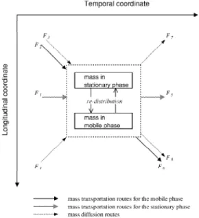
the mass changes per time step, see Fig. 1):

m 5 m / [k0(t) 1 1] (8)

Fincoming5 F 1 F 1 F 1 F 5 F1 2 3 4 output m(n, t ) t(n, t )

5 F 1 F 1 F 1 F5 6 7 8 (5)

After the equilibrium, the mass fluxes that leave the parcel P(n,t) are: F , the stationary fraction mass5

The total incoming flux for P(n,t) includes: F , the1

transported to P(n,t 1 1); F , part of the mobile6

stationary mass transported from P(n,t 2 1); F , the2

fraction mass transported to P(n 1 1,t 1 1); and F7

mobile mass transported from P(n 2 1,t 2 1); and F3

and F , part of the mobile-phase mass diffused to8

and F , the mass diffused from P(n 2 1,t 2 1) and4

P(n 1 1,t 1 1) and P(n 2 1,t 1 1), respectively. P(n 1 1,t 2 1). The magnitude of the diffusion flux

2

.4. Simplified parcel matrix

The reproduction of a single parcel to an n 3 t matrix gives a cross-linked structure, which indicates all possible mass transportation routes in the column operation. However, the calculation can be quite complex if the diffusion fluxes are included. As mentioned in Section 1.3, the addition of the diffu-sion terms does not really help an analyst to answer: ‘‘why is the peak shape not symmetrical?’’. For these reasons, the parcel matrix is simplified by deleting all diffusion fluxes and leaving only the transporta-tion routes for the statransporta-tionary and mobile phases (Fig. 2). However, it is still possible to add the diffusion effect later as a modification, after the basic peak shape has been generated (please note that a diffu-sion modification will make the peak slightly wider,

Fig. 1. Mass flux balance of a single parcel on the longitudinal–

but will not affect the trend of the skewness).

temporal dimensions. The total incoming mass received from the

Thus, the simplified mass balance for a parcel

left parcels (Fincoming5 F 1 F 1 F 1 F ) is re-distributed into1 2 3 4

P(n,t) becomes:

stationary and mobile phases, and they are delivered out to the parcels on the right (Foutput5 F 1 F 1 F 1 F );5 6 7 8 where

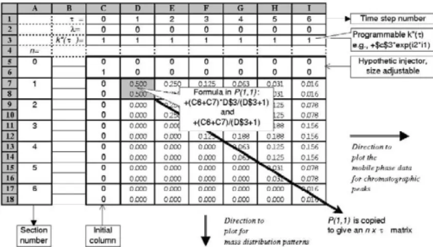
Fig. 2. A simplified longitudinal–temporal parcel matrix formed by cross-linking the transportation routes for the stationary and mobile phases and deleting (for clearance) the possible mass diffusion routes.

Accordingly, a ‘‘unit’’ parcel contains just two upper one for ms(n, t ) and the lower for mm(n, t ). The

calculation terms: unit parcel is copied both longitudinally (vertically

down) and temporally (horizontally right) to give an ms(n, t )5 [ms(n, t 21 )1 mm(n 21, t 21 )]k0(t) / [k0(t) 1 1] _{n 3 t matrix (see Fig. 3 for a 636 example).}

(10) Two additional parcel sets are also created. The parcel set from P(1,0) to P(n,0) imitates the initial state of the virtual column; and the other from P(0,0) mm(n, t )5 [ms(n, t 21 )1 mm(n 21, t 21 )] / [k0(t) 1 1]

to P(0,n) is reserved for the hypothetic injector. (11)

The same conditions apply to all parcels on the _{2 .6. Injection size} matrix. The directions of the calculation (delivery of

values) are horizontally for the stationary phase and _{The size of the injector on the matrix is usually}

diagonally for the mobile phase. _{unique, but can be optional and adjustable. For a}

single impulse injection, the injector occupies only one parcel at P(0,0). To double the sample size, it 2

.5. Parcel matrix on worksheet

occupies two parcels from P(0,0) to P(0,1). For frontal analysis or pre-concentration simulations in The parcel matrix can be displayed on a computer

which the sample is loaded continuously, the injector worksheet, e.g. Microsoft Excel. The recursion

treat-can be further expanded to the right end of the ment is quite similar to that suggested by de Levie

matrix. [18]. Each parcel occupies two worksheet cells, the

Fig. 3. Setting up of an n 3 t parcel matrix on the Microsoft Excel worksheet by copying the recursion equations within a unit parcel (e.g. in P(1,1)) along both coordinates. Each parcel occupies two worksheet cells (the upper for the stationary phase and the lower for the mobile phase). The hypothetic injector occupies a row of parcels from P(0,0) to P(0,t) depending on the sample size. If a single impulse is needed then a mass value is filled into the mobile phase cell of P(0,0). The redistribution equilibrium is governed by k0(t), which is variable with time step and can be programmed (in the 3rd row cells) to be consistent, stage-wise or continuous decreasing.

2

.7. Programmable k0(t) 2 .8. Operating the parcel matrix

The k0(t) value can be programmed, as either The procedures of operating the parcel matrix are consistent, stage-wise decreasing or continuous de- as follows.

creasing. For linear isotherms, the k0(t) values for all 1. Define the status of the isotherm by inputting a time steps are the same (filled all cells with the same value for the decay constant ( l). In linear cases, value). For stage-wise changing, different values can l 5 0.

99 99

be filled for several time step periods, e.g. k0(t) 5 k1 2. Input an initial ko value at t 50; then fill other

99

from t to t , k0(t) 5 k0 1 2 from t to t , . . . etc. In1 2 k0(t) cells with desired values or copy an equation many circumstances the changing of isotherm can be to the entire time step duration. In linear cases,

99

made continuously, either in a ‘‘direct’’ or ‘‘ex- k0(t) 5 k .o

ponential’’ relationship to the time step. For this, one 3. For a single impulse, fill a mass value for mm( 0,0 )

may choose either of the following equations and fill in P(0,0). If the injector occupies more than one into the corresponding cells on the worksheet: parcel, fill all other parcels with the same values. Once the injection has been done, the worksheet

99

k0(t) 5 k (1 2 lt)o 0 # lt # 1 (12) generates immediately two data (m and m ) fors m

each parcel and fills automatically the whole n 3

or, t parcel matrix.

4. Select a time t to view the mass distributions: the

2lt

99 data sets in the vertical parcel column P(n,t) are

k0(t) 5 k eo (13)

used for plotting three ‘‘mass distribution pro-where l is the decay constant. To simulate GC files’’ along the n coordinate, namely, the mass in operation the latter equation is much more prefer- the stationary phase, mobile phase, and total (sum able, as the dropping of k0(t) is in a reciprocal of both).

relationship to the temperature elevation rate (dT / 5. Select a longitudinal position to view the ‘‘elution dt). On the matrix, Eqs. (12) and (13) can also be profile’’ or ‘‘chromatogram’’. The chromato-written in recursion forms as: k0(t) 5 k0(t 2 1) 2 l graphic peak, if observed by a hypothetical and k0(t) 5 k0(t 2 1)(1 2 l), respectively. detector located at a position n 5 N, refers to the

mm(N, t ) data (mobile phase only) in the horizontal although the peak appears at t , its theoreticalr

parcel set P(N,t). The diagram is plotted along the standard deviation should still refer to the mass

t coordinate. position at t , and is estimated by:rm

6. If DL and Dt have been defined (e.g. DL 5 1 cm;

s (t ) ¯ s (t )(k0(t ) 1 1)t rm n rm rm (16)

Dt 5 1 s, or else), then the above dimensionless

plots can be transformed to L or t coordinates. _{3. On the matrix.}

• The migration speed (v (t)): the rate of longi-m

2

.9. Peak parameters on matrix _{tudinal movement of the mass center per time}

step, defined as: Following the above procedures, two types of

Dn (t)p 1

diagrams (spatial and temporal) can be generated. _{v (t) 5]]5]]] (17)}

m _{Dt k0(t) 1 1}

The definitions of the peak parameters are described

separately as follows. _{The highest migration speed is 1 when k0(t) 5}

1. Along the n coordinate, at a selected t. _{0, and becomes near zero when k0(t) is very}

• Mass peak heights (h , h , h ): the maximumt s m _large.

mass values (refer to total, stationary and _{• The migration route of the mass center (n (t)):}

p

mobile phases, respectively) that appear in a _{it is obtained by a recursion calculation on the}

vertical parcel set at a selected time step. _{parcel matrix:}

• Mass peak position (n ): the section numberp

n (t) 5 n (t 2 1) 1 Dn (18)

that contains the maximum mass values (mass p p p

maxima for the stationary and mobile phases

• The migration slope (or t /n ratio): a reciprocal are synchronized).

function of migration speed v (t), or t /n(t) 5

• Arrival time of the mass peak (t ): for a fixedrm m

k0(t) 1 1. column length, the total time step required for

• Peak locations: for a given column length N, the mass peak to arrive at the detector.

the migration route curve crosses the

horizon-• Band broadening rate: mathematically defined

tal n 5 N line at the parcel address P(N,t );

following the suggestion by Fritz and Scott rm

whereas the chromatographic peak is seen at [17]:

the address P(N,t ). The two addresses co-r

]]

Ds tns d

œ

]]5]]] (14)

Dt k0(t) 1 1

2

.10. Overlapping the spatial and temporal peaks

• Standard deviation of the sample zone (s (t)):n

on the worksheet, the recursion calculation

Although the mass pattern should never be ob-formula can be written as:

served by a single detector, it can be displayed

]]]]]_{2 2}

s (t) 5 s (t 2 1) 1 Dsn

_œ

• Peak width on n coordinate (W (t)): it isn

of the temporal distortion effect. defined as W (t) 5 4s (t).n n

However, the spatial and temporal peaks cannot be 2. Along the t coordinate, at a selected n.

plotted directly on the same coordinate, and a

• Chromatographic peak height (h ): the maxi-t

normalization process must be taken. The major mum value found in the ‘‘mobile phase cells’’

concerns are the mirror image effect due to the of the horizontal parcel set.

observing position, and the expanding effect due to

• Chromatographic peak position (t ): the equiv-r

the migration speed. To compensate for these effects, alent to the traditional ‘‘retention time’’ of a

the n coordinate should be firstly converted to 2N 2 peak that appears on the recorder chart. It does

n coordinate, and then multiplied by a factor not equal trm by definition.

k0(t ) 1 1.

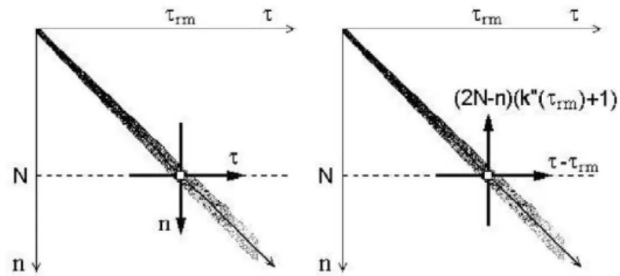
Fig. 4. Axial transformations for the overlapping of the spatial profile and temporal peak at the mapping center P(N,t ). Left, collectrm mobile-phase mass data along n and t coordinates. Right, re-plot data on the normalized (2N 2 n)(k0(t ) 1 1) and t 2 trm rmcoordinates, and then overlap the two diagrams.

The mapping procedures are suggested below peaks were plotted for detectors at n 55, 10, and 15,

(also see Fig. 4). respectively (Fig. 6).

Step 1 For a given column length N, locate the

address P(N,t ) as the mapping center forrm 3 .2. General aspects of the linear parcel model both peaks.

Step 2 Obtain ‘‘only’’ the mobile-phase mass val- Under linear isotherms, and if the sample size ues (together with their corresponding n or t injected is limited to a ‘‘single impulse’’, the present scaling values) along the vertical column parcel matrix model is no different from that

sug-and horizontal row. gested by de Levie [18,19]. It is also equivalent to

Step 3 Re-plot the vertical mass values on the (2N – the binominal equations that derived from a

statisti-n)(k0(t ) 1 1) coordinate.rm cal discrete plate model by Fritz and Scott [17].

Step 4 Re-plot the horizontal mass values on the Thus, the masses contained within a parcel at any

t 2 trm coordinate. given address P(n,t) can also be expressed as:

Step 5 Overlap the two re-plotted peaks on one 1. in stationary phase: diagram.

ms(n, t )

The difference (or the residual curve) between the

t 2n 11 n 21

(t 21)! k0 1

normalized spatial and temporal curves gives the

]]]] ]]

S

D

S

D

5mo

‘‘net’’ temporal distortion effect. (t 2n)!(n21)! k011 k011

(19) 2. in mobile phase:

3

. Numerical demonstration under linear

mm(n, t ) isotherms t 2n n (t 2 1)! k0 1 ]]]]] ]]

S

D S

D

.1. Demonstration of a single impulse injection

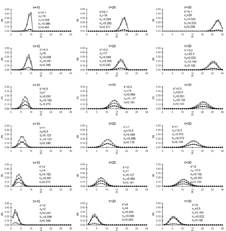
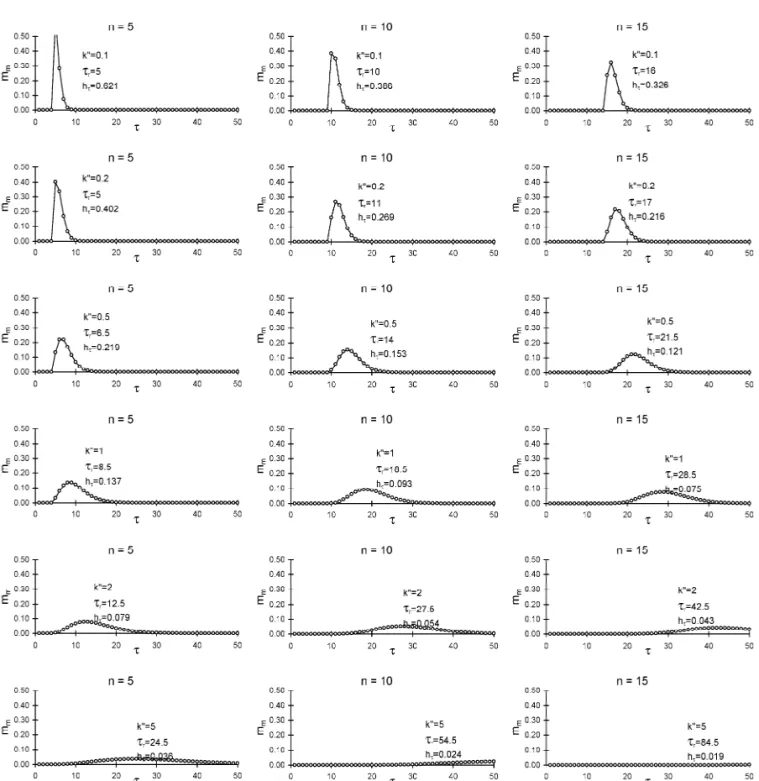
(20) A 30350 parcel matrix was found to be conveni- _{3. the total (sum of both phases):}

ent to illustrate the shape of a single peak under m linear isotherms, i.e. l50 and k0(t) 5 k0. In this t(n, t )

t 2n

section six k0 values (i.e. k0 5 0.1, 0.2, 0.5, 1, 2 and _{(t 2 1)! k0 1} n 21

]]]]] ]]

S

D S

D

5 m

5) were used. The injector occupied one parcel, and o_{(t 2 n)!(n 2 1)! k0 1 1 k0 1 1}

the injected mass number (m ) was 1. Mass dis-o

(21) tributions were examined at t 510, 20 and 30,

Fig. 5. Mass distribution patterns for the stationary phase (m , solid circle), mobile phase (m , open circle) and total (m 5 m 1 m , opens m t s m cube) along the n coordinate under linear isotherms. Data are calculated at t 510, 20 and 30, respectively, with various k0 values. The position of the mass center n as well as the corresponding heights for h , hp s mand h are also given to each mass peak.t

e.g. m (n) or m (n), along the n coordinate at at m Even though those authors have discussed the given t gives the mass distribution patterns. general features of the chromatographic peak shapes Plotting of Eq. (20) in the form m (t) along the tm previously, it is still worthwhile to re-examine the coordinate for a column length n 5 N gives the peak parameters in both spatial and temporal

3

.3. Mass profiles pands like a ridge on the matrix. The migration

speed is v 5 1 /(k0 1 1), and the t /n slope is k0 1 1.m

The mass profiles shown in Fig. 5 clearly indicate Ideally, for the single impulse injection, the migra-that they are influenced by both the k0 value and tion route should be described by n 5 v t. How-p m

observation time in terms of shape, position, as well ever, this is obeyed only when k0 5 0; a consistent as the peak height. For the single impulse injection, shift is found for those k0 . 0. For example, when the ‘‘k0 5 0’’ and ‘‘k0 5 1’’ are decisive boundaries k0 5 1, the mass maxima are found in the parcels of

controlling the skewness of a mass peak: P(1,1), P(1.5,2), P(2,3), P(4,7), P(6,11), P(10,

1. when k0 5 0, the mass will not enter the stationary 19), . . . etc., and the migration route becomes: phase at any time, and will appear at the void

n (t) 5 t /(k0 1 1) 1 0.5p (22)

position without shape-changing;

2. when 0 , k0 , 1 the mass distributes more in the

The 0.5 is named the ‘‘longitudinal shift’’, a practical mobile phase, and the migration speed is

rela-term for the parcel matrix. The shift is because the tively fast. The patterns for the mobile phase,

injected size is not zero but 1DL, therefore the initial stationary phase, as well as the sum of both, all

mass center is at the 10.5 position on the n look non-symmetrical. The skewness is more

coordinate. To show the peak position on a matrix, obvious when k0 is very small or near zero, the

the n value of Eq. (22) should be rounded off to thep

peaks lean slightly toward the right on the chart (a

nearest integer unless with a decimal value of exactly mirror image of a normal-type tailing), and the

0.5 (at which the mass center lies exactly between peak positions are close to the void position;

two parcels). For example, if t 520 and k0 5 0.1; the 3. when k0 5 1 the mass distributes evenly between

value for n (20) is 18.68 and the mass center willp

the stationary and mobile phases and the patterns

appear in parcel P(19,20); when k0 5 0.2, n (20) 5p

are completely symmetric over the entire time

17.17, the mass center will be in parcel P(17,20); duration;

when k0 5 1, n (20) 5 10.5, the mass center liesp

4. when k0 . 1, the situations invert to k0 , 1. More

between P(10,20) and P(11,20). mass fraction tends to stay in the stationary phase.

The time required for a mass center reaching the The peaks lean toward the left (a mirror image of

end of a column (length N ) is marked as t :rm

a fronting-type tailing) and the migration along

the column is relatively slow. _{t 5 (N 2 0.5)(k0 1 1) (23)}

rm

It is also found that the total mass curves for k0 5 0.2 and 5 are mirror images of each other, so as

When the column is long, the 0.5 shift may no for k0 5 0.5 and 2, and every k0 and 1 /k0 pairs. The

longer be important and the equation will appear difference would be that the proportions of the mass

similar to that found in textbooks. However, it in the stationary and mobile phases are reversed.

should be emphasized that trm should not be treated If the injector size were larger than one parcel, the

as the conventional retention time t for a chromato-r

general trends as stated above are still applicable;

graphic peak. only the patterns for k0 5 1 are no longer completely

Again, Eqs. (22) and (23) are valid for the single symmetrical in the starting stage.

impulse injection only. The increase of sample size will cause an extra delay for both n and t .p rm

3

.4. Position of mass peaks on the matrix

The location of the maximum mass values in the 3 .5. Zone broadening on the n coordinate vertical parcel set is the position of the mass peak. It

may not necessarily be found in a single parcel In principle, the broadening of a sample zone is a because sometimes the values for two adjacent function of the square root of time step number t, as parcels are identical. In this case a 0.5 unit is stated in Eq. (15). However, since the initial sample employed to address the peak position. zone on the matrix is not zero, an initial s (0) valuen

Fig. 6. Chromatographic peaks (with various k0) observed at positions n 55, 10 and 15, respectively, under linear isotherms. The retention time (t ) and peak height (h ) are labeled on each diagram. The peak tailing is induced by a combined effect of the asymmetry of the massr t

distribution and the non-simultaneous detection. At k0 5 1 the asymmetrical tailing should attribute exclusively to the latter.

]]]]]_{] 2 and mobile phase peaks are identical. The widest}

Œk0t

2

S

D

]]

s (t) 5 0.34 1n

œ

example, at t 520, k0 5 0.1, 0.2, 0.5, 1, 2 and 5, the The standard deviations for the total, stationary, standard deviations s (20) are 1.33, 1.70, 2.14, 2.26,n

2.14, and 1.70, respectively, centering at k0 5 1. A _m

]

o _Œ

]]]]

similar situation applies to W (t), which is defined ton h (t)s ¯ ]]]]3 k0 (28)

2p(t 1 0.5)

œ

.6. Mass patterns in Gaussian form

_œ

where 0.1 , k0 , 10. If the injected size is 1, and if k0 value is not too

large or too small (0.1 , k0 , 10), the total mass 3

.8. Chromatographic peak shapes patterns generated by the parcel matrix (in Fig. 5)

can be approximated by a Gaussian equation:

As shown in Fig. 6, the chromatographic peaks mo 2 n 2n (t )_{s p d}2/ 2s (t )_n 2 generated by the matrix are all asymmetrical with a

]]]

m (n) 5t _Œ] e (25)

prolonged tail, no matter where the detector is 2ps (t)n

located. Taking k0 5 1 for instance, the mass dis-where the n (t) term is substituted by Eq. (22), andp _{tributions should be symmetrical at all time steps;}

the s (t) term is substituted by Eq. (24). The massn _{but if viewed by the recorder, all peaks have a tail. In}

patterns for the stationary and mobile phases, m (n)s _{this case the tailing should be attributed exclusively}

and m (n), synchronize with m (n) with the samem t _{to the temporal effect. If k0 < 1, the spatially}

non-position and standard deviation. They can be ex- _{asymmetrical profile (normal type) will be slightly} pressed in similar Gaussian equations after multiply- _{more skewed, as both spatial and temporal tailing}

ing the corresponding mass fraction factors: _{fractions synchronize. When k0 4 1, the spatial}

asymmetry is in the opposite direction to the tempo-k0

ral tailing, but it will be compensated by the latter.

]]

m (n) 5s _{k0 1 1}m (n)t (26)

The resultant peak shape, although flat, still carries a normal type tail.

1

]]

m (n) 5m _{k0 1 1}m (n)t (27)

3

.9. Temporal shift of peak position on t Note that these equations should not be used when _coordinate

the sample size is larger than 1.

The appearance of a chromatographic peak sum-mit on the time coordinate for a column length N is 3

.7. Mass peak heights

regarded as the retention time t . For example, whenr

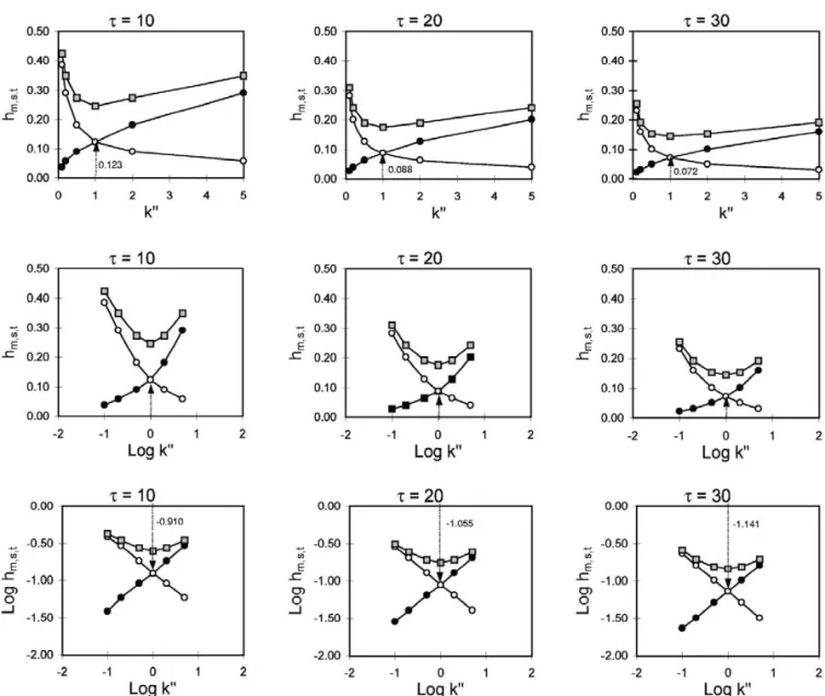
k0 5 1 and n 510, the peak summits were found at Since the peak area (A ) must be conservative,n

positions of P(1,1), P(2,2.5), P(3,4.5),

A ~hW (h the peak height), the widest peak widthn n

P(10,18.5) . . . etc., a 1.5t unit ahead of the migra-occurs at k0 5 1 which refers to the lowest peak

tion route. A general form is given: height h for the total mass. The relationships

be-tween h , h , and h (peak heights for the stationary,s m t _{t 5 t 2 0.5k0 (30)}

r rm

mobile phases and total sum, respectively) and k0

values are shown in Fig. 7. The h (k0) and h (k0)s m where the 0.5k0 term is named the ‘‘temporal shift’’. curves cross at k0 5 1. If taking a logarithmic scale Thus, the chromatographic peak would appear at the for k0, then the two curves are mirror images to each parcel position of n 5N and t 5‘‘the nearest integer other centering at log k0 5 0. If both axes are of (N 2 0.5) (k0 1 1) 2 0.5k0 unless with a decimal logarithmic, then the two curves appear like an ‘‘X’’ of exactly 0.5 time units’’. For example, when k0 5 shape (between 2 1 , log k0 , 1), with slopes of 0.5 0.5 and n 510, the chromatographic peak will be

for log h and 20.5 for log h .s m found at parcel P(10,14); when k0 5 5 and n 510,

Thus, the peak heights for the stationary and the peak summit will appear at P(10,54.5) instead of mobile mass patterns found on the parcel matrix (at a P(10,57) or P(10,60).

Fig. 7. Top, relationships between the mass peak height (h ) and partition ratio (k0) at t 510, 20 and 30, respectively. Middle and bottom,m logarithmic plots for h vs. log k0 and log h vs. log k0 are also presented. The heights for the stationary phase (m ), mobile phase (m ) ands m total (m ) are marked with solid circle, open circle and cube, respectively. Arrows indicate the height data for ht mat k0 5 1 or log hmat log k0 5 0.

chromatography, as similar conclusions have already length (section number), therefore it should not be been demonstrated by Golshan-Shirazi and Guiochon ignored under the linear conditions unless k0 is [13] for at least three types of chromatographic nearly zero.

models including: the plate or tank-in-series model,

the statistical model, and the solutions of the partial 3 .10. Zone width on t coordinate differential equations for mass transfer kinetics along

a column. In those theories the peaks generated all The chromatographic peak shows the mobile-lean toward the left on the time coordinate, and the phase mass fraction only. Since total peak area on t position of the observed peak summit appears slight- coordinate (A ) must be conservative (A 5 A 5 mt t n o

ly earlier than that expected for the mass center. on the parcel matrix), the chromatographic peak will The temporal shift is independent of column appear flatter than does the mass profile. According

to Eq. (16), the standard deviation of a temporal mass center arrives at the detector at t 511, 19 andrm

peak should expand by a factor of k0 1 1 during the 29, respectively. Accordingly, parcels P(10,11), axial transformation. For example, if k0 5 1, then P(10,19) and P(10,29) are chosen as the mapping

s (t ) 5 2s (t ); k0 5 5, s (t ) 5 6s (t ).t r n rm t r n rm centers. By re-plotting the mass profiles on a normal-ized coordinate, i.e. the (2N 2 n)(k0 1 1) axis, and overlapping it onto the temporal peak diagram on a 3

.11. Chromatographic peak in Gaussian form _{normalized t 2 t coordinate, the temporal}

distor-rm

under linear isotherm _{tion effect can be clearly identified.}

For k0 5 0.2, the mass peak is initially asymmetri-Like the mass patterns, chromatographic peaks _{cal. Although it has a comparative quick expanding} generated by the parcel matrix (Fig. 6) can be _{rate but moves fast through the detector, the} chro-approximated by a convoluted Gaussian function _{matographic response implies only a little temporal} [10]. The convolution of Eq. (27) for a given column _{distortion of the spatial pattern. At k0 5 1, the mass} length n 5 N will lead to the following equation: _{profiles are all spatially symmetrical; and therefore} the tailing is completely temporal. For k0 5 2, the m_{o 2[t 2(N 20.5 )(k 011 )] / 2k 0t}2

]]]

m (t) 5m _Œ2pk0t]]e (31) mass peak is asymmetrical and tilting to the reverse

direction. The temporal effect overwhelms the spa-tially fronting fraction, leading to an apparent nor-This equation is quite similar to that derived by de

mal-type tailing. Levie [18]. Although the 0.5 term is not shown in his

The peak mapping also indicates that the temporal equation, he did mention in text that the addition of

effect is minimal when k0 is small or the residence 0.5 gives a better approximation.

time is short; and it becomes dominant when k0 is large or the residence time is long. However, in the 3

.12. Chromatographic peak height _{latter case, the appearance of the peak on the}

recorder chart will be wide and flat, which might The chromatographic peak height h(t ) may ber _{cause most analysts to think that it has become a}

slightly higher than the mass peak height h (t ), i.e.m rm _{Gaussian shape (actually it is not at all times). This}

the mobile-phase mass value in P(N,t ) may ber _{probably explains why the temporal distortion effect}

slightly higher than that in P(N,t ). The difference,rm _{has always been ignored.}

however, is rather small. The peak height that appears on the temporal coordinate can be estimated

by the following equation: _{3 .14. The effect of sample size}

mo 1

]]] ]]

h (N )t ¯ ]]3_Œ] (32) As it has been described in textbooks [2], the

2pt k0

œ

be increased in an exponential trend, and a delay of where trm5 (N 2 0.5)(k0 1 1).

the peak position occurs. The large-size injection can be interpreted as a summation of many small one-3

.13. Temporal distortion under linear isotherms impulse peaks that overlap together, each having a small time lag. However, the resultant peak shape For a mass peak centering at a parcel position P(N, can hardly be expressed by a single equation.

t ), one can compare the mobile mass peak shapesrm The present parcel matrix model provides a con-from both vertical and horizontal directions, after the venient numerical approach for simulating the peak longitudinal axis has been normalized to cope with shapes for various sample sizes. To double the the temporal scaling. Examples of the overlapped sample volume one only needs to input the same peak mappings are shown in Fig. 8. Three k0 values mass number (m ) into both P(0,0) and P(0,1)o

(0.2, 1, and 2) were used to demonstrate three types parcels. For larger sizes one can input a row of data of mass peaks (normal tailing, symmetrical, and along the parcel set P(0,0), P(0,1), P(0,2) . . . and so reverse tailing). For a column length of N 510, the forth. If the incoming sample is continuous, the mass

Fig. 8. Verification of the temporal distortion effect by overlapping spatial and temporal peaks under linear isotherms. Top, mass profiles plotted on 2N 2 n coordinate for k0 5 0.2, 1 and 2, respectively, centering at n 510. Stationary phase, open triangle; mobile phase, black circle; total mass, open square. Middle, chromatographic peaks on the t 2 trmcoordinate for k0 5 0.2, 1 and 2, centering at t 511, 19 and 29, respectively, marked with open circle. Bottom, normalized mapping plots on (20 2 n)(k0 1 1) and t 2 trmcoordinates. The difference between the two curves contributes to the temporal distortion effect.

can be filled from P(0,0) to infinite P(0,t), the Fig. 9a–c). The mass peak position (n ) will have anp

resultant chromatogram will become the ‘‘break- apparent delay, this is because of the late entrance of through curve’’ as can be seen in the frontal analysis. the mass center (Fig. 9d). The migration speed nm

Examples are given in Fig. 9. In this demonstra- seems to be slower than expected in the starting tion the mass and temporal peaks are plotted for five period, but it will reach the normal speed when t is sample sizes (i 51, 2, 5, 10 and 20, respectively). long enough, or after all sample sections have Three k0 values (0.2, 1 and 2) are used. The mobile- entered the column bed.

phase mass profiles are plotted at t 520, and the On the temporal coordinate, all chromatographic temporal chromatographic peaks are plotted at a peaks are in ‘‘distorted mirror-images’’ to the mass

detecting position of n 520. patterns (see Fig. 9f–h). Accordingly, when the

In general, when k0 is small, the increase of the sample size is increased, the peak appearance time sample size will give rise to a ‘‘plateau-like’’ sample will have an extra delay (Fig. 9i). The peak heights zone; and when k0 is large, the mass profile will are also increased depending on the injection size maintain its peak shape, only it is fatter or wider (see and k0 value (Fig. 9j).

Fig. 9. Effects of changing injection sizes (injection sizes i 51, 2, 5, 10 and 20, respectively) on the peak shape and parameters. Left, on the spatial coordinates; right, on the temporal coordinate. (a–c) Mobile-phase mass patterns for k0 5 0.2, 1 and 2, respectively, at time step

t 520. (d) Shift of the mass peak positions with the increase of the injection sizes, n vs. i. (e) Increase of the mass peak height with thep increase of the injection sizes, hmvs. i. (f–h) Chromatographic peak heights for k0 5 0.2, 1 and 2, respectively, as observed at n 520. (i) Delay of the temporal peak position with the increase of the injection sizes, t vs. i. (j) Increase of the temporal peak height with the increaser of the injection sizes, h vs. i.t

4

. Numerical demonstration under non-linear ising chromatographic peak shapes, its usefulness is

isotherms quite limited. When k0 is large, the retention time will be long, and the peak shape will appear to be 4

.1. Conditions of changing isotherms

very ‘‘flat’’. Also, no fronting peak shape will be Although the linear parcel matrix produces prom- generated at any linear circumstance. Therefore it

cannot be applied to simulate the separation of a jection size and mass value are all 1, and the detector

99

variety of components, or to compose a chromato- is placed at n 55. The initial ko value is 8, but

gram as commonly seen in the laboratory. changes to 0.8 at t 511. The impacts on the

migra-However, it should be noted again that what can tion route, peak width and mass patterns are (as be observed on the recorder is just a distorted image, illustrated in Fig. 11) as follows.

not the real spatial pattern. A ‘‘flat’’ chromatographic 1. The migration route turns downward; the t /n peak (on t coordinate) does not mean that the sample ratio changes from 9 to 1.8.

zone is ‘‘wide’’ in the column (on n coordinate). On 2. The expanding rate of the sample zone becomes the contrary, the bandwidth, although invisible to the larger after t 5 11, judging from the standard detector, may still be narrow even if the time is quite deviation or peak width.

long, only the migration speed is slow. If the 3. The mass within a parcel re-distributes after the isotherm can be changed (k0(t) value drops down), it changing. For example, the mass ratio between is possible to release the mass from the stationary the stationary and mobile phases is 8 before phase and to speed up the migration, thus giving a t 510 and becomes 0.8 after t 511. In other

shaper chromatographic peak. words, a substantial fraction of mass is released

In practice, this can be done by elevating tempera- from the stationary phase and appeared in the ture (for GC), increasing the ionic strength or mobile phase. The migration speed is accelerated

altering the polarity of the mobile solvent (for accordingly.

HPLC) [2,3]. In the present model, these conditions 4. The appearance of the chromatographic peak is can be simulated by the programming of k0(t) values earlier with a much higher peak height compared

on a computer worksheet. to that if the k0(t) value was not changed.

4

.2. Effects of changing k0 to peak parameters 4 .3. Temporal distortion when k0(t) changes The sudden change of the k0(t) value of a com- A further verification of the ‘‘spatial tailing’’ or ponent during its migration in a column will prompt- ‘‘temporal tailing’’ is made on a 20360 matrix (Fig. ly influence the migration route, the zone broadening 12). In this demonstration a compound with an initial

99

and the final peak appearance. An example is ko value of 8 is injected (the mass value is 1) into a demonstrated in Fig. 10. In this example, the in- column having a hypothetic detector placed at n 510.

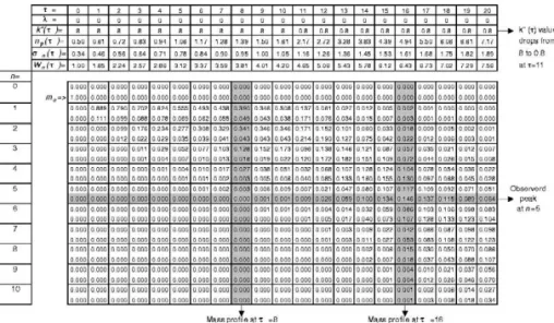
Fig. 10. A 10320 non-linear parcel matrix demonstrates the changing of the migration behaviors of a sample with an initial mass value of

99

1, and an initial k 5 8, which changes from 8 to 0.8 after t 511. The vertical shaded data sets at t 58 and 16 are plotted for the masso profiles, whereas the horizontal shaded data row at n 55 is plotted for the chromatogram (shown in Fig. 11).

Fig. 11. Parameter plots for data generated by the parcel matrix in Fig. 10. (a) The k0(t) value changed from 8 to 0.8 when t 511. (b) The migration route turns downward with a t /n slope of k0(t) 1 1. (c) Expanding of s (t) and W (t) with time steps. (d) Mass profiles for then n

stationary (open circle), mobile (solid circle), and the total (triangle) phases when t 58 (before the k0(t) change). The spatial distribution appears to be fronting. (e) Mass profiles when t 516 after k0 drops to 0.8. The spatial distribution turns out to be quite symmetrical. (f) Response recorded at n 55. The peak appears at t 516 with a significant temporal tailing.

Under the linear isotherm, the migration speed four cases: fronting for k0(t) 5 0.01, nearly

99

(y (t)) is slow, to be Dn (t) /Dt 5 y /(1 1 k ) 5m p o symmetrical for k0(t) 5 0.2, and with a prolonged 0.111. The mass patterns (e.g. when t 520) show a tail for k0(t) 5 1 and 2 (see Fig. 12, top right). The reverse type tailing, with one ninth of the total mass temporal shifts (trm2t ) match exactly the scale ofr

in the mobile phase and the rest (eight ninths) in the 0.5k0(t ), as predicted.rm

stationary phase. If the initial isotherm remains The normalized overlapping of peaks (or residual constant, then the mean residence time for the mass analysis) at the detector position (n 510) when the peak will be: t 5(1020.5)3(811)585.5; therm mass center arrives (t 5 t ) provides the clue torm

appearance of the peak on the temporal coordinate distinguish the spatial and temporal effects. For the will be: t 5 trm2 0.5k0 5 81.5. The retention time above four sets of peaks, the mapping centers were would be too long to observe and the outcome peak chosen at parcel positions of P(10,28), P(10,29),

shape will be very flat. P(10,34) and P(10,42). In Fig. 12, black circles mark

The changing of the isotherm is arranged at t 521, the normalized mobile-phase patterns, whereas open and the k0(t) value is dropped from 8 to 0.01, 0.2, 1 circles mark the observed peaks.

and 2, respectively. The sudden dropping of the k0(t) Case 1 k0(t) value drops from 8 to 0.01 at t 521,

value alters the mass equilibrium between the and the mass peak arrives at the detector at

stationary and mobile phases. The migration routes t 528. The total mass pattern at t 528

bend downward with t /n ratios of 1.01, 1.2, 2, and 3 remains almost the same fronting shape as (see Fig. 12, top left). The mass retention times are that at t 520, but the mass fraction ratio for shortened to t 528, 29, 34.5 and 42, respectively.rm the stationary and mobile phases changes

99

Fig. 12. Demonstration of how the ‘‘isotherm change’’ will affect the peak formation for a compound having an initial ko value of 8. (a)

99

The migration routes on the n 3 t matrix for a component if the k value is changed from 8 to 0.01, 0.2, 1 and 2, respectively at t 521. (b)o The mass profiles at t 520 (before changing). Circle, dot and triangle represent the stationary, mobile and total mass patterns. (c) The resultant chromatographic peaks observed by a detector at n 510. (d) Case 1 (k0 changed to 0.01): the mass profile at t 528 is of a fronting-type; the mobile phase-pattern matches perfectly the temporal image (marked as open cube), leaving no temporal distortion residual. (e) Case 2 (k0 changed to 0.2): the mass profile at t 529 is still fronting; but is slightly less fronting for the temporal image. A very small residual can be seen. (f) Case 3 (k0 changed to 1): the mass profile at t 534 becomes quite symmetrical, but the temporal image carries a tail. The temporal distortion is identified by the residual plot. (g) Case 4 (k0 change to 2): the mass profile at t 542 is nearly Gaussian, and the temporal tailing becomes obvious.

almost identical to the chromatographic (fronting-type) can be considered

exclusive-peak, and the residual analysis shows that ly ‘‘spatial’’.

there is almost no temporal distortion. The Case 2 k0(t) drops to 0.2 and the mass center

fronting and the height is lower than it is in described as: log k0(t)~1 /T. For simplicity, the case 1. The fraction between the stationary relationship is assumed the same for all components. and mobile phases is 1:5. When it is over- The setting of a program for the temperature eleva-lapped on the chromatographic peak, a very tion can be stage-wise, continuous, or first a continu-small residual can be seen. This temporal ous rising then a terminal stage to release those distortion compensates for the spatial front- highly retarding compounds from the column. ing fraction and the resultant outlook is Examples are given in Fig. 13 for four different

99

quite symmetrical. components with initial dynamic partition ratios ko

Case 3 k0(t) drops to 1 and the mass center arrives of 1, 5, 10 and 50, respectively. If these ratios were at t 534.5. Since the parcel addresses are all kept unchanged throughout the operation, then only

99

integers, the data column at t 534 is one peak (k 5 1) could be observed (t 539) for ao rm

plotted. The mass pattern turns out to be column (length520) within the 100 time-step dura-quite symmetrical after the travel period tion.

between t 521 and 34. The mass ratio When the temperature is changed twice (Fig. 13a)

between the stationary and mobile phases is at t 520 and 40, and k0(t) values are dropped to be

99

1:1, and the t /n ratio is 2. The recorder 1 / 2 and 1 / 4 of the initial k , the t /n slopes of theo

gives an obvious normal-type tailing. The migration routes for the four components change temporal distortion is identified by the re- from the initial 2, 6, 11 and 51 to 1, 3, 5.5 and 25.5;

sidual curve analysis. then 0.5, 1.5, 2.75 and 12.25, respectively. The peaks

Case 4 k0(t) drops to 2 and the mass center arrives are sharper in shape, appear earlier, and all carry a at t 542. The mass profiles are nearly normal-type tailing. A little hump is noticed at the Gaussian, but viewed by the recorder to trailing edge of the first peak, marking the changing have a tail. At a t /n ratio of 3, the temporal point at t 540.

distortion becomes even more obvious in In the case of Fig. 13b, since the k0(t) values are proportion. In contrast to case 1, the skew- changed continuously at a decay rate of l50.05 (Eq. ness of the chromatographic peak (pro- (13)), the mass migration routes become concave longed tailing) may be considered exclu- curves. The final k0(t) values when arriving at the

sively ‘‘temporal’’. detector (n 520) are 0.23, 0.45, 0.52 and 0.58,

The shape of the residual curves for the latter two respectively. The corresponding t /n ratios become cases (twisted like an earthworm) is very similar to 1.23, 1.45, 1.52 and 1.58. These slope values are that previously reported for flow injection analysis much lower and lead to higher peak heights and [10]. It has three crossing knots on the horizontal sharper looks. Also, the effect of temporal distortion coordinate, which means that at least three points of is less significant and therefore all peaks look quite the observed peak can be free from the temporal symmetrical.

distortion. However, it should be noted that the In many circumstances a terminal high

tempera-99

expansion forces for the two techniques are different. ture is applied to rush out those high ko value In the present model the expanding is induced only compounds that are still bound to the column. A by the retention behavior in the column, whereas for simulation is given in Fig. 13c, in which the k0(t) FIA it is generated by diffusion. Nonetheless, the value is initially decreased at a decay rate of 0.05

resultant phenomena are similar. and then suddenly dropped to 1 / 100 and maintained

hereafter at t 550. This sudden change will not affect the first peak which has already passed 4

.4. Simulating the temperature programming through the detector, but will accelerate the migra-tion speeds of those that still are retained in the In gas chromatography, the most effective way to column. It is noted that the second peak has a reduce the apparent partition ratio would be the double-summit, one before the drastic temperature increase of temperature. In general, the relationship change and one after. It gives the peak a blunt rising between the k0(t) value and temperature can be edge and a sharp trailing edge, and thus can be

Fig. 13. Temperature programming and how it affects the k0(t) values, migration routes and resultant peak shapes in gas chromatography. Top row, the temperature is programmed to be (a) stage-wise increasing, (b) continuous increasing, and (c) continuous plus a terminal

99

increasing. 2nd row, the change of k0(t) for the four components with initial ko values of 1, 5, 10 and 50, respectively. 3rd row, the mass migration routes for the four components under various isotherms. Dashed line denotes the void position. Bottom row, the chromatogram obtained at n 520. Note that at the changing points some spikes might occur on the peak shoulder.

99

regarded as a temporal fronting-type peak. The third the last peak (initial k 5 50), which ends at a t /no 99

peak, with an initial k 5 10, ends with a k0(t )o rm ratio of 1.08, giving a nearly Gaussian type peak. value of merely 0.016 or a t /n slope of 1.016 when It is interesting to note that all 11 peaks shown in it passes through the detector. The migration speed Fig. 13 are almost Gaussian in the spatial domain (y 5 1 / 1.016y) reaches 98.4% of the flow speed ofm when arriving at the detector, regardless of the the mobile solvent. At this speed the temporal change of the isotherm during the migration. There-distortion is almost diminished, and the observed fore, the peak tailing, fronting, and even the doublet peak shape is almost identical to the spatial pattern, are all spatially ‘‘false’’, as a result of the temporal to be very symmetrical. The same situations apply to distortion effect.

4

.5. Equations for migration routes under non- ₁

2lt

] 99

linear isotherms n (t) 5 0.5 1 t 1p _l ln (k eo 1 1)

1

Although the mass peak position can be calculated _{2]ln (k 1 1)99 (38)}

o

l

by Eq. (18) in a recursion manner on the parcel matrix, it can also be expressed by migration route

The migration routes made by the above equations depending on the conditions of k0(t)

equation agree quite well with that obtained from the programming.

parcel matrix, with very small deviations even when (a) When k0(t) is changed in a stage-wise manner.

t is small (see Fig. 14).

If the changing of k0(t) is made stage-wise with j stages, and changing at t , the position of thej

mass peak on the n coordinate will be: 4 .6. Equations for zone width under non-linear isotherms

1 1

]] ]]

n (t) 5 0.5 1p _{k 1 199} s dt 11 _{k 1 199} (t 2 t )2 1

1 2 _{The recursion calculation of the spatial zone width}

(or standard deviation of a peak) as stated by Eq.

1 . . . (33)

(15) can also be expressed as equations. Accordingly, the general formula for

program-99

ming with j stages each has a kj value of:

j (t 2 tj j 21) ]]] n (t) 5 0.5 1p

O

S

D

(b) When k0(t) is decreased following Eq. (12). If the changing of k0(t) values follows k0(t) 5

99

k (1 2 lt), the migration route will be:o

t 1 ]]]]] n (t) 5 0.5 1p

E

(c) When k0(t) is decreased following Eq. (13). If the changing of k0 value is decreased exponentially (dk0 / dt 5 2 l), the mass peak posi-tion can be predicted approximately by the following

Fig. 14. Examples of using equations to predict (top) the

migra-equation: _{tion route, i.e. Eqs. (22), (34), (36), (38), and (bottom) the zone}

broadening, i.e. Eqs. (24), (40), (42), (45), under various iso-t

99

therms. The initial k values are 10 for all cases. The conditions

1 o

]]]]

n (t) 5 0.5 1p

E

99

k eo 1 1 _{changed from 10 to 1 at t 540 and to 0.2 at t 580, (c) k0(t) is}

0

decreased with a linear decay constant l 5 0.1, (d) k0(t) is decreased with an exponential decay constant l50.1.

]]]]]]]]]

(a) When k0(t) is changed in a stage-wise manner. _{1 1}

2

]]]] ]]]

99

If the initial ko value is changed in j stages s (t) 5 s 1n o 2lt 2_{l(k 1 1)99}

99

l(k e 1 1) o

œ

during the migration (at t , t . . . each has a1 2

99 (45)

k ), the resultant standard deviation will bej

accounted for by:

2lt

When t is large enough or the e term

99

ko

2 2 approaches zero, the band width will no longer

]]] s (t) 5 s 1_{n o 2 1}t

99

(k 1 1)o expand and will converge to the square root of the

99 99

initial variance plus a boundary of [k /(k 1 1)] /l.o o 99

k1

]]] Under this circumstance, all, except the leading

1 2(t 2 t ) 1 . . .2 1 (39)

99

(k 1 1)1 _{peaks (on t coordinate), will be almost identical with}

the same zone width (see Fig. 14d). or,

j ₉₉

kj 21 4 .7. Position of chromatographic peaks

2 2 ]]] s (t) 5 s 1n o

O

s

d

Under non-linear isotherms, the time for the mass peak to migrate to the end of a column of length N (b) When k0(t) is decreased following Eq. (12).

(t ) is quite difficult to calculate directly by a single

If k0(t) is programmed to be decreasing rm

equation (e.g. solving Eqs. (34), (36) or (38) for t

continuously in a linear trend with t, i.e. k0(t) 5 rm

when n (t ) 5 N ), but it can be estimated

graphical-99

k (1 2 lt) and 0 # lt # 1:_o p rm

ly on the matrix. The time for the appearance of the

t

chromatographic peak on t coordinate (t ) is then

99

k (1 2 lt)o r

2 2

]]]]]

s (t) 5 s 1n o

E

99

(k (1 2 lt) 1 1)o

0 _{cases it can be neglected because the final k0(t ) is}

rm

dropped to almost zero when arriving at the detecting then,

point. 1

2 2

]]

F

s (t) 5 s 2n o _lk99 ln (k 2 lk t 1 1)o o _{4 .8. Peak width on t coordinate} o

1

]]]]]

1_{k 2 lk t 1 199 99}

G

o o

deviation of a chromatographic peak for a column

1 1 _{length of N is accounted for by: s (t ) 5 (k0(t ) 1}

t rm rm

]] 99 ]]

1_lk99

F

G

1)s (t ). The peak width W (t ) equals 4s (t ).

o o _{n rm t rm t rm}

Under non-linear isotherms, the extent of peak (c) When k0(t) is decreased following Eq. (13).

distortion is dependent on the zone broadening rate, If k0(t) is programmed to be decreasing

i.e. Ds (t ) /Dt. Therefore when the final k0(t )n m rm

continuously in an exponential trend, i.e. k0(t) 5

drops to near zero, the temporal distortion effect can

2lt

99

k eo , then: _{be very small. However, since k0(t) is still}

decreas-t _{ing before and after arriving at the detector, a small}

2lt

99

k eo

2 2 _{fronting distortion will still occur.}

]]]]

s (t) 5 s 1n o

E

(k eo 1 1)

0

4

.9. Asymmetry transformation on a chromatogram The solution for this integration will be:

In separating a group of compounds, the

chro-1 1

2 2lt 21 21

2 _{] 99 ] 99}

s t 5 s 1ns d o _l(k eo 1 1) 2_l(k 1 1)o _{matogram may comprise of many peaks with various}

shapes. The leading peaks usually appear with (44)

prolonged tails, which are followed by several

have irregular shapes or doublets, and some are decrease exponentially at a decay rate l50.05; (3) nearly symmetrical. In the terminal stage, the last after t 5201, l becomes 0.25.

peaks may have significant fronting tails, which In the linear stage (t 50–50), the leading peaks sometimes exhibit even narrower peak widths and appear with prolonged tails as expected. By compar-higher heights. When these happen, it would be very ing the spatial patterns with chromatographic peaks, puzzling for analysts to explain why and how the it is proven that the spatially-induced tailing fraction peak asymmetry is transformed from ‘‘tailing’’ to is large at the beginning but gradually decreasing

‘‘fronting’’. with time; whereas the temporally-induced tailing

With the aid of the k0(t) programming, it is fraction is small at the beginning, but is gradually possible to create such patterns on the parcel matrix. increasing. At t 551 when the isotherm has been Firstly, the peak shape of each component is gener- changed, the spatial patterns in the column maintain ated individually; then, all peaks are overlapped or a Gaussian shape, but the temporal peak shape combined to compose a complete chromatogram. transforms from tailing to fronting. When the ex-An example is given in Fig. 15. A short column ponential isotherm becomes stable, the peaks that (N 510) is used to separate a group of 18 com- appear during t 5100–200 are all identical in shape,

99

ponents assumed to have initial ko values of 0.2, 0.5, width and height, with a very slight temporal front-1, 1.5, 2, 3, 5, 10, 20, 50, 100, 300, 500, 1000, 3000, ing (so small that they all look like Gaussian curves). 5000, 10 000 and 30 000, respectively. The isotherm Near the second changing point (t 5201), the tempo-has been programmed in three stages: (1) t 50–50, rally-induced fronting effect occurs again, then fades all k0(t) are constant; (2) t 5 51–200, all k0(t) rapidly. In the terminal stage, the peaks appear with slight fronting, which is mainly due to the retardation

99

of those high ko components. The temporal distor-tion effect becomes negligible at the end of the chromatogram as the final k0(t) values are very small.

The fronting caused by the temporal distortion effect may be small under ‘‘stable’’ non-linear isotherms, but can be very obvious near the drastic changing points.

4

.10. Graphical display of the asymmetrical fractions

The peak asymmetry can be expressed by dividing the peak width into two sections at the rising and trailing sides of a peak (Fig. 16). For example, on the longitudinal coordinate, W 5 a 1 b. The massn

pattern is symmetrical when a equals b; and vice versa. Similarly, the width of a chromatographic peak can be expressed as W 5 a9 1 b9. The peakt

shape is symmetrical when a9 5 b9, has a prolonged

Fig. 15. Transformation of peak asymmetry on a chromatogram tail when a9 , b9, and is fronting when a9 . b9. The

as illustrated by a non-linear 103250 parcel matrix programmed _{contribution of the spatial and temporal tailing} to have three-stage isotherms. The exponential decay constant ( l) _{fractions can be identified by comparing the a, b, a9} is 0 during t 50–50, changes to 0.05 during t 551–200, then 0.25

and b9 sections along the migration route at a given

after t 5201. Eighteen components are demonstrated with initial

column length N (marked by a horizontal dashed line

99

ko values of 0.2, 0.5, 1, 1.5, 2, 3, 5, 10, 20, 50, 100, 300, 500,

Fig. 16. Basic peak shapes that were generated by the parcel matrix. The peak widths on n and t coordinates (W and W ) are divided inton t

the leading and trailing sectors, i.e. W 5 a 1 b and W 5 a9 1 b9. The migration routes and zone boundaries are shown on the left, whereasn t

the mass patterns and resultant chromatographic peaks are shown on the right. Conditions for the eight cases (a)–(h), refer to text.

99

In general, eight basic types of peaks can be (a) If the initial ko is very small, the mass peak has identified by the parcel matrix model. Only two a sharp rising edge and a prolonged trailing edge types are related to the spatial reasons, whereas the (a , b). When it arrives at the detector, the rest are all induced by the temporal distortion effect. projected temporal image maintains a similar