Numerical Traveling Wave Solutions of Some
Nonlinear Mixed-type Lattice Differential
Equations
Ching-Lang Huang and Ting-Hui Yang
∗Department of Mathematics, Tamkang University
Tamsui, Taipei County 25137, Taiwan
October 15, 2008
Abstract
We present a finite difference method for computing traveling wave front solutions of a two-dimensional lattice differential equations. In particular, the nonlinear reaction function is bi-stable type and the diffusion term is with function-coupling. Under some suitable con-ditions on the characteristic equation, we prove the existence of the positive wave speed. It can help us to approximate the asymptotically behavior on the boundaries of profile equation. Newton’s method are used to find the solution of nonlinear algebraic equations inducing by the finite difference method. To overcome the difficulty of finding a good initial solution of Newton’s iteration, the continuation method are implemented.
Keywords: Coupling profile equation, Finite difference method, Newton’s iteration, Continuation method.
∗Research supported in part by the National Science Council of Taiwan and the
1
Introduction
The purpose of this paper is to numerically investigate the existence of trav-eling plane wave solutions of the following functional coupling lattice differ-ential equations of the form
dui,j(t)
dt = f (ui,j(t)) + d1g(ui−1,j(t)) + d2g(ui,j−1(t)) −
d3g(ui,j(t)) + d4g(ui+1,j(t)) + d5g(ui,j+1(t)). (1.1)
Here ui,j(t) indicate the state functions located at site (i, j) ∈ Z2; the reaction
function f is bistable type; the coupling function g is sigmoidal type, and the coupling coefficients d1, · · · , d5 are non-negative constants.
The equations (1.1) is so-called lattice differential equations which are infinite system of ordinary differential equations indexed by integer points on R2. If the coefficients d1 = d2 = d4 = d5 = 1 and d3 = 4 and the coupling
function g = id, then equations (1.1) can be viewed as a discretization of the reaction diffusion equation
∂u
∂t(x, t) = 4u(x, t) + f (u(x, t)).
However, such systems can be derived independently from the study of pop-ulation dynamics of biology, dynamics of neural networks, electro-cortical activity of mammalian neocortex, and so on.
Our main concern is to find a traveling wave solution of (1.1) numerically. Let ξ = r1i+r2j +ct be the moving coordinate where r1 = cos(θ), r2 = sin(θ),
0 ≤ θ ≤ π/2. We assume the wave speed c is positive. Under this coordinate xi,j(t) := ϕ(r1i + r2j + ct) := ϕ(ξ), we yield the following nonlinear
mixed-type(delayed and advanced) functional-coupling profile equation c ˙ϕ(ξ) = f (ϕ(ξ)) + d1g(ϕ(ξ − r1)) + d2g(ϕ(ξ − r2)) −
d3g(ϕ(ξ)) + d4g(ϕ(ξ + r1)) + d5g(ϕ(ξ + r2)). (1.2)
The following assumptions will be needed throughout the paper.
(A1) The bistable nonlinearity reaction function f ∈ C1[0, 1] with f (0) =
f (a) = f (1) = 0, a ∈ (0, 0.5), f0(0) < 0, f0(a) > 0, and f0(1) < 0. (A2) The coupling output function g is a monotone increasing C1(R)
func-tion.
(A3) The coupling coefficients are nonnegative real number with d1+ d2−
By the assumption (A3), it follows that there exists homogeneous sta-tionary solutions of (1.2) denoted by
ϕ− := 0, ϕ0 := a, and ϕ+:= 1.
Thus, we are interested in finding a numerical traveling wave solution of (1.2) connecting the two stable equilibria ϕ− and ϕ+ with the asymptotically
boundary conditions
ϕ(−∞) = 0 and ϕ(+∞) = 1. (1.3) The algorithm we discuss here consists of a combination of Newton’s method and parameter continuation method. It is based upon the idea pro-posed in [9, 20]. Our main contribution is to generalize it in two parts. First, the traveling wave solution are computed in a two-dimensional lattice instead of one-dimensional grid. Secondly, functional-coupling effect is consider in discrete diffusion terms.
Recently, the investigation in lattice differential equations analytically[5, 11, 17, 19] or numerically[4, 10] are getting considerable attentions not only from mathematical theory but also from applications in many scientific dis-ciplines. Models involving lattices differential equations can be found in a wealthy of research, including biology [2, 12], chemical reaction theory [8, 13], imaging processing and pattern recognition [6], material science [1, 3], and neural network[6, 15, 16].
The remainder of this paper is organized as follows. In section 2, we will introduce some numerical methods to approximate traveling wave solutions of (1.2). In section 3, some numerical results will be presented for fixed coefficients d1, d2, d3, d4, and d5 while the wave speed c > 0 is solved.
2
Scheme of Solution Approximation
To approximate traveling wave solutions of (1.2) with the asymptotically boundary conditions (1.3), we truncate the real line into a finite interval [−I, I] for I large enough. In section 2.1, we will prove the existence of characteristic roots, λ1 and λ2, of linearized profile equation for ξ < −I and
ξ > I respectively. In section 2.2, traveling wave solutions outside the finite interval [−I, I] can be approximated by exponential functions with λ1 and
λ2. In section 2.3, we take advantage of the finite difference method[14] and
the linear interpolation[18] to approximate the coupling profile equation (1.2) and solve the nonlinear discretized system of (1.2) by Newton’s iteration. In section 2.4, we introduce the continuation method[7] to obtain a sufficiently accurate initial guess for Newton’s iteration. Then we describe the numerical scheme as follows.
2.1
Existence of Characteristic Roots
We first consider the condition ξ < −I. Since ξ → −∞ implies ϕ(ξ) → 0 and f (ϕ(ξ)) → 0, by the linearizaiton of (1.2) near ϕ = 0, we have
c ˙ϕ(ξ) = f0(0)ϕ(ξ) + d1g0(0)ϕ(ξ − r1) + d2g0(0)ϕ(ξ − r2) −
d3g0(0)ϕ(ξ) + d4g0(0)ϕ(ξ + r1) + d5g0(0)ϕ(ξ + r2). (2.1)
Since ϕ(ξ) → 0 as ξ → −∞, we substitute ϕ(ξ) = eλ1ξ, λ1 > 0 into the
equation (2.1) and obtain the following characteristic equation cλ1 = f0(0) + d1g0(0)e−r1λ1 + d2g0(0)e−r2λ1−
d3g0(0) + d4g0(0)er1λ1 + d5g0(0)er2λ1. (2.2)
To prove the existence of λ1, we give the following lemma.
Lemma 2.1. For given wave speed c > 0, if d4g0(0) > 0 or d5g0(0) > 0 then
there exists λ1 > 0 such that the characteristic equation (2.2) has a positive
root.
Proof. We suppose that
L(λ) = f0(0) + d1g0(0)e−r1λ+ d2g0(0)e−r2λ−
d3g0(0) + d4g0(0)er1λ+ d5g0(0)er2λ
is the real-value function then for d4g0(0) > 0 or d5g0(0) > 0, we have
L(0) = f0(0) < 0 and lim
λ→∞L(λ) = ∞ exponentially.
This implies L(λ) and the equation cλ hand over a point λ > 0. Then we can find a λ1 > 0 such that the characteristic equation (2.2) has a positive
root. This completes the proof.
Similarly, if ξ > I with ϕ(ξ) → 1, f (ϕ(ξ)) → 0 as ξ → +∞ then near ϕ = 1, we can obtain the following linearized profile equation
c ˙ϕ(ξ) = −f0(1)(1 − ϕ(ξ)) − d1g0(1)(1 − ϕ(ξ − r1))
−d2g0(1)(1 − ϕ(ξ − r2)) + d3g0(1)(1 − ϕ(ξ))
−d4g0(1)(1 − ϕ(ξ + r1)) − d5g0(1)(1 − ϕ(ξ + r2)). (2.3)
Since ϕ(ξ) → 1 as ξ → +∞, we substitute ϕ(ξ) = 1 − eλ2ξ, λ2 < 0 into the
equation (2.3) and obtain the following characteristic equation cλ2 = f0(1) + d1g0(1)e−r1λ2 + d2g0(1)e−r2λ2−
d3g0(1) + d4g0(1)er1λ2 + d5g0(1)er2λ2. (2.4)
Lemma 2.2. For given wave speed c > 0, if d1g0(1) > 0 or d2g0(1) > 0 then
there exists λ2 < 0 such that the characteristic equation (2.4) has a negative
root. Proof. Let
L(λ) = f0(1) + d1g0(1)e−r1λ+ d2g0(1)e−r2λ−
d3g0(1) + d4g0(1)er1λ+ d5g0(1)er2λ
be the real-value function then for d1g0(1) > 0 or d2g0(1) > 0, we have
L(0) = f0(1) < 0 and lim
λ→−∞L(λ) = ∞ exponentially.
This implies L(λ) and the equation cλ hand over a point λ < 0. Thus, we can find a λ2 < 0 such that the characteristic equation (2.4) has a negative
root.
2.2
Approximate Solutions outside the Finite Interval
We first consider the condition ξ < −I. Since ϕ(ξ) → 0 and f (ϕ(ξ)) → 0 as ξ → −∞, near ϕ = 0, we use the following Taylor expansions
f (ϕ) = a1ϕ + a2ϕ2+ a3ϕ3+ O(ϕ4),
g(ϕ) = b0+ b1ϕ + b2ϕ2+ b3ϕ3+ O(ϕ4)
respectively. Then the coupling profile equation (1.2) becomes c ˙ϕ(ξ) = a1ϕ(ξ) + a2ϕ(ξ)2+ a3ϕ(ξ)3+ d1[b1ϕ(ξ − r1) + b2ϕ(ξ − r1)2+ b3ϕ(ξ − r1)3] + d2[b1ϕ(ξ − r2) + b2ϕ(ξ − r2)2+ b3ϕ(ξ − r2)3] − d3[b1ϕ(ξ) + b2ϕ(ξ)2+ b3ϕ(ξ)3] + d4[b1ϕ(ξ + r1) + b2ϕ(ξ + r1)2+ b3ϕ(ξ + r1)3] + d5[b1ϕ(ξ + r2) + b2ϕ(ξ + r2)2+ b3ϕ(ξ + r2)3]. (2.5)
Since ϕ(−I) → 0 as I → +∞, we consider the formal expansion
ϕ(ξ) = εu1(ξ) + ε2u2(ξ) + ε3u3(ξ) + O(ε4), ε = ϕ(−I) (2.6)
which satisfies the following initial conditions
By the formal expansion (2.6), we can rewrite (2.5) and obtain the following equations c ˙u1(ξ) − Su1(ξ) = 0, (2.7) c ˙u2(ξ) − Su2(ξ) = a2u1(ξ)2+ b2[d1u1(ξ − r1)2 + d2u1(ξ − r2)2− d3u1(ξ)2+ d4u1(ξ + r1)2+ d5u1(ξ + r2)2], (2.8) c ˙u3(ξ) − Su3(ξ) = a3u1(ξ)3+ b3[d1u1(ξ − r1)3+ d2u1(ξ − r2)3− d3u1(ξ)3+ d4u1(ξ + r1)3+ d5u1(ξ + r2)3] + 2{a2u1(ξ)u2(ξ) + b2[d1u1(ξ − r1)u2(ξ − r1) + d2u1(ξ − r2)u2(ξ − r2) − d3u1(ξ)u2(ξ) + (2.9) d4u1(ξ + r1)u2(ξ + r1) + d5u1(ξ + r2)u2(ξ + r2)]},
where the operator S is defined by
Su(ξ) = a1u(ξ) + d1b1u(ξ − r1) + d2b1u(ξ − r2) −
d3b1u(ξ) + d4b1u(ξ + r1) + d5b1u(ξ + r2).
Since the equation (2.7) is linear and homogeneous, a solution to (2.7) which satisfies u1(−I) = 1 is
u1(ξ) = eλ1(ξ+I), λ1 > 0.
A particular solution of the nonhomogeneous equation (2.8) is up2(ξ) = k1e2λ1(ξ+I)
where k1 = a2+ b2Γ1 2cλ1− a1 − b1Γ1 with Γ1 = d1e−2r1λ1 + d2e−2r2λ1 − d3+ d4e2r1λ1 + d5e2r2λ1.
Since a solution of (2.8) satisfies u2(−I) = 0, we have
u2(ξ) = k1(e2λ1(ξ+I)− eλ1(ξ+I)).
We suppose that up3(ξ) = k2e2λ1(ξ+I)+ k3e3λ1(ξ+I) is a particular solution of
the nonhomogeneous equation (2.9) where k2 =
−2k1(a2+ b2Γ1)
2cλ1− a1− b1Γ1
and k3 = (2a2k1+ a3) + (2b2k1+ b3)Γ2 3cλ1− a1 − b1Γ2 with Γ2 = d1e−3r1λ1 + d2e−3r2λ1 − d3+ d4e3r1λ1 + d5e3r2λ1.
Since a solution of (2.9) satisfies u3(−I) = 0, we obtain
u3(ξ) = k2e2λ1(ξ+I)+ k3e3λ1(ξ+I)− (k2+ k3)eλ1(ξ+I).
Thus, if ξ < −I then with ε = ϕ(−I),
ϕ(ξ) ≈ εeλ1(ξ+I)+ ε2k1(e2λ1(ξ+I)− eλ1(ξ+I)) +
ε3[k2e2λ1(ξ+I)+ k3e3λ1(ξ+I)− (k2+ k3)eλ1(ξ+I)]. (2.10)
Similarly, if ξ > I with ϕ(ξ) → 1, f (ϕ(ξ)) → 0 as ξ → +∞ then near ϕ = 1, we consider the following Taylor expansions
f (ϕ) = A1(1 − ϕ) + A2(1 − ϕ)2+ A3(1 − ϕ)3+ O((1 − ϕ)4),
g(ϕ) = B0+ B1(1 − ϕ) + B2(1 − ϕ)2+ B3(1 − ϕ)3+ O((1 − ϕ)4)
respectively. Then the coupling profile equation (1.2) becomes c ˙ϕ(ξ) = A1(1 − ϕ(ξ)) + A2(1 − ϕ(ξ))2+ A3(1 − ϕ(ξ))3+ d1[B1(1 − ϕ(ξ − r1)) + B2(1 − ϕ(ξ − r1))2+ B3(1 − ϕ(ξ − r1))3] + d2[B1(1 − ϕ(ξ − r2)) + B2(1 − ϕ(ξ − r2))2+ B3(1 − ϕ(ξ − r2))3] − d3[B1(1 − ϕ(ξ)) + B2(1 − ϕ(ξ))2+ B3(1 − ϕ(ξ))3] + (2.11) d4[B1(1 − ϕ(ξ + r1)) + B2(1 − ϕ(ξ + r1))2+ B3(1 − ϕ(ξ + r1))3] + d5[B1(1 − ϕ(ξ + r2)) + B2(1 − ϕ(ξ + r2))2+ B3(1 − ϕ(ξ + r2))3].
Since ϕ(I) → 1 as I → +∞, we consider the formal expansion
ϕ(ξ) = 1 − δv1(ξ) − δ2v2(ξ) − δ3v3(ξ) + O(δ4), δ = 1 − ϕ(I) (2.12)
which satisfy the following initial conditions
v1(I) = 1 and v2(I) = v3(I) = 0.
By the formal expansion (2.12), we can rewrite (2.11) and obtain the following equations
c ˙v2(ξ) − T v2(ξ) = −A2v1(ξ)2− B2[d1v1(ξ − r1)2+ d2v1(ξ − r2)2− d3v1(ξ)2 + d4v1(ξ + r1)2+ d5v1(ξ + r2)2], (2.14) c ˙v3(ξ) − T v3(ξ) = −A3v1(ξ)3− B3[d1v1(ξ − r1)3+ d2v1(ξ − r2)3− d3v1(ξ)3+ d4v1(ξ + r1)3+ d5v1(ξ + r2)3] − 2{A2v1(ξ)v2(ξ) + B2[d1v1(ξ − r1)v2(ξ − r1) + d2v1(ξ − r2)v2(ξ − r2) − d3v1(ξ)v2(ξ) + (2.15) d4v1(ξ + r1)v2(ξ + r1) + d5v1(ξ + r2)v2(ξ + r2)]},
where the operator T is defined by
T v(ξ) = −A1v(ξ) − d1B1v(ξ − r1) − d2B1v(ξ − r2) +
d3B1v(ξ) − d4B1v(ξ + r1) − d5B1v(ξ + r2).
Since the equation (2.13) is linear and homogeneous, a solution to (2.13) which satisfies v1(I) = 1 is
v1(ξ) = eλ2(ξ−I), λ2 < 0.
A particular solution of the nonhomogeneous (2.14) is v2p(ξ) = m1e2λ2(ξ−I)
where m1 = −A2− B2η1 2cλ2+ A1+ B1η1 with η1 = d1e−2r1λ2+ d2e−2r2λ2 − d3+ d4e2r1λ2 + d5e2r2λ2.
Since a solution of (2.14) satisfies v2(I) = 0, we have
v2(ξ) = m1(e2λ2(ξ−I)− eλ2(ξ−I)).
We suppose that vp3(ξ) = m2e2λ2(ξ−I)+ m3e3λ2(ξ−I) is a particular solution of
the nonhomogeneous equation (2.15) where m2 = 2m1(A2+ B2η1) 2cλ2+ A1+ B1η1 = −2m21, and m3 = −(2A2m1+ A3) − (2B2m1+ B3)η2 3cλ2+ A1+ B1η2 with
η2 = d1e−3r1λ2+ d2e−3r2λ2 − d3+ d4e3r1λ2 + d5e3r2λ2.
Since a solution of (2.15) satisfies v3(I) = 0, we obtain
v3(ξ) = m2e2λ2(ξ−I)+ m3e3λ2(ξ−I)− (m2+ m3)eλ2(ξ−I).
Thus, if ξ > I then with δ = 1 − ϕ(I), ϕ(ξ) ≈ 1 − δeλ2(ξ−I)− δ2m
1(e2λ2(ξ−I)− eλ2(ξ−I)) −
δ3[m2e2λ2(ξ−I)+ m3e3λ2(ξ−I)− (m2+ m3)eλ2(ξ−I)]. (2.16)
2.3
Finite Difference Method
To approximate traveling wave solutions inside [−I, I], we first discretize the finite interval [−I, I] and use a fixed, uniform step size h = 2I/N . Then we define the following notations
ξj = −I + jh, ϕ(ξj) := ϕj for j = 0, 1, ..., N. (2.17)
By the finite difference method for five-points formula, we can approximate the first derivative term ˙ϕ(ξ) of (1.2) is then
˙
ϕ(ξ) = 1
12h[ϕ(ξ − 2h) − 8ϕ(ξ − h) + 8ϕ(ξ + h) − ϕ(ξ + 2h)] + O(h
4).
Thus, by the notations of (2.17), we have ˙
ϕ(ξ) ≈ 1
12h(ϕj−2− 8ϕj−1+ 8ϕj+1− ϕj+2). (2.18) As j = 0 and j = 1, terms ϕ−2 and ϕ−1 appear on the right-hand side of
(2.18). Then we use the formula (2.10) for ξ = −I − 2h and ξ = −I − h to approximate these terms respectively. Similarly, if j = N − 1 and j = N then ϕN +1and ϕN +2can be approximated by the formula (2.16) for ξ = I + h and
ξ = I + 2h respectively.
For the delayed and the advanced terms in (1.2), we take advantage of the cubic interpolation to approximate them. Let M1 = [r1h] and M2 = [r2h]
with s1 = r1 − M1h ≥ 0, s2 = r2− M2h ≥ 0 where ”[x]” means the integer
part of x. Then ξ − r1 lies between ξ − M1h − h and ξ − M1h. Similarly,
ξ − r2 lies between ξ − M2h − h and ξ − M2h. By the cubic formula
ϕ(ξ − r1) = x4ϕ(ξ − M1h − 2h) + x3ϕ(ξ − M1h − h) +
where the xi’s are the following constants x1 = −(2h − s1)(h − s1)s1 6h3 x2 = (2h − s1)(h − s1)(h + s1) 2h3 x3 = (2h − s1)(h + s1)s1 2h3 x4 = −(h + s1)(h − s1)s1 6h3 and ϕ(ξ − r2) = y4ϕ(ξ − M2h − 2h) + y3ϕ(ξ − M2h − h) + y2ϕ(ξ − M2h) + y1ϕ(ξ − M2h + h) + O(h4)
where the yi’s are the following constants
y1 = −(2h − s2)(h − s2)s2 6h3 y2 = (2h − s2)(h − s2)(h + s2) 2h3 y3 = (2h − s2)(h + s2)s2 2h3 y4 = −(h + s2)(h − s2)s2 6h3
Thus, the delayed terms can be approximated by
ϕ(ξ − r1) ≈ x4ϕj−M1−2+ x3ϕj−M1−1+ x2ϕj−M1 + x1ϕj−M1+1 (2.19)
and
ϕ(ξ − r2) ≈ y4ϕj−M2−2+ y3ϕj−M2−1+ y2ϕj−M2 + y1ϕj−M2+1. (2.20)
Similarly, we can approximate the advanced terms by
ϕ(ξ + r1) ≈ x1ϕj+M1−1+ x2ϕj+M1 + x3ϕj+M1+1+ x4ϕj+M1+2 (2.21)
and
By using (2.18) to (2.22), we can discretize the coupling profile equation (1.2) and obtain the following nonlinear discretized system
c 12h(ϕj−2− 8ϕj−1+ 8ϕj+1− ϕj+2) − f (ϕj) + d3g(ϕj) −d1g(x4ϕj−M1−2+ x3ϕj−M1−1+ x2ϕj−M1 + x1ϕj−M1+1) −d2g(y4ϕj−M2−2+ y3ϕj−M2−1+ y2ϕj−M2 + y1ϕj−M2+1) −d4g(x1ϕj+M1−1+ x2ϕj+M1 + x3ϕj+M1+1+ x4ϕj+M1+2) −d5g(y1ϕj+M2−1+ y2ϕj+M2 + y3ϕj+M2+1+ y4ϕj+M2+2) = 0 for j = 0, 1, ..., N. (2.23) In the system (2.23), the ϕj’s for j < 0 are functions of ϕ0 then we can
use (2.10) with ε = ϕ0 to approximate them. As the ϕj’s for j > N relate
to ϕN, ϕj are evaluated by (2.16) with δ = 1 − ϕN. However, there are
(N + 1) equations and (N + 2) unknowns c, ϕ0, ϕ1, ..., ϕN in the discretized
system (2.23). This causes the system (2.23) to have no the unique solution. Hence, we add in ϕN/2− 0.5 = 0 as the (N + 2)th equation of (2.23) since
the condition ϕ(0) = 0.5 is autonomous, time translates of solutions are also solutions.
There are many possible ways of solving the system (2.23). Here we design a nested iteration scheme in which c is fixed during the inner loop. The outer loop is the solution of an equation h(c) = 0 by the secant method where the function h(c) is defined as follows.
Definition 2.3. For fixed wave speed c > 0, we solve the nonlinear system of (N + 1) equations F = (2.23) for j = 0, 1, ..., (N2 − 1) ϕN/2− 0.5 (2.23) for j = (N 2 + 1), ..., N . (2.24)
Then we define h(c) = left-hand side of (2.23) for j = N/2.
To solve the nonlinear system (2.24), we use Newton’s iteration during the inner loop. Given the initial guess Φ(0), a sequence of iteration Φ(k) =
{(ϕ(k)0 , ϕ(k)1 , ..., ϕ(k)n ), k = 0, 1, ...} is generated. The sequence Φ(k) converges
to the solution if Φ(0) is sufficiently close to the solution and the Jacobian matrix J which is approximated by centered-difference method is nonsingular at the solution. However, the weakness in Newton’s iteration arises from the need to compute and invert the Jacobian matrix J at each step. Thus we perform a two-step operation to avoid explicit computation of J−1. First, we solve the linear system J (Φ(k−1))y = −F (Φ(k−1)) for a vector y at each stage
of iteration. Then the new approximation Φ(k) is obtained by adding y to Φ(k−1).
2.4
Continuation Method
How to get a good initial guess for the Newton’s iteration? At first, we can solve the nonlinear function fewith the exact solution, ϕ(ξ) = (1+tanh(ξ))/2
is given. Let k := tanh(ξ) := 2ϕ(ξ) − 1 then ˙ϕ(ξ) = (1 − tanh2(ξ))/2 = (1 − k2)/2 and the coupling profile equation (1.2) becomes
c(1 − k 2 2 ) = fe(ϕ) + d1g( (1 − P1)ϕ 1 − P1k ) + d2g( (1 − P2)ϕ 1 − P2k ) − d3g(ϕ) + d4g( (1 + P1)ϕ 1 + P1k ) + d5g( (1 + P2)ϕ 1 + P2k ). Hence, we obtain the exactly form of f is then
fe(ϕ) = c( 1 − k2 2 ) − d1g( (1 − P1)ϕ 1 − P1k ) − d2g( (1 − P2)ϕ 1 − P2k ) + d3g(ϕ) − d4g( (1 + P1)ϕ 1 + P1k ) − d5g( (1 + P2)ϕ 1 + P2k ) (2.25) where P1 = tanh(r1) and P2 = tanh(r2). It’s difficult for Newton’s iteration
to ensure the initial guess which is close to the solution. Thus, we take advantage of the continuation method to approach the solution we want. The way of the continuation method is as follows.
At first, we consider the nonlinear reaction function f of (1.2) which represents our ”target function” and add the coupling profile equation (1.2) in the following one-parameter family of equations
c ˙ϕ(ξ) = fα(ϕ(ξ)) + d1g(ϕ(ξ − r1)) + d2g(ϕ(ξ − r2)) −
d3g(ϕ(ξ)) + d4g(ϕ(ξ + r1)) + d5g(ϕ(ξ + r2)), (2.26)
with asymptotically boundary conditions, ϕ(−∞) = 0 and ϕ(+∞) = 1 where fα(ϕ) = αf (ϕ) + (1 − α)fe(ϕ), 0 ≤ α ≤ 1,
and fe(ϕ) is given by (2.25).
Then we compute approximate solutions from α = 0 to α = 1. As α = 0, we have fα(ϕ) = fe(ϕ) then the exactly solution ϕ(ξ) = (1 + tanh(ξ))/2 is
used as the initial guess to solve the correspond discrete system (2.23). Once a equation for α = 0 is solved, we increase α adaptively and use the solution to previous equation as the initial approximation to obtain the solution to the next equation. As α = 1, we just have solved the equation for fα(ϕ) = f (ϕ)
3
Numerical Results
In this section, we will present the numerical results with two different function-coupling in diffusion term, the identity and the hypertangent func-tion, in Section 3.1 and 3.2. The algorithm are implemented in MATLAB 1c
program with the fixed uniformly step size h = 0.05 and the error accuracy of Newton’s iteration ε = 10−4.
3.1
The coupling function g is Identity
In this section, we consider the monotone increasing coupling output function g(ϕ) = ϕ. Given the classical coupling coefficients d1 = 1.0, d2 = 1.0,
d3 = 4.0, d4 = 1.0, and d5 = 1.0. It is interested for us to investigate the
convergence of numerical traveling wave solutions as θ less vary from θ = 0 to θ = π/2. Thus, the conditions we test are as follows.
At first, we frame a = 0.05 and choose some particular angles to observe the convergence of numerical solutions for continuation method. Then we obtain the following results.
−3 −2 −1 0 1 2 3 0 0.1 0.2 0.3 0.4 0.5 0.6 0.7 0.8 0.9 1 a = 0.05 b = 15.0 d1 = 1.0 d2 = 1.0 d3 = 4.0 d4 = 1.0 d5 = 1.0 a = 0.05 b = 15.0 d1 = 1.0 d2 = 1.0 d3 = 4.0 d4 = 1.0 d5 = 1.0 a = 0.05 b = 15.0 d1 = 1.0 d2 = 1.0 d3 = 4.0 d4 = 1.0 d5 = 1.0 a = 0.05 b = 15.0 d1 = 1.0 d2 = 1.0 d3 = 4.0 d4 = 1.0 d5 = 1.0 a = 0.05 b = 15.0 d1 = 1.0 d2 = 1.0 d3 = 4.0 d4 = 1.0 d5 = 1.0 a = 0.05 b = 15.0 d1 = 1.0 d2 = 1.0 d3 = 4.0 d4 = 1.0 d5 = 1.0 a = 0.05 b = 15.0 d1 = 1.0 d2 = 1.0 d3 = 4.0 d4 = 1.0 d5 = 1.0 a = 0.05 b = 15.0 d1 = 1.0 d2 = 1.0 d3 = 4.0 d4 = 1.0 d5 = 1.0 a = 0.05 b = 15.0 d1 = 1.0 d2 = 1.0 d3 = 4.0 d4 = 1.0 d5 = 1.0 a = 0.05 b = 15.0 d1 = 1.0 d2 = 1.0 d3 = 4.0 d4 = 1.0 d5 = 1.0 Figure 1. θ = 0
−3 −2 −1 0 1 2 3 0 0.1 0.2 0.3 0.4 0.5 0.6 0.7 0.8 0.9 1 a = 0.05 b = 15.0 d1 = 1.0 d2 = 1.0 d3 = 4.0 d4 = 1.0 d5 = 1.0 a = 0.05 b = 15.0 d1 = 1.0 d2 = 1.0 d3 = 4.0 d4 = 1.0 d5 = 1.0 a = 0.05 b = 15.0 d1 = 1.0 d2 = 1.0 d3 = 4.0 d4 = 1.0 d5 = 1.0 a = 0.05 b = 15.0 d1 = 1.0 d2 = 1.0 d3 = 4.0 d4 = 1.0 d5 = 1.0 a = 0.05 b = 15.0 d1 = 1.0 d2 = 1.0 d3 = 4.0 d4 = 1.0 d5 = 1.0 a = 0.05 b = 15.0 d1 = 1.0 d2 = 1.0 d3 = 4.0 d4 = 1.0 d5 = 1.0 a = 0.05 b = 15.0 d1 = 1.0 d2 = 1.0 d3 = 4.0 d4 = 1.0 d5 = 1.0 a = 0.05 b = 15.0 d1 = 1.0 d2 = 1.0 d3 = 4.0 d4 = 1.0 d5 = 1.0 a = 0.05 b = 15.0 d1 = 1.0 d2 = 1.0 d3 = 4.0 d4 = 1.0 d5 = 1.0 Figure 2. θ = π/4 −3 −2 −1 0 1 2 3 0 0.1 0.2 0.3 0.4 0.5 0.6 0.7 0.8 0.9 1 a = 0.05 b = 15.0 d1 = 1.0 d2 = 1.0 d3 = 4.0 d4 = 1.0 d5 = 1.0 a = 0.05 b = 15.0 d1 = 1.0 d2 = 1.0 d3 = 4.0 d4 = 1.0 d5 = 1.0 a = 0.05 b = 15.0 d1 = 1.0 d2 = 1.0 d3 = 4.0 d4 = 1.0 d5 = 1.0 a = 0.05 b = 15.0 d1 = 1.0 d2 = 1.0 d3 = 4.0 d4 = 1.0 d5 = 1.0 a = 0.05 b = 15.0 d1 = 1.0 d2 = 1.0 d3 = 4.0 d4 = 1.0 d5 = 1.0 a = 0.05 b = 15.0 d1 = 1.0 d2 = 1.0 d3 = 4.0 d4 = 1.0 d5 = 1.0 a = 0.05 b = 15.0 d1 = 1.0 d2 = 1.0 d3 = 4.0 d4 = 1.0 d5 = 1.0 a = 0.05 b = 15.0 d1 = 1.0 d2 = 1.0 d3 = 4.0 d4 = 1.0 d5 = 1.0 a = 0.05 b = 15.0 d1 = 1.0 d2 = 1.0 d3 = 4.0 d4 = 1.0 d5 = 1.0 a = 0.05 b = 15.0 d1 = 1.0 d2 = 1.0 d3 = 4.0 d4 = 1.0 d5 = 1.0 Figure 3. θ = π/2
Table 1. θ = 0, π/4, π/2 θ Converges ? α c
0 Yes 1.00 2.289
π/4 Yes 1.00 2.368
π/2 Yes 1.00 2.289
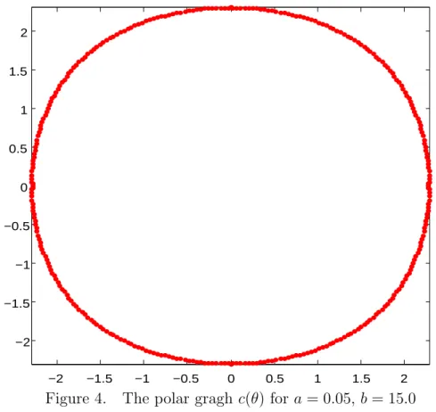
As θ less increase from θ = 0 to θ = π/2, we can obtain the following c − θ polar coordinate figure.
−2 −1.5 −1 −0.5 0 0.5 1 1.5 2 −2 −1.5 −1 −0.5 0 0.5 1 1.5 2
Figure 4. The polar gragh c(θ) for a = 0.05, b = 15.0
Consider a = 0.1 and choose the particular angles, θ = 0, θ = π/4, and θ = π/2 to observe the convergence of numerical solutions for continuation method. Then we have the following results.
−30 −2 −1 0 1 2 3 0.1 0.2 0.3 0.4 0.5 0.6 0.7 0.8 0.9 1 a = 0.1 b = 15.0 d1 = 1.0 d2 = 1.0 d3 = 4.0 d4 = 1.0 d5 = 1.0 a = 0.1 b = 15.0 d1 = 1.0 d2 = 1.0 d3 = 4.0 d4 = 1.0 d5 = 1.0 a = 0.1 b = 15.0 d1 = 1.0 d2 = 1.0 d3 = 4.0 d4 = 1.0 d5 = 1.0 a = 0.1 b = 15.0 d1 = 1.0 d2 = 1.0 d3 = 4.0 d4 = 1.0 d5 = 1.0 a = 0.1 b = 15.0 d1 = 1.0 d2 = 1.0 d3 = 4.0 d4 = 1.0 d5 = 1.0 a = 0.1 b = 15.0 d1 = 1.0 d2 = 1.0 d3 = 4.0 d4 = 1.0 d5 = 1.0 a = 0.1 b = 15.0 d1 = 1.0 d2 = 1.0 d3 = 4.0 d4 = 1.0 d5 = 1.0 a = 0.1 b = 15.0 d1 = 1.0 d2 = 1.0 d3 = 4.0 d4 = 1.0 d5 = 1.0 a = 0.1 b = 15.0 d1 = 1.0 d2 = 1.0 d3 = 4.0 d4 = 1.0 d5 = 1.0 a = 0.1 b = 15.0 d1 = 1.0 d2 = 1.0 d3 = 4.0 d4 = 1.0 d5 = 1.0 Figure 5. θ = 0 −30 −2 −1 0 1 2 3 0.1 0.2 0.3 0.4 0.5 0.6 0.7 0.8 0.9 1 a = 0.1 b = 15.0 d1 = 1.0 d2 = 1.0 d3 = 4.0 d4 = 1.0 d5 = 1.0 a = 0.1 b = 15.0 d1 = 1.0 d2 = 1.0 d3 = 4.0 d4 = 1.0 d5 = 1.0 a = 0.1 b = 15.0 d1 = 1.0 d2 = 1.0 d3 = 4.0 d4 = 1.0 d5 = 1.0 a = 0.1 b = 15.0 d1 = 1.0 d2 = 1.0 d3 = 4.0 d4 = 1.0 d5 = 1.0 a = 0.1 b = 15.0 d1 = 1.0 d2 = 1.0 d3 = 4.0 d4 = 1.0 d5 = 1.0 a = 0.1 b = 15.0 d1 = 1.0 d2 = 1.0 d3 = 4.0 d4 = 1.0 d5 = 1.0 a = 0.1 b = 15.0 d1 = 1.0 d2 = 1.0 d3 = 4.0 d4 = 1.0 d5 = 1.0 a = 0.1 b = 15.0 d1 = 1.0 d2 = 1.0 d3 = 4.0 d4 = 1.0 d5 = 1.0 a = 0.1 b = 15.0 d1 = 1.0 d2 = 1.0 d3 = 4.0 d4 = 1.0 d5 = 1.0 Figure 6. θ = π/4
−30 −2 −1 0 1 2 3 0.1 0.2 0.3 0.4 0.5 0.6 0.7 0.8 0.9 1 a = 0.1 b = 15.0 d1 = 1.0 d2 = 1.0 d3 = 4.0 d4 = 1.0 d5 = 1.0 a = 0.1 b = 15.0 d1 = 1.0 d2 = 1.0 d3 = 4.0 d4 = 1.0 d5 = 1.0 a = 0.1 b = 15.0 d1 = 1.0 d2 = 1.0 d3 = 4.0 d4 = 1.0 d5 = 1.0 a = 0.1 b = 15.0 d1 = 1.0 d2 = 1.0 d3 = 4.0 d4 = 1.0 d5 = 1.0 a = 0.1 b = 15.0 d1 = 1.0 d2 = 1.0 d3 = 4.0 d4 = 1.0 d5 = 1.0 a = 0.1 b = 15.0 d1 = 1.0 d2 = 1.0 d3 = 4.0 d4 = 1.0 d5 = 1.0 a = 0.1 b = 15.0 d1 = 1.0 d2 = 1.0 d3 = 4.0 d4 = 1.0 d5 = 1.0 a = 0.1 b = 15.0 d1 = 1.0 d2 = 1.0 d3 = 4.0 d4 = 1.0 d5 = 1.0 a = 0.1 b = 15.0 d1 = 1.0 d2 = 1.0 d3 = 4.0 d4 = 1.0 d5 = 1.0 a = 0.1 b = 15.0 d1 = 1.0 d2 = 1.0 d3 = 4.0 d4 = 1.0 d5 = 1.0 Figure 7. θ = π/2 Table 2. θ = 0, π/4, π/2 θ Converges ? α c 0 Yes 1.00 1.982 π/4 Yes 1.00 2.071 π/2 Yes 1.00 1.982
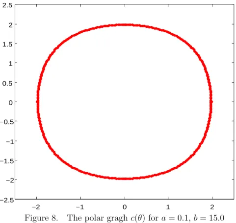
As θ less increase from θ = 0 to θ = π/2, we can obtain the following c − θ polar coordinate figure.
−2 −1 0 1 2 −2.5 −2 −1.5 −1 −0.5 0 0.5 1 1.5 2 2.5
Figure 8. The polar gragh c(θ) for a = 0.1, b = 15.0
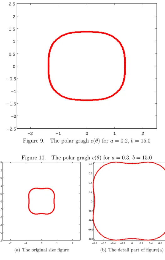
Similarly to previous analysis, we arrive at the following Figure 9 and Figure 10.
−2 −1 0 1 2 −2.5 −2 −1.5 −1 −0.5 0 0.5 1 1.5 2 2.5
Figure 9. The polar gragh c(θ) for a = 0.2, b = 15.0
Figure 10. The polar gragh c(θ) for a = 0.3, b = 15.0
−2 −1 0 1 2 −2.5 −2 −1.5 −1 −0.5 0 0.5 1 1.5 2 2.5
(a) The original size figure
−0.8 −0.6 −0.4 −0.2 0 0.2 0.4 0.6 0.8 −0.8 −0.6 −0.4 −0.2 0 0.2 0.4 0.6 0.8
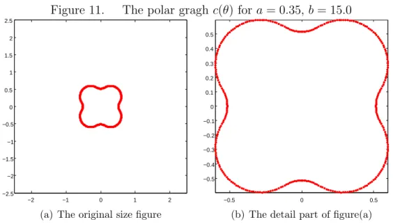
Figure 11. The polar gragh c(θ) for a = 0.35, b = 15.0 −2 −1 0 1 2 −2.5 −2 −1.5 −1 −0.5 0 0.5 1 1.5 2 2.5
(a) The original size figure
−0.5 0 0.5 −0.5 −0.4 −0.3 −0.2 −0.1 0 0.1 0.2 0.3 0.4 0.5
(b) The detail part of figure(a)
3.2
The coupling function g is a Hyper-Tangent Map
Here we frame the coupling output function g(ϕ) = (1 + tanh(ϕ))/2. Given the coupling coefficients d1 = 1.0, d2 = 1.0, d3 = 4.4, d4 = 1.2, and d5 = 1.2.
To investigate the convergence of numerical traveling wave solutions as θ less vary from θ = 0 to θ = π/2, we test the following conditions.
At first, we frame a = 0.05 and choose some particular angles to observe the convergence of numerical solutions for continuation method. Then the results we obtain are as follows.
−30 −2 −1 0 1 2 3 0.1 0.2 0.3 0.4 0.5 0.6 0.7 0.8 0.9 1 a = 0.05 b = 15.0 d1 = 1.0 d2 = 1.0 d3 = 4.4 d4 = 1.2 d5 = 1.2 a = 0.05 b = 15.0 d1 = 1.0 d2 = 1.0 d3 = 4.4 d4 = 1.2 d5 = 1.2 a = 0.05 b = 15.0 d1 = 1.0 d2 = 1.0 d3 = 4.4 d4 = 1.2 d5 = 1.2 a = 0.05 b = 15.0 d1 = 1.0 d2 = 1.0 d3 = 4.4 d4 = 1.2 d5 = 1.2 a = 0.05 b = 15.0 d1 = 1.0 d2 = 1.0 d3 = 4.4 d4 = 1.2 d5 = 1.2 a = 0.05 b = 15.0 d1 = 1.0 d2 = 1.0 d3 = 4.4 d4 = 1.2 d5 = 1.2 a = 0.05 b = 15.0 d1 = 1.0 d2 = 1.0 d3 = 4.4 d4 = 1.2 d5 = 1.2 a = 0.05 b = 15.0 d1 = 1.0 d2 = 1.0 d3 = 4.4 d4 = 1.2 d5 = 1.2 a = 0.05 b = 15.0 d1 = 1.0 d2 = 1.0 d3 = 4.4 d4 = 1.2 d5 = 1.2 Figure 12. θ = 0 −30 −2 −1 0 1 2 3 0.1 0.2 0.3 0.4 0.5 0.6 0.7 0.8 0.9 1 a = 0.05 b = 15.0 d1 = 1.0 d2 = 1.0 d3 = 4.4 d4 = 1.2 d5 = 1.2 a = 0.05 b = 15.0 d1 = 1.0 d2 = 1.0 d3 = 4.4 d4 = 1.2 d5 = 1.2 a = 0.05 b = 15.0 d1 = 1.0 d2 = 1.0 d3 = 4.4 d4 = 1.2 d5 = 1.2 a = 0.05 b = 15.0 d1 = 1.0 d2 = 1.0 d3 = 4.4 d4 = 1.2 d5 = 1.2 a = 0.05 b = 15.0 d1 = 1.0 d2 = 1.0 d3 = 4.4 d4 = 1.2 d5 = 1.2 a = 0.05 b = 15.0 d1 = 1.0 d2 = 1.0 d3 = 4.4 d4 = 1.2 d5 = 1.2 a = 0.05 b = 15.0 d1 = 1.0 d2 = 1.0 d3 = 4.4 d4 = 1.2 d5 = 1.2 a = 0.05 b = 15.0 d1 = 1.0 d2 = 1.0 d3 = 4.4 d4 = 1.2 d5 = 1.2 a = 0.05 b = 15.0 d1 = 1.0 d2 = 1.0 d3 = 4.4 d4 = 1.2 d5 = 1.2 Figure 13. θ = π/4
−30 −2 −1 0 1 2 3 0.1 0.2 0.3 0.4 0.5 0.6 0.7 0.8 0.9 1 a = 0.05 b = 15.0 d1 = 1.0 d2 = 1.0 d3 = 4.4 d4 = 1.2 d5 = 1.2 a = 0.05 b = 15.0 d1 = 1.0 d2 = 1.0 d3 = 4.4 d4 = 1.2 d5 = 1.2 a = 0.05 b = 15.0 d1 = 1.0 d2 = 1.0 d3 = 4.4 d4 = 1.2 d5 = 1.2 a = 0.05 b = 15.0 d1 = 1.0 d2 = 1.0 d3 = 4.4 d4 = 1.2 d5 = 1.2 a = 0.05 b = 15.0 d1 = 1.0 d2 = 1.0 d3 = 4.4 d4 = 1.2 d5 = 1.2 a = 0.05 b = 15.0 d1 = 1.0 d2 = 1.0 d3 = 4.4 d4 = 1.2 d5 = 1.2 a = 0.05 b = 15.0 d1 = 1.0 d2 = 1.0 d3 = 4.4 d4 = 1.2 d5 = 1.2 a = 0.05 b = 15.0 d1 = 1.0 d2 = 1.0 d3 = 4.4 d4 = 1.2 d5 = 1.2 a = 0.05 b = 15.0 d1 = 1.0 d2 = 1.0 d3 = 4.4 d4 = 1.2 d5 = 1.2 Figure 14. θ = π/2 Table 3. θ = 0, π/4, π/2 θ Converges ? α c 0 Yes 1.00 1.580 π/4 Yes 1.00 1.680 π/2 Yes 1.00 1.580
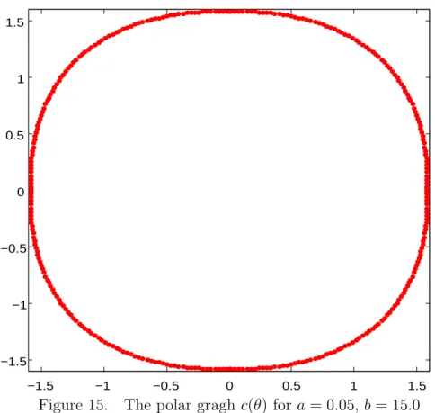
As θ less increase from θ = 0 to θ = π/2, we can obtain the following c − θ polar coordinate figure.
−1.5 −1 −0.5 0 0.5 1 1.5 −1.5 −1 −0.5 0 0.5 1 1.5
Figure 15. The polar gragh c(θ) for a = 0.05, b = 15.0
We set a = 0.1 and choose the particular angles, θ = 0, θ = π/4, and θ = π/2 to observe the convergence of numerical solutions for continuation method. Then the results we obtain are as follows.
−30 −2 −1 0 1 2 3 0.1 0.2 0.3 0.4 0.5 0.6 0.7 0.8 0.9 1 a = 0.1 b = 15.0 d1 = 1.0 d2 = 1.0 d3 = 4.4 d4 = 1.2 d5 = 1.2 a = 0.1 b = 15.0 d1 = 1.0 d2 = 1.0 d3 = 4.4 d4 = 1.2 d5 = 1.2 a = 0.1 b = 15.0 d1 = 1.0 d2 = 1.0 d3 = 4.4 d4 = 1.2 d5 = 1.2 a = 0.1 b = 15.0 d1 = 1.0 d2 = 1.0 d3 = 4.4 d4 = 1.2 d5 = 1.2 a = 0.1 b = 15.0 d1 = 1.0 d2 = 1.0 d3 = 4.4 d4 = 1.2 d5 = 1.2 a = 0.1 b = 15.0 d1 = 1.0 d2 = 1.0 d3 = 4.4 d4 = 1.2 d5 = 1.2 a = 0.1 b = 15.0 d1 = 1.0 d2 = 1.0 d3 = 4.4 d4 = 1.2 d5 = 1.2 a = 0.1 b = 15.0 d1 = 1.0 d2 = 1.0 d3 = 4.4 d4 = 1.2 d5 = 1.2 a = 0.1 b = 15.0 d1 = 1.0 d2 = 1.0 d3 = 4.4 d4 = 1.2 d5 = 1.2 Figure 16. θ = 0 −30 −2 −1 0 1 2 3 0.1 0.2 0.3 0.4 0.5 0.6 0.7 0.8 0.9 1 a = 0.1 b = 15.0 d1 = 1.0 d2 = 1.0 d3 = 4.4 d4 = 1.2 d5 = 1.2 a = 0.1 b = 15.0 d1 = 1.0 d2 = 1.0 d3 = 4.4 d4 = 1.2 d5 = 1.2 a = 0.1 b = 15.0 d1 = 1.0 d2 = 1.0 d3 = 4.4 d4 = 1.2 d5 = 1.2 a = 0.1 b = 15.0 d1 = 1.0 d2 = 1.0 d3 = 4.4 d4 = 1.2 d5 = 1.2 a = 0.1 b = 15.0 d1 = 1.0 d2 = 1.0 d3 = 4.4 d4 = 1.2 d5 = 1.2 a = 0.1 b = 15.0 d1 = 1.0 d2 = 1.0 d3 = 4.4 d4 = 1.2 d5 = 1.2 a = 0.1 b = 15.0 d1 = 1.0 d2 = 1.0 d3 = 4.4 d4 = 1.2 d5 = 1.2 a = 0.1 b = 15.0 d1 = 1.0 d2 = 1.0 d3 = 4.4 d4 = 1.2 d5 = 1.2 a = 0.1 b = 15.0 d1 = 1.0 d2 = 1.0 d3 = 4.4 d4 = 1.2 d5 = 1.2 Figure 17. θ = π/4
−30 −2 −1 0 1 2 3 0.1 0.2 0.3 0.4 0.5 0.6 0.7 0.8 0.9 1 a = 0.1 b = 15.0 d1 = 1.0 d2 = 1.0 d3 = 4.4 d4 = 1.2 d5 = 1.2 a = 0.1 b = 15.0 d1 = 1.0 d2 = 1.0 d3 = 4.4 d4 = 1.2 d5 = 1.2 a = 0.1 b = 15.0 d1 = 1.0 d2 = 1.0 d3 = 4.4 d4 = 1.2 d5 = 1.2 a = 0.1 b = 15.0 d1 = 1.0 d2 = 1.0 d3 = 4.4 d4 = 1.2 d5 = 1.2 a = 0.1 b = 15.0 d1 = 1.0 d2 = 1.0 d3 = 4.4 d4 = 1.2 d5 = 1.2 a = 0.1 b = 15.0 d1 = 1.0 d2 = 1.0 d3 = 4.4 d4 = 1.2 d5 = 1.2 a = 0.1 b = 15.0 d1 = 1.0 d2 = 1.0 d3 = 4.4 d4 = 1.2 d5 = 1.2 a = 0.1 b = 15.0 d1 = 1.0 d2 = 1.0 d3 = 4.4 d4 = 1.2 d5 = 1.2 a = 0.1 b = 15.0 d1 = 1.0 d2 = 1.0 d3 = 4.4 d4 = 1.2 d5 = 1.2 Figure 18. θ = π/2 Table 4. θ = 0, π/4, π/2 θ Converges ? α c 0 Yes 1.00 1.288 π/4 Yes 1.00 1.423 π/2 Yes 1.00 1.288
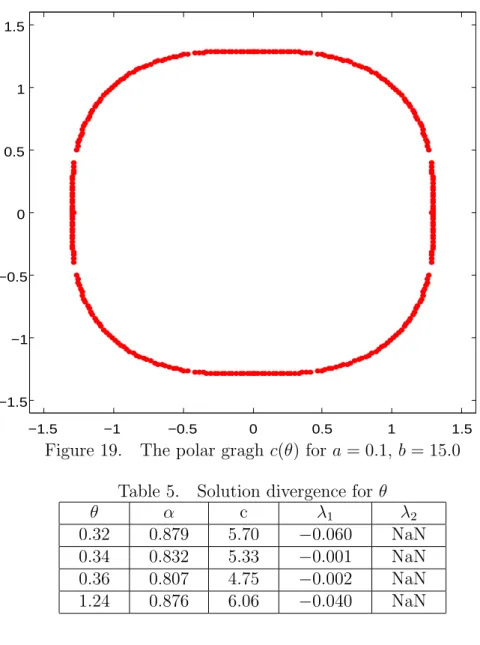
As θ less increase from θ = 0 to θ = π/2, we can obtain the following c − θ polar coordinate figure.
−1.5 −1 −0.5 0 0.5 1 1.5 −1.5 −1 −0.5 0 0.5 1 1.5
Figure 19. The polar gragh c(θ) for a = 0.1, b = 15.0 Table 5. Solution divergence for θ
θ α c λ1 λ2
0.32 0.879 5.70 −0.060 NaN 0.34 0.832 5.33 −0.001 NaN 0.36 0.807 4.75 −0.002 NaN 1.24 0.876 6.06 −0.040 NaN
Appendixes
A
The Algorithms
To indite our MATLAB program more conveniently, we use a pseudocode to describe the nested iteration scheme of continuation method containing the outer loop, secant method, for the wave speed c and Newton’s iteration which is during the inner loop. Here we attempt to approach the following one-parameter family of equations
c ˙ϕ(ξ) = fα(ϕ(ξ)) + d1g(ϕ(ξ − r1)) + d2g(ϕ(ξ − r2)) −
d3g(ϕ(ξ)) + d4g(ϕ(ξ + r1)) + d5g(ϕ(ξ + r2)),
with ϕ(−∞) = 0, ϕ(+∞) = 1,
fα(ϕ) = αf (ϕ) + (1 − α)fe(ϕ), 0 ≤ α ≤ 1,
where fe(ϕ) is given by (2.25).
The nonlinear system
F =
left-hand side of (2.23) for j = 0, 1, ..., (N2 − 1) ϕj − 0.5 for j = N/2
left-hand side of (2.23) for j = (N2 + 1), ..., N .
which is we are interesting to solve. For the continuation method, we use the following algorithms to solve the one-parameter family of equations and F = 0.
Algorithm 1: Continuation method.
Input: Initial guess Φ(0); Error accuracy acy;
Maximum number of iterations N1.
Output: Approximate solution Φ, wave speed c, or message of failure. Set α = 0 and c1 = 1.0.
while α ≤ 1 do Set c = c1.
Use Newton’s iteration to solve the system (2.24). Set h1 = h1(c, Φ).
(Note: hi(c, Φ) = left-hand side of (2.23) for j = N/2.)
if |h1| < acy then
Set c1 = c and Φ(0) = Φ.
else
Set c2 = c1+ 0.02.
Set c = c2.
Use Newton’s iteration to solve the system (2.24). Set h2 = h2(c, Φ).
if |h2| < acy then
Set c1 = c and Φ(0) = Φ.
else
Set i = 1. (Note: Solve the wave speed c by secant method.) while (i ≤ N1) do
Set c3 = c2− h2(c2 −c1) h2−h1 .
Set c = c3.
Use Newton’s iteration to solve the system (2.24). Set h3 = h3(c, Φ). if |h3| < acy then Set c1 = c and Φ(0) = Φ. STOP. else Set i = i + 1. if i > N1 then
STOP. (Note: Procedure failure.) end Set c1 = c2 and h1 = h2. Set c2 = c3 and h2 = h3. end end end end end
Algorithm 2: Newton’s iteration.
Input: Initial guess λ(0)1 , λ(0)2 , and Φ(0);
Error accuracy eps;
Maximum number of iterations N2.
Output: Approximate solution Φ; characteristic roots λ1 and λ2;
or failed message. if c < 0 then
STOP. (Note: Procedure failure.) else
Estimate the value of λ1 by 1-D Newton’s method.
if λ1 isn’t convergent or λ1 ≤ 0 then
STOP. (Note: Procedure failure.) else
Estimate the value of λ2 by 1-D Newton’s method.
if λ2 isn’t convergent or λ2 ≥ 0 then
STOP. (Note: Procedure failure.) else
Start high dimensional Newton’s iteration. Set index = 1.
while (index ≤ N2) do
Calculate F (Φ(0)) and the Jacobian matrix J (Φ(0))
to solve the (N + 1) × (N + 1) linear system J (Φ(0))Y = −F (Φ(0)). Set Φ(0) = Φ(0)+ Y . if kY k < eps then Set Φ = Φ(0). OUTPUT (Φ). STOP. else
Set index = index + 1. if index > N2 then
STOP. (Note: Procedure failure.) end end end end end end
B
Data of Polar Figures
B−1 Identity Map to Coupling g
Table A. a = 0.05, b = 15.0 θ converge ? α c λ1 λ2 0.000 Yes 1.00 1.371 2.26 −3.81 0.020 Yes 1.00 1.391 2.28 −3.80 0.080 Yes 1.00 1.381 2.27 −3.81 0.140 Yes 1.00 1.388 2.29 −3.83 0.220 Yes 1.00 1.394 2.32 −3.86 0.260 Yes 1.00 1.396 2.33 −3.89 0.280 Yes 1.00 1.400 2.35 −3.90 0.320 Yes 1.00 1.403 2.37 −3.93 0.360 Yes 1.00 1.408 2.39 −3.97 0.400 Yes 1.00 1.412 2.42 −4.00 0.440 Yes 1.00 1.421 2.45 −4.04 0.480 Yes 1.00 1.427 2.48 −4.08 0.500 Yes 1.00 1.430 2.49 −4.10 0.540 Yes 1.00 1.436 2.52 −4.14 0.580 Yes 1.00 1.439 2.55 −4.19 0.640 Yes 1.00 1.443 2.58 −4.24 0.660 Yes 1.00 1.449 2.60 −4.25 0.700 Yes 1.00 1.451 2.61 −4.28 0.780 Yes 1.00 1.453 2.63 −4.30 0.840 Yes 1.00 1.452 2.62 −4.29 0.900 Yes 1.00 1.450 2.60 −4.26 0.960 Yes 1.00 1.444 2.57 −4.21 1.000 Yes 1.00 1.439 2.54 −4.18 1.040 Yes 1.00 1.432 2.51 −4.14 1.080 Yes 1.00 1.427 2.48 −4.09 1.160 Yes 1.00 1.424 2.43 −4.01 1.180 Yes 1.00 1.415 2.41 −3.99 1.220 Yes 1.00 1.407 2.39 −3.96 1.280 Yes 1.00 1.401 2.35 −3.91 1.360 Yes 1.00 1.394 2.31 −3.86 1.440 Yes 1.00 1.388 2.29 −3.82 1.520 Yes 1.00 1.382 2.27 −3.81 1.571 Yes 1.00 1.382 2.27 −3.80
B−2 Hyper-Tangent Map to Coupling g Table E. a = 0.05, b = 15.0 θ converge ? α c λ1 λ2 0.000 Yes 1.00 1.371 2.26 −3.81 0.020 Yes 1.00 1.391 2.28 −3.80 0.080 Yes 1.00 1.381 2.27 −3.81 0.140 Yes 1.00 1.388 2.29 −3.83 0.220 Yes 1.00 1.394 2.32 −3.86 0.260 Yes 1.00 1.396 2.33 −3.89 0.280 Yes 1.00 1.400 2.35 −3.90 0.320 Yes 1.00 1.403 2.37 −3.93 0.360 Yes 1.00 1.408 2.39 −3.97 0.400 Yes 1.00 1.412 2.42 −4.00 0.440 Yes 1.00 1.421 2.45 −4.04 0.480 Yes 1.00 1.427 2.48 −4.08 0.500 Yes 1.00 1.430 2.49 −4.10 0.540 Yes 1.00 1.436 2.52 −4.14 0.580 Yes 1.00 1.439 2.55 −4.19 0.640 Yes 1.00 1.443 2.58 −4.24 0.660 Yes 1.00 1.449 2.60 −4.25 0.700 Yes 1.00 1.451 2.61 −4.28 0.780 Yes 1.00 1.453 2.63 −4.30 0.840 Yes 1.00 1.452 2.62 −4.29 0.900 Yes 1.00 1.450 2.60 −4.26 0.960 Yes 1.00 1.444 2.57 −4.21 1.000 Yes 1.00 1.439 2.54 −4.18 1.040 Yes 1.00 1.432 2.51 −4.14 1.080 Yes 1.00 1.427 2.48 −4.09 1.160 Yes 1.00 1.424 2.43 −4.01 1.180 Yes 1.00 1.415 2.41 −3.99 1.220 Yes 1.00 1.407 2.39 −3.96 1.280 Yes 1.00 1.401 2.35 −3.91 1.360 Yes 1.00 1.394 2.31 −3.86 1.440 Yes 1.00 1.388 2.29 −3.82 1.520 Yes 1.00 1.382 2.27 −3.81 1.571 Yes 1.00 1.382 2.27 −3.80
References
[1] Bates, P. W., and Chmaj, A. (1999). A discrete convolution model for phase transitions. Arch. Rational Mech. Anal. 150, 281-305.
[2] Bell, J. (1981). Some threshold results for models of Myelinated Nerves. Math. Biosci. 54, 181-190.
[3] Cahn, J. W. (1960), Theory of crystal growth and interface motion in crystalline materials. Acta Met. 8, 554-562.
[4] C. E. Elmer and E. S. Van Vleck, Computation of traveling waves for spatially discrete bistable reaction-diffusion equations, Applied Numer-ical Mathematics, 20 (1996), pp. 157-169.
[5] C.-H. Hsu and S.-S. Lin, Existence and multiplicity of traveling waves in a lattice dynamical system, J. Diff. Eqns., 164 (2000), pp. 431-450. [6] Chua, L. O. and Roska, T. (1993). The CNN paradigm. IEEE Trans.
Circuits Syst. 40, 147-156.
[7] E. Wasserstorm, Numerical solution by the continuation method, SIAM Review, 15 (1973), pp. 89-119.
[8] Erneux, T., and Nieolis, G. (1993). Propagating waves in discrete bistable reaction-diffusion systems. Physica D 67, 237-244.
[9] H. Chi, J. Bell, and B. Hassard, Numerical solution of a nonlinear ad-vance delay differential equation from nerve conduction theory, Journal of Mathematical Biology, 24 (1986), pp. 583-601.
[10] H. J. Hupkes and S. M. Verduyn Lunel, Analysis of Newton’s method to compute travelling waves in discrete media, Journal of Dynamics and Differential Equations, Vol. 17, No. 3, July 2005.
[11] J. Wu and X. Zou, Asymptotic and periodic boundary value problems of mixed FDEs and wave solutions of lattice differential equations, Journal of Differential Equations, 135 (1997), pp. 315-357.
[12] Keener, J., and Sneed, J. (1998). Mathematical Physiology. Springer-Verlag, New York.
[13] Laplante, J, P., and Erneux, T. (1992). Propagation failure in arrays of coupled bistable chemical reactors. J. Phys. Chem. 96, 4931-934.
[14] L. N. Trefethen, Finite Difference and Spectral Methods for Ordinary and Partial Differential Equations, Cornell University, 1996.
[15] L. O. Chua and L. Yang, Cellular neural networks: Theory, IEEE Trans. Circuits Syst., 35 (1988), pp. 1257-1272.
[16] L. O. Chua and L. Yang, Cellular neural networks: Applications, IEEE Trans. Circuits Syst., 35 (1988), pp. 1273-1290.
[17] P. W. Bates, X. Chen, and A. Chmaj, Traveling waves of bistable dy-namics on a lattice, SIAM J. Math. Anal., 35 (2003), pp. 520-546. [18] R. L. Burden and J. D. Faires, Numerical Analysis, 8th edition,
Brooks-Cole, 2005.
[19] S. Ma, X. Liao, and J. Wu, Traveling wave solutions for planar lattice differential systems with applications to neural networks, Journal of Differential Equations, 182 (2002), pp. 269-297.
[20] Y.-C. Lin, Numerical computation for traveling wave solutions of lattice differential equations, National Central University, 2005.