PALINDROMIC QUADRATIZATION AND
STRUCTURE-PRESERVING ALGORITHM FOR PALINDROMIC
MATRIX POLYNOMIALS OF EVEN DEGREE∗
TSUNG-MING HUANG†, WEN-WEI LIN‡, AND WEI-SHUO SU§
Abstract. In this paper, we mainly propose a palindromic quadratization to transform a dromic matrix polynomial of even degree into a palindromic quadratic pencil, instead of the palin-dromic linearization to a palinpalin-dromic linear pencil. Then, the structure-preserving algorithm for solving palindromic quadratic pencil based on (S + S−1)-transform and Patel’s algorithm 1993 can be applied directly to solve the palindromic matrix polynomial. Numerical experiments show that the backward errors for the palindromic polynomial eigenvalue problem computed by the palindromic quadratic pencil are better than that by palindromic linear pencil and the “polyeig” in MATLAB.
Key words. palindromic quadratization, palindromic matrix polynomial, palindromic quadratic pencil, structure-preserving algorithm
AMS subject classifications. 65F15, 15A18, 15A57
1. Introduction. In this paper, we consider (?, ε)-palindromic matrix polyno-mials of even degree 2d
P(λ) ≡ d−1 X j=0 λ2d−jA? d−j+ λdA0+ ε d X j=1 λd−jA j, (1.1)
where d ≥ 2, ε = ±1 and ? = H (Hermitian) or T (transpose), Aj ∈ Cn×n, for
j = 0, 1, . . . , d and A?
0 = εA0. The corresponding polynomial eigenvalue problem
P(λ)x = 0 with λ ∈ C and x ∈ Cn\{0} being the eigenvalue and the associated
eigenvector, respectively, is called a (?, ε)-palindromic polynomial eigenvalue problem ((?, ε)-PPEP). It is also called a ?-PPEP if ε = 1 or a ?-anti-PPEP if ε = −1.
The underlying matrix polynomial P(λ) in (1.1) has the property that revers-ing the order of coefficients, followed by takrevers-ing the (conjugate) transpose, leads to the original matrix polynomial (anti-)invariant, which explains the world “(anti-)palindromic”. Consequently, taking the (conjugate) transpose of (1.1), we easily see that eigenvalues of P(λ) satisfy a “reciprocal” property, that is, they are paired with respect to the unit circle, containing both eigenvalues λ and 1/λ?.
The (?, ε)-PPEPs arise in solving numerical solutions of higher order systems of ordinary or partial differential equations. A T-palindromic quadratic eigenvalue prob-lem (T-PQEP) is first raised in the study of the vibration in the structural analysis for fast trains in Germany [5, 6], and then of the behavior of periodic surface acous-tic wave filters [21]. A H-palindromic quadraacous-tic eigenvalue problem (H-PQEP) is raised in the computation of the Crawford number by bisection and level set methods for detecting a definite Hermitian pair and a hyperbolic or elliptic quadratic eigen-value problem [4]. A typical ?-PPEP of even degree is derived by solving the linear
∗Version June 22, 2009
†Department of Mathematics, National Taiwan Normal University, Taipei 116, Taiwan; [email protected].
‡Department of Applied Mathematics, National Chiao Tung University, Hsinchu 300, Taiwan; [email protected]
§Department of Applied Mathematics, National Chiao Tung University, Hsinchu 300, Taiwan; [email protected]
quadratic discrete-time optimal control problem subject to the higher order discrete system [1, 20].
A standard approach for solving the eigenpairs of P(λ) in (1.1) is to linearize P(λ) into a 2dn × 2dn linear matrix pencil by the companion linearization and compute its generalized Schur form (See e.g. [19]). However, the reciprocal property of eigenvalues of P(λ) is not preserved by computation, generally, producing large numerical errors ([3, 7, 8]). Recently, some pioneering works [12, 13] propose a good linearization of
P(λ) that linearizes it to a palindromic linear pencil λZ?+Z and preserves reciprocity
of eigenvalues. This does lead to a vast improvement over previous unstructured ap-proaches that reflects the palindromic structure in the original polynomial so that the structure-preserving numerical method can possibly be designed to leave the qualita-tive property of the spectrum intact. Later, a QR-like algorithm [16] and a hybrid method [11] which combines Jacobi-type method with the Laub’s trick, a postpro-cessing step of the generalized Schur form, are proposed for solving the T-palindromic linear pencil efficiently. The QR-like algorithm typically requires O(n4) flops and
the hybrid method requires O(n3log(n)) flops. Recently, a URV-decomposition based
structured method of cubic complexity is developed in [17] to solve the T-palindromic linear pencil, producing eigenvalues which are paired to working precision. On the other hand, for solving a (?, ε)-PQEP, a structure-preserving doubling algorithm is developed in [2, 3] via the computation of a solvent of a nonlinear matrix equation associated with the (?, ε)-PQEP. Lately, a numerically stable structure-preserving al-gorithm (SPA) based on the (S + S−1)-transform [10] and Patel’s algorithm [14] is proposed in [7] to solve the T-PQEP directly. The numerical results obtained by the SPA algorithm show much promise and the computational cost of SPA is about a half of that of the URV-based method.
The purpose of this paper is to develop a palindromic quadratization which quadratizes a (?, ε)-palindromic matrix polynomial of even degree with (?, ε) 6= (T, −1) into a (?, ε)-palindromic quadratic pencil. If ? = T and ε = 1, then we can apply the SPA algorithm in [7] to solve the associated quadratized T-PQEP directly. If ? = H and ε = ±1, we first transform the associated quadratized (H, ε)-PQEP to a H-skew-Hamiltonian pencil by the (S + S−1)-transform and enlarge the H-skew-Hamiltonian pencil to a real skew-Hamiltonian pencil, and then apply the SPA algorithm to solve it. Note that for the case (?, ε) = (T, −1) the T-anti-PPEP can then be solved by applying the URV-based method [15, 17] to the linearized T-palindromic linear pencil. Throughout this paper, Cn×mis the set of all n×m complex matrices, Cn = Cn×1 and C = C1. In and 0n×m (or simply I and 0 if their dimensions are clear from
the context) denote the n × n and n × m identity and zero matrices, respectively. Furthermore, 0n×m is the void if n = 0 or m = 0. The jth column of an identity matrix is denoted by ej. ⊕ and ⊗ denote the direct sum and the Kronecker product of two matrices, respectively.
This paper is organized as follows. In Section 2, we propose a palindromic quadra-tization to transform a (?, ε)-palindromic matrix polynomial of even degree into a (?, ε)-palindromic quadratic pencil. In Section 3, we develop a structure-preserving algorithm for solving the H-PQEPs. We derive backward error bounds and the diago-nal balance for PPEPs in Section 4 and 5, respectively. The comparisons of numerical results computed by the palindromic quadratization, the palindromic linearization and the standard companion linearization are presented in Section 6. Conclusions are given in Section 7.
2. P-Quadratization of (?, ε)-PPEP. Since the SPA algorithm in [7] is well-developed for solving a T-PQEP, it is motivated to propose a new palindromic quadra-tization (P-quadraquadra-tization) which can be utilized to quadratize a (?, ε)-PPEP into a (?, ε)-PQEP.
Definition 2.1.
(i) Let P(λ) be an n × n (?, ε)-palindromic matrix polynomial of degree 2d as in (1.1). A dn×dn (?, ε)-palindromic quadratic pencil Q(λ) ≡ λ2A?
1+λA0+εA1
with A?
0 = εA0 is called a P-quadratization of P(λ) if there are nonsingular
E(λ) and F(λ) with constant determinants such that E(λ)Q(λ)F(λ) = · P(λ) 0 0 I(d−1)n ¸ .
(ii) Generally, if C(λ) is an arbitrary n×n matrix polynomial of degree 2d, then a
dn × dn quadratic pencil D(λ) is a quadratization of C(λ) if there are nonsin-gular E(λ) and F(λ) with constant determinants such that E(λ)D(λ)F(λ) = diag(C(λ), I(d−1)n).
In general, there are infinitely many P-quadratizations Q(λ) for a given P(λ) in (1.1). However, unlike the unstructured linearization, the P-quadratization has much more constraints to be satisfied. In practice, it is not so easy to find a P-quadratization of P(λ). In the following theorem we shall give a “simplest” form (to our knowledge) of the P-quadratization Q(λ) for P(λ).
Theorem 2.2. A (?, ε)-palindromic matrix polynomial P(λ) in (1.1) with (?, ε) 6= (T, −1) can be P-quadratized into a (?, ε)-palindromic quadratic pencil of the form
Q(λ) ≡¡λ2A? 1+ λA0+ εA1 ¢ (2.1) with A? 0= εA0, where
(i) 2d = 4m: A1 and A0 are, respectively, given by
A1= A1 0n×(d−2)n d ? mIn ε√εd1A2m 0n×(d−2)n 0n A1,1 D1 0(d−2)n×n , (2.2a) A0= · A0− √ εIn− √ εA? 2mA2m A?0,1 εA0,1 D0 ¸ (2.2b) with A? 1,1= ½ ∅, if m = 1, £ A? 2m−1 0n A?2m−3 0n · · · A?3 0n ¤ , if m ≥ 2, D1= ½ ∅, if m = 1, diag¡d? 1In, −εd2In, d?2In, −εd3In, · · · , d?m−1In, −εdmIn ¢ , if m ≥ 2, A? 0,1= ½ 0n, if m = 1, £ 0n A? 2m−2 0n A?2m−4 0n · · · A?2 0n ¤ , if m ≥ 2, D0= ¡ −√εd1d?1In ¢ ⊕ 0(d−2)n;
(ii) 2d = 4m + 2: A1 and A0 are, respectively, given by
A1= · A1 0 d?mI A1,2 D2 0 ¸ , A0= · A0 A?0,2 εA0,2 0 ¸ (2.3) 3
with A?1,2= £ A? 2m+1 0 A?2m−1 0 · · · A?3 0 ¤ , D2= · 0 diag¡−εd1In, d?1In, · · · , −εdm−1In, d?m−1In, −εdmIn ¢ ¸ , A? 0,2= £ A? 2m 0 A?2m−2 0 · · · A?2 0 ¤ ;
in which d1, . . . , dm are arbitrary nonzero constants.
Proof. (i) for 2d = 4m: Let F1(λ) = · In F2,1(λ)T F3,1(λ)T · · · F2m,1(λ)T 0 I(2m−1)n ¸T . (2.4)
We first determine F2,1(λ), . . . , F2m,1(λ) so that
Q(λ)F1(λ) · In 0 ¸ = · Q1(λ) 0 ¸ (2.5) with Q1(λ) ∈ Cn×n. Substituting Q(λ) in (2.1) and (2.2) into (2.5), we have
0 = Q1(λ) − £ λ2A? 1+ λ ¡ A0− √ εIn− √ εA? 2mA2m ¢ + εA1+ λ2 √ εd? 1A?2mF2,1(λ) + m−1X k=1 ¡ λ2A?2m−2k+1+ λA?2m−2k ¢ F2k+1,1(λ) + εd?mF2m,1(λ) # , (2.6a) 0 =√εA2m− λ √ εd? 1F2,1(λ) + λ2F3,1(λ), (2.6b) 0 = (λ2d? j)F2j,1(λ) − ¡ d? j−1F2j−2,1(λ) + λA2m−2j+2+ A2m−2j+3 ¢ , for j = 2, . . . , m, (2.6c) 0 = F2j+1,1(λ) − λ2F2j+3,1(λ), for j = 1, . . . , m − 2, (2.6d) 0 = F2m−1,1(λ) − λ2In. (2.6e)
Substituting (2.6e) into (2.6d), it holds that
F2j+1,1(λ) = λ2F2j+3,1(λ) = λ2m−2jIn, for j = 1, . . . , m − 2. (2.7a) Substituting (2.7a) with j = 1 into (2.6b), it holds that
F2,1(λ) = (λd?1)−1 ¡ ε√ελ2mI n+ A2m ¢ . (2.7b)
Substituting (2.7b) into (2.6c) and using mathematical induction, we conclude that
F2j,1(λ) = ¡ λ2j−1d?j ¢−1Ã ε√ελ2mIn+ 2j−2X k=0 λkA2m−k ! , (2.7c)
for j = 2, . . . , m. Substituting (2.7a), (2.7b) and (2.7c) with j = m into (2.6a), we get
Q1(λ) = λ1−2mP(λ). (2.8)
Similarly, we see that the matrix
E1(λ) = · In E1,2(λ) E1,3(λ) · · · E1,2m(λ) 0 I(2m−1)n ¸ (2.9a)
with E1,2j(λ) = ¡ λ2m−2j+1d j ¢−1 Ã2j−2 X k=0 λ2m−kA? 2m−k+ √ εIn ! , for j = 1, . . . , m, (2.9b) E1,2j+1(λ) = λ2j−2mIn, for j = 1, . . . , m − 1 (2.9c) satisfies E1(λ)Q(λ)F1(λ) = λ1−2mP(λ) 0 0 0 · · · 0 0 Q22(λ) Q23(λ) 0 0 0 Q32(λ) 0 Q34(λ) . .. ... 0 0 Q43(λ) . .. . .. 0 .. . . .. . .. 0 Q2m−1,2m(λ) 0 0 · · · 0 Q2m,2m−1(λ) 0 , where Q22(λ) = −λ√εd1d?1In and Q`,`+1(λ) = λ2d iIn, Q`+1,`+2(λ) = −λ2εd?i+1In, Q`+1,`(λ) = εd?iIn, Q`+2,`+1(λ) = −di+1In, for ` = 2i and i = 1, . . . , m − 1.
From facts that " In 0 √ ε λdiIn In # · −λ√εdid?iIn Q`,`+1(λ) Q`+1,`(λ) 0 ¸ " In √εdλ? iIn 0 In # = · −λ√εdid?iIn 0 0 λ√εIn ¸ and " In 0 di+1 √ ελIn In # · λ√εIn Q`+1,`+2(λ) Q`+2,`+1(λ) 0 ¸ · In λ√εd?i+1In 0 In ¸ = · λ√εIn 0 0 −λ√εdi+1d?i+1In ¸
for ` = 2i and i = 1, . . . , m − 1, we have
E2m−1(λ) · · · E2(λ)E1(λ)Q(λ)F1(λ)F2(λ) · · · F2m−1(λ) = diag¡λ1−2mP(λ), −λ√εd1d?1In, λ √ εIn, · · · , λ √ εIn, −λ √ εdmd?mIn ¢ , where E2i(λ) = I(2i−1)n⊕ " In 0 √ ε λdiIn In # ⊕ I(2m−2i−1)n, (2.10a) E2i+1(λ) = I2in⊕ " In 0 d√i+1 ελIn In # ⊕ I(2m−2i−2)n, (2.10b) 5
for i = 1, 2, . . . , m − 1, and F2i(λ) = I(2i−1)n⊕ " In √λεd? iIn 0 In # ⊕ I(2m−2i−1)n, (2.11a) F2i+1(λ) = I2in⊕ · In λ √ εd? i+1In 0 In ¸ ⊕ I(2m−2i−2)n, (2.11b)
for i = 1, . . . , m − 1. Finally, letting
E2m(λ) = diag ¡ λ2m−1In, −(λ √ εd1d?1)−1In, (λ √ ε)−1In, −(λ √ εd2d?2)−1In, · · · , (λ√ε)−1I n, −(λ √ εdmd?m)−1In ¢ , (2.12)
we have that E(λ)Q(λ)F(λ) = diag(P(λ), I(2m−1)n), where E(λ) = E2m(λ) · · · E1(λ)
and F(λ) = F1(λ) · · · F2m−1(λ).
(ii) for 2d = 4m + 2: Let Π2i= I(2i−1)n⊕ · 0 In In 0 ¸ ⊕ I(2m−2i), for i = 1, . . . , m.
Similar to part (i), we see that
E1(λ) = Π2 · In E1,2(λ) E1,3(λ) · · · E1,2m+1(λ) 0 I2mn ¸ , (2.13a) F1(λ) = · In F2,1(λ)T F3,1(λ)T · · · F2m+1,1(λ)T 0 I2mn ¸T (2.13b) with E1,2j(λ) = λ2j−2m−2In, E1,2j+1(λ) = d−1j 2j−1X k=0 λk+1A? 2m+k−2j+2, (2.13c) F2j,1(λ) = λ2m−2j+2In, F2j+1,1(λ) = ¡ d?jλ2j ¢−12j−1X k=0 λkA2m−k+1 (2.13d) for j = 1, . . . , m, satisfy Q(λ)F1(λ) · In 0 ¸ = · λ−2mP(λ) 0 ¸ (2.14) and £ In 0 ¤ E1(λ)Q(λ)F1(λ) = £ λ−2mP(λ) 0 ¤. Letting Ei(λ) = Π2i µ I2(i−1)n⊕ · In 0 λ−2I n In ¸ ⊕ I(2m−2i+1)n ¶ , (2.15a) Fi(λ) = I(2i−3)n⊕ In 0 λ 2I n 0 In In 0 0 In ⊕ I(2m−2i+1)n, (2.15b)
for i = 2, . . . , m, and Em+1(λ) = diag µ λ2mI n,−1 d1 In, −1 λ2εd? 1 In,−1 d2 In, −1 λ2εd? 2 In, · · · ,−1 dm In, −1 λ2εd? m In ¶ , (2.16) one can also verify that E(λ)Q(λ)F(λ) = diag(P(λ), I2mn), where E(λ) = Em+1(λ) · · · E1(λ)
and F(λ) = F1(λ) · · · Fm(λ).
Note that the P-quadratization of a (?, ε)-palindromic matrix polynomial of odd degree with even matrix dimension can also be defined as in Definition 2.1, however, to our knowledge, it is difficult to find a solution for this type of P-quadratization.
We now show the relationship between the eigenvectors of Q(λ) and P(λ). Theorem 2.3. Let Q(λ) in (2.1) be the P-quadratization of P(λ) in (1.1) with (?, ε) 6= (T, −1). If (λ, y) with y =£ yT
1 · · · yTd ¤T
and yi ∈ Cn, i = 1, . . . , d, is
an eigenpair of Q(λ), then (λ, y1) is an eigenpair of P(λ) and {yi}2mi=1 satisfy that (i) for 2d = 4m: ( y2j= ¡ d? jλ2j−1 ¢−1³ ε√ελ2mI +P2j−2 i=0 λiA2m−i ´ y1, for j = 1, . . . , m, y2j+1= λ2m−2jy1, for j = 1, . . . , m − 1; (ii) for 2d = 4m + 2: ( y2j = λ2m−2j+2y1, for j = 1, . . . , m, y2j+1= ¡ d? jλ2j ¢−1³P2j−1 i=0 λiA2m−i+1 ´ y1, for j = 1, . . . , m.
Proof. Since Q(λ) is a P-quadratization of P(λ) and (λ, y) is an eigenpair of Q(λ),
by Theorem 2.2 there are nonsingular E(λ) and F(λ) such that 0 = Q(λ)y = E(λ)−1diag(P(λ), I
(d−1)n)F(λ)−1y.
This implies that diag(P(λ), I(d−1)n)F(λ)−1y = 0. Hence, y = F(λ)
· ˜ y1 0 ¸ with
P(λ)˜y1= 0. By the definition of F(λ) in (2.4) and (2.11) for 2d = 4m or (2.13b) and
(2.15b) for 2d = 4m + 2, we have y = F1(λ) · ˜ y1 0 ¸ = ˜ y1 F2,1(λ)˜y1 .. . Fd,1(λ)˜y1 . (2.17)
This proves the assertions (i) and (ii) of the theorem by substituting (2.7) and (2.13d), respectively, into (2.17).
As mentioned before, there are infinitely many P-quadratizations of P(λ) as in (1.1). Theorem 2.2 gives a way for finding a P-quadratization for (1.1). As in [12, 13], for a given P(λ) in (1.1), a P-quadratization Q(λ) of P(λ) can be obtained by finding a nonzero h ∈ Cd and H(λ) ∈ Cdn×n with degree 2d − 2 such that
Q(λ)H(λ) = h ⊗ P(λ), (2.18)
where Q(λ) is a dn × dn (?, ε)-palindromic quadratic pencil. If z ∈ Cdn\{0} is a left eigenvector of Q(λ), we then have 0 = zTQ(λ)H(λ) = zT(h⊗P(λ)) = zT(h⊗In)P(λ). Thus zT(h ⊗ In) is a left eigenvector of P(λ).
Similarly, a P-quadratization Q(λ) of P(λ) can also be solved by finding a nonzero
g ∈ Cd and G(λ) ∈ Cn×dn with degree 2d − 2 such that
G(λ)Q(λ) = gT ⊗ P(λ). (2.19)
If y ∈ Cdn\{0} is a right eigenvector of Q(λ), then we have 0 = G(λ)Q(λ)y =
gT⊗ P(λ)y = P(λ)(gT⊗ In)y. Thus, (gT ⊗ In)y is a right eigenvector of P(λ).
The P-quadratization Q(λ) defined in (2.1) must satisfy (2.18) and (2.19), respec-tively. In fact, for the case 2d = 4m, from (2.5) and (2.8), we define h = e1 ∈ Cd
and H(λ) =£λ2m−1I
n, λ2m−1F2,1(λ)T, · · · , λ2m−1F2m,1(λ)T
¤T
which satisfies (2.18) with Q(λ) being defined in (2.1) and (2.2). For the case 2d = 4m + 2, from (2.14), we define h = e1 ∈ Cd and H(λ) = £ λ2mI n, λ2mF2,1(λ)T, · · · , λ2mF2m+1,1(λ)T ¤T which satisfies (2.18) with Q(λ) being defined in (2.1) and (2.3).
To show that (2.19) holds for both cases 2d = 4m and 4m + 2, by the palindromic property of P(λ) and taking h = e1, we have that Q?(λ) (H?(λ))T = ed⊗P?(λ). This
implies that HT(λ)Q(λ) = eT
d ⊗ P(λ) which satisfies (2.19).
Remark 2.1. (i) Theorem 2.2 cannot be applied to the case when (?, ε) = (T, −1).
In fact, up to now, there is no structure-preserving algorithm to solve a T-anti-PQEP directly. So, it is useless to transform a T-anti-PPEP to a T-anti-PQEP. Thus, for a (T, −1)-palindromic matrix polynomial we can apply the palindromic linearization
[12] to transform it into a T-palindromic linear pencil λZT + Z, and then use
QR-like algorithm [16], hybrid method [11] or the URV-based method [17] to solve its eigenpairs.
(ii) On the other hand, if we rewrite λZT+ Z to a T-palindromic quadratic pencil b
Q(bλ) ≡ bλ2ZT+ bλ0 + Z by letting bλ2= λ, then the SPA algorithm [7] can also be used
to solve its eigenpairs. It is shown in [7] that applying the SPA to solve bQ(bλ)y = 0 is
mathematically equivalent to applying the URV-based method to solve λZT + Z.
The following relationship between an H-anti-PQEP and H-PQEP can be easily obtained by setting λ = ıω and the fact (ıA0)H = ıA0.
Proposition 2.4. Given an H-anti-PQEP: (λ2AH
1 + λA0− A1)x = 0, with
AH
0 = −A0. Then (ıω, x) is an eigenpair of H-anti-PQEP if and only if (ω, x) is an
eigenpair of the H-PQEP:£ω2(−A
1)H+ ω(ıA0) + (−A1)
¤
x = 0.
We now consider the ?-even and ?-odd polynomial eigenvalue problems of even degree. Let C(λ) =P2di=0λiCi, where Ci∈ Cn×nfor i = 0, 1, . . . , 2d and C
2d6= 0. The
polynomial eigenvalue problem C(λ)x = 0 is called a ?-even polynomial eigenvalue problem, if C?
2i = C2i, i = 0, 1, . . . , d and C2i−1? = −C2i−1, i = 1, . . . , d; and it is
called a ?-odd polynomial eigenvalue problem, if C?
2i = −C2i, i = 0, 1, . . . , d and
C?
2i−1= C2i−1, i = 1, . . . , d. By the Cayley transformation, it was shown in [12] that
a ?-even/odd polynomial eigenvalue problem can be transformed to a (?, +1/ − 1)-PPEP, respectively.
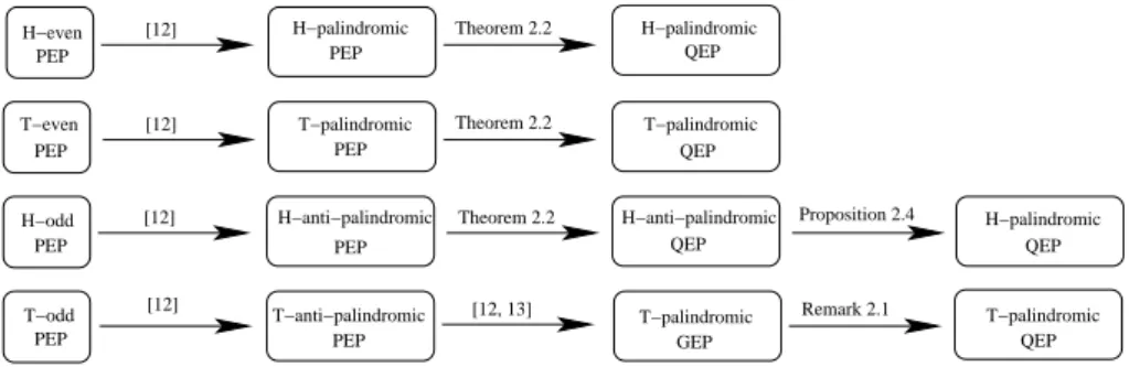
We illustrate the relationship among various structured polynomial eigenvalue problems in Figure 2.1. We see that even, odd, anti-palindromic and T-palindromic polynomial eigenvalue problems of even degree can be P-quadratized to T-PQEPs. Thus, the SPA algorithm in [7] can be applied to solve the associated T-PQEPs. On the other hand, we see that H-even, H-odd, H-anti-palindromic and H-palindromic polynomial eigenvalue problems of even degree can be P-quadratized to H-PQEPs. Therefore, it is motivated to develop a structure-preserving algorithm in the next section for solving the H-PQEP.
H−even PEP H−palindromic PEP T−even PEP PEP T−palindromic PEP H−anti−palindromic PEP H−palindromic QEP T−palindromic QEP H−anti−palindromic QEP H−palindromic QEP H−odd T−odd PEP T−palindromic QEP T−palindromic GEP PEP T−anti−palindromic [12, 13] [12] [12] [12] [12] Theorem 2.2 Theorem 2.2 Theorem 2.2 Remark 2.1 Proposition 2.4
Fig. 2.1. Relations between various structured polynomial eigenvalue problems (PEPs).
3. H-palindromic quadratic eigenvalue problems. Consider the H-PQEP
Q(λ)x ≡ (λ2AH1 + λA0+ A1)x = 0, (3.1)
where A0, A1 ∈ Cn×n with AH0 = A0. Taking the conjugate transpose of (3.1), we
easily see that the eigenvalues of Q(λ) have a “reciprocal” property, that is, they are paired with respect to the unit circle, containing both eigenvalues λ and its conjugate reciprocal 1/¯λ.
Classical linearizations of (3.1) in a companion form, generally, do not preserve the symplectic structure. Fortunately, the special linearization of (3.1) (see [2] or [7])
(M − λL)z ≡ µ· A1 0 −A0 −I ¸ − λ · 0 I AH 1 0 ¸¶ · x y ¸ = 0 (3.2) satisfies MJ MH= LJ LH (3.3)
which preserves reciprocity, where J ≡ J2n is the 2n × 2n matrix
·
0 In
−In 0
¸ . A pencil M − λL or the matrix pair (M, L) is called H-symplectic.
For any real symplectic matrix pair (M, L) satisfying (3.3), a structure-preserving (S + S−1)-transform for the computation of all eigenvalues was proposed by [10]. For a H-symplectic matrix pair (M, L), the (S + S−1)-transform (Ms, Ls) is defined by
Ms≡ MJ LH+ LJ MH≡ KJ , Ls≡ LJ LH ≡ N J . (3.4)
It is easily seen that K and N are both H-skew-Hamiltonian, i.e., KJ = J KH and
N J = J NH. Hence, if µ is an eigenvalue of (K, N ), so is ¯µ.
We first give the relationship between eigenpairs of a H-symplectic matrix pair and its (S + S−1)-transform.
Theorem 3.1. Let (M, L) be H-symplectic and (Ms, Ls) be its (S + S−1
)-transform as in (3.4). Suppose zs is an eigenvector of (Ms, Ls) corresponding to
µ = ν +1
ν. If (LH−ν1MH)zs6= 0 or (LH− νMH)zs6= 0, then (ν, J (LH−1νMH)zs)
or (1/ν, J (LH− νMH)zs), respectively, is an eigenpair of (M, L).
Proof. As in [10], since MJ MH= LJ LH, by (3.4) it holds that 0 = [Ms− µLs] zs= · MJ LH+ LJ MH− (ν + 1 ν)LJ L H ¸ zs = (M − νL)J (LH−1 νM H)zs (3.5a) = (M − 1 νL)J (L H− νMH)zs. (3.5b) By applying (3.5a), if (LH−1 νMH)zs6= 0, then J (LH−1νMH)zs is an eigenvector of (M, L) corresponding to ν. By applying (3.5b), if (LH − νMH)zs 6= 0, then
J (LH− νMH)zsis an eigenvector of (M, L) corresponding to 1/ν.
Let(M, L) be of the form in (3.2). We give the relationship between eigenpairs of (Ms, Ls) and Q(λ).
Theorem 3.2. Let (M, L) be H-symplectic of the form in (3.2) and (Ms, Ls)
be its (S + S−1)-transform. Define z
s≡ [zs1T, zTs2]T with zs1, zs2∈ Cn. Suppose that
zs is an eigenvector of (Ms, Ls) corresponding to the eigenvalue µ 6= ±2. Let ν be a
root of the quadratic equation λ + 1
λ = µ. Then: (i) at least one of vectors zs1+1
νzs2 and zs1+ νzs2 is nonzero; (ii) if zs1+1
νzs26= 0, then zs1+1νzs2 is an eigenvector of Q(λ) corresponding to ν; (iii) if zs1+1
νzs2= 0, then zs2 is an eigenvector of Q(λ) corresponding to 1ν.
Proof. (i) Suppose that zs1+ 1νzs2 = 0 and zs1+ νzs2 = 0. It implies that
(ν − 1
ν)zs2 = 0. If zs2 = 0, then zs1 = 0 and zs = 0 which contradicts that zs is an eigenvector. Hence, ν = ±1 and then µ = ±2 which contradicts that µ 6= ±2. Therefore, zs1+1
νzs26= 0 or zs1+ νzs26= 0. (ii). From (3.5a), it follows that
(M − νL) · zs1+ν1zs2 xν ¸ = 0, (3.6) where xν ≡ 1 νA H 1 zs1− 1 νA0zs2− A1zs2. (3.7)
Substituting (M, L) of (3.2) into (3.6), we have
xν = 1 νA1(zs1+ 1 νzs2) (3.8a) and A0(zs1+1 νzs2) + xν+ νA H 1 (zs1+ 1 νzs2) = 0. (3.8b)
Substituting xν in (3.8a) into (3.8b) and multiplying (3.8b) by ν we get
Q(ν)(zs1+1
νzs2) = 0.
(iii) Since zs1+1
νzs2= 0, it follows that zs1= −1νzs26= 0. From (3.8a) and (3.7), it holds that 0 = xν = − µ 1 ν ¶2 AH 1zs2−1 νA0zs2− A1zs2.
Therefore, zs2is an eigenvector of Q(λ) corresponding to the eigenvalue 1
ν.
In [7], a structure-preserving algorithm (SPA) based on Patel’s algorithm [14] is developed for solving T-PQEPs. In order to solve an H-PQEP, we apply the (S +S−1 )-transform to the H-symplectic pair (M, L) of the form (3.2) and get the generalized eigenvalue problem Kzs= µN zs, where
K = · A0 AH1 − A1 A1− AH1 A0 ¸ , N = · −A1 0 0 −AH 1 ¸ (3.9)
are H-skew-Hamiltonian. However, Patel’s algorithm can only be used to solve (K, N ) of (3.9) in the real case, but cannot be directly applied to solve (K, N ) in the complex conjugate case. In the following, we convert (K, N ) of (3.9) into an enlarged real T-skew-Hamiltonian pair so that Patel’s algorithm can be applied. We extend (K, N ) in (3.9) to a real 4n × 4n matrix pair (K2, N2) by
K2= · KR −KI KI KR ¸ , N2= · NR −NI NI NR ¸ ∈ R4n×4n, (3.10)
where K = KR+ ıKI and N = NR+ ıNI. From (3.10) it is easily seen that if µ is an eigenvalue of (K, N ), then µ and ¯µ are eigenvalues of (K2, N2).
Theorem 3.3. The multiplicities of eigenvalues of (K2, N2) are all even.
Proof. Write A0 = A0R+ ıA0I and A1 = A1R+ ıA1I with AT0R = A0R and
AT 0I = −A0I. Define e K2≡ ΠK2Π, Ne2≡ ΠN2Π, (3.11) where Π = In⊕ · 0 In In 0 ¸
⊕ In. Then, from (3.9), it is easy to check that eK2 and
e
N2 are real skew-Hamiltonian, i.e., ( eK2J4n)T = − eK2J4n and ( eN2J4n)T = − eN2J4n.
Therefore, from the result of [10] it follows that the multiplicities of eigenvalues of ( eK2, eN2) are all even.
From (3.4), we see that µ is an eigenvalue of (K, N ) if and only if ¯µ is an eigenvalue
of (K, N ). We now give the relationship between eigenpairs of (K, N ) and (K2, N2).
Theorem 3.4.
(i) If x+ıy is an eigenvector of (K, N ) corresponding to α+ıβ, then · x y ¸ ±ı · y −x ¸ is an eigenvector of (K2, N2) corresponding to α ± ıβ. (ii) If · x1 x2 ¸ + ı · y1 y2 ¸
is an eigenvector of (K2, N2) corresponding to α + ıβ, then
(x1− y2) + ı(x2+ y1) is an eigenvector of (K, N ) corresponding to α + ıβ.
Proof. The assertion (i) follows from (3.10) immediately. To prove (ii), by letting
x = x1− y2, y = x2+ y1and from (3.10) and assumption, we get
KRx − KIy = α(NRx − NIy) − β(NIx + NRy),
KIx + KRy = β(NRx − NIy) + α(NIx + NRy). Thus, x + ıy is an eigenvector of (K, N ) corresponding to α + ıβ.
From Theorems 3.3 and 3.4, the eigenpairs of (K, N ) can be computed from the eigenpairs of ( eK2, eN2) where eK2 and eN2 are defined in (3.11). Since eK2 and eN2 are
both real skew-Hamiltonian, based on Patel’s approach [7, 14], the pair ( eK2, eN2) can 11
be reduced to block upper triangular forms e K2:= QTKe2Z = · K11 K12 0 KT 11 ¸ , Ne2:= QTNe2Z = · N11 N12 0 NT 11 ¸ , (3.12) where Q, Z ∈ R4n×4nare orthogonal satisfying Q = JT
4nZJ4n, and K11, N11∈ R2n×2n
are upper Hessenberg and upper triangular, respectively.
From Theorem 3.3 and (3.12), we see that the pair (K11, N11) has the same
spec-trum as ( eK2, eN2). We then apply the QZ algorithm to (K11, N11) for computing
all eigenpairs {(µj, ˜zj)}2n j=1. Consequently, {(µj, ΠZ · ˜ zj 0 ¸ )}2n j=1 are 2n eigenpairs of (K2, N2), where Π is defined as in (3.11). Let µj = αj+ ıβj and ΠZ[˜zTj, 0T]T ≡ £ xT 1j, xT2j ¤T + ı£yT 1j, y2jT ¤T
with αj, βj ∈ R and x1j, x2j, y1j, y2j ∈ R2n. From
Theo-rem 3.4, {(αj+ıβj, JT(x
1j−y2j+ı(x2j+y1j)))}2nj=1are eigenpairs of (Ms, Ls). Finally, we compute all eigenvalues and the associated eigenvectors of Q(λ) by Theorem 3.2.
Algorithm 3.1 (Structure-Preserving Algorithm (SPA) for H-PQEP).
Input: A H-palindromic quadratic pencil Q(λ) ≡ λ2AH
1 + λA0+ A1 with
A0, A1∈ Cn×n and AH0 = A0;
Output: All eigenvalues and eigenvectors of Q(λ). Step 1. Form the matrix pair ( eK2, eN2) as in (3.11);
Step 2. Reduce ( eK2, eN2) to block upper triangular forms as in (3.12);
Step 3. Compute eigenpairs {(µj, ˜zj)}2nj=1 of (K11, N11) defined in (3.12)
by the QZ algorithm; Step 4. Compute ΠZ · ˜ zj 0 ¸ ≡ · x1j x2j ¸ + ı · y1j y2j ¸ , j = 1, 2, . . . , 2n;
Step 5. Compute the eigenpair (µj, zj), for j = 1, 2, . . . , 2n, of (Ms, Ls) by
zj = JT(x1j− y2j+ ı(x2j+ y1j)) ≡ [zj1T, zj2T]T;
Step 6. Compute νj and ν1j by solving ν2− µjν + 1 = 0;
Compute xj1≡ zj1+ν1jzj2 and xj2≡ zj1+ νjzj2for j = 1, 2, . . . , 2n; Step 7. If xj16= 0, then it is an eigenvector of Q(λ) corresponding to νj;
If xj26= 0, then it is an eigenvector of Q(λ) corresponding to ν1j;
4. Backward error analysis. Let (λ, x) be an approximate eigenpair of P(λ) as in (1.1). We define the backward error of (λ, x) by
η(λ, x) := hP kP(λ)xk
d
j=1(|λ|d+j+ |λ|d−j) kAjk + |λ|dkA0k
i
kxk
essentially as in [18] which minimizes the upper bound over all possible perturbations of coefficient matrices of P(λ). Recently, a structured backward error analysis of (λ, x) is discussed in [9] which proposed a computable formula for the optimal structured backward errors. In this section, we shall study the relationship between the residuals
r ≡ Q(λ)y and P2d(λ)y1 for a given approximate eigenpair (λ, y ≡ [yT1, · · · , yTd]T) of
Q(λ), where Q(λ) is a P-quadratization of P(λ) given in Theorem 2.2. This
relation-ship can be used to determine the parameters d1, . . . , dm in (2.2) and (2.3) for the reduction of the backward error.
Theorem 4.1. Let (λ, y ≡ [yT
1, · · · , ydT]T) be an approximate eigenpair of Q(λ)
in (2.1) associated with the residual r ≡ [rT
(i) for 2d = 4m: we have P4m(λ)y1= m X i=1 λ2i−2d−1 i 2i−2X j=0 λ2m−jA? 2m−j+ √ εI r2i +λ2m−1 m−1X i=1 λ2i−2mr 2i+1+ λ2m−1r1; (4.1)
(ii) for 2d = 4m + 2: we have
P4m+2(λ)y1= λ2m+1 m X i=1 d−1i 2i−1X j=0 λj+1A?2m+j−2i+2 r2i+1 + m X i=1 λ2i−2r2i+ λ2mr1. (4.2)
Proof. Since Q(λ) is a P-quadratization of P(λ), from Theorem 2.2 there are
nonsingular matrices E1(λ), . . . , Eν(λ) and F1(λ), . . . , Fν−1(λ) such that
Eν(λ) · · · E1(λ)Q(λ) = diag ¡ P(λ), I(d−1)n ¢ Fν−1(λ)−1· · · F 1(λ)−1, (4.3)
where ν = 2m, if 2d = 4m and ν = m + 1, if 2d = 4m + 2. By assumption that
r = Q(λ)y and using (4.3), it holds that
£ In 0 ¤ Eν(λ) · · · E1(λ)r = £ P(λ) 0 ¤Fν−1(λ)−1· · · F 1(λ)−1y. (4.4)
From F1(λ), . . . , Fν−1(λ) defined in (2.4) and (2.11) for 2d = 4m or defined in (2.13b)
and (2.15b) for 2d = 4m + 2, we have £
P(λ) 0 ¤Fν−1(λ)−1· · · F
1(λ)−1y = P(λ)y1. (4.5)
From E1(λ), . . . , Eν(λ) defined in (2.9)-(2.10) and (2.12) for 2d = 4m or defined in
(2.13a), (2.15a) and (2.16) for 2d = 4m + 2, we have £ In 0 ¤ Eν(λ) · · · E1(λ)r =£ In 0 ¤ Eν(λ) · In 0 ¸ (r1+ E1,2(λ)r2+ E1,3(λ)r3+ · · · + E1,d(λ)rd) . (4.6)
Substituting (2.9) and (2.13c), respectively, into (4.6) and using (4.4) and (4.5), it follows the results of (i) and (ii).
5. Balancing for P(λ) and Q(λ). Scaling is a commonly used technique for standard eigenvalue problems to improve the sensitivity of the eigenvalues. In this section, we first propose a diagonal scaling for P(λ) in (1.1). Then, we determine the free parameters d1, . . . , dmin (2.2) and (2.3) so that the backward errors of eigenpairs for P(λ) are improved and the entries of coefficient matrices in Q(λ) are balanced.
5.1. Balancing for P(λ) in (1.1). In order to balance the entries of coefficient matrices in P(λ), we define a complex diagonal matrix
D ≡ diag(2α1, 2α2+ıβ2, · · · , 2αn+ıβn)
with αi, βi ∈ R so that the magnitudes of entries of coefficient matrices in the new (?, ε)-palindromic matrix polynomial
D d−1 X j=0 λ2d−jA?d−j+ λdA0+ ε d X j=1 λd−jAj D?
are close to one as much as possible. That is, we shall determine α1, . . . , αn and
β2, . . . , βn so that
2αj+ıβjAk(j, `)2α`−ıβ` ≈ 1, (5.1)
for j, ` = 1, 2, . . . , n and k = 0, 1, . . . , d, where Ak(j, `) is the (j, `)-th entry of Ak. By taking logarithm of (5.1), the parameters, α1, . . . , αnand β2, . . . , βncan be determined by solving the least square problems
αj+ α`= −Re(log2(Ak(j, `))), βj− β`= −Im(log2(Ak(j, `))),
where Re(c) and Im(c) represent the real and the imaginary parts of c, respectively. Then, the parameters α1, . . . , αn are solved by the normal equation
BTB [α
1, · · · , αn]T = BTb,
where b ≡ [bµ] with µ = kn2+ (j − 1)n + ` and bµ = −Re(log
2(Ak(j, `))), BTB is
invertible and (BTB)−1≡ [ˆb
ij] with ˆbij = −(2d + 1)/δ, if i 6= j and ˆbii= (4dn + 2n − 2d + 1)/δ with δ = b2
11+ (n − 2)b11b12− (n − 1)b2126= 0.
Similarly, the parameters β2, . . . , βn are solved by the normal equation
CTC [β
2, · · · , βn]T = CTc,
where c ≡ [cµ] with µ = kn2+ (j − 1)n + ` and cµ = −Im(log
2(Ak(j, `))), CTC
is invertible and (CTC)−1 ≡ [ˆc
ij] with ˆcij = 1/(n(2d + 1)), if i 6= j and ˆcii = 2/(n(2d + 1)).
Note that it only requires O(n2) flops to determine the diagonal matrix D.
5.2. Balancing for Q(λ) in (2.1). We now determine d1, . . . , dm in (2.2) and (2.3) from two points of view: reducing backward errors of eigenpairs for P(λ) and balance the magnitudes of entries of A0 and A1 in Q(λ). That is, the parameters
d1, . . . , dm are chosen so that the upper bound of the residual P2d(λ)y1 in (4.1) or
(4.2) is independent of the norms of A0, . . . , Ad, and improving the balancing of
coefficient matrices A0and A1 in (2.2) and (2.3) of Q(λ).
• Backward errors of eigenpairs of P(λ). For k = 1, 2, . . . , m, we let ηk(1)= max{max{kA2m−jk1; j = 0, 1, . . . , 2k − 2}, 1} (2d = 4m),
ηk(2)= max{max{kA2m−j+1k1; j = 0, 1, . . . , 2k − 1}, 1} (2d = 4m + 2).
If we take dk = ηk(1) and dk = η(2)k in (2.2) and (2.3), respectively, for k = 1, 2, . . . , m, then from Theorem 4.1 we have
kP4m(λ)y1k∞≤ m X i=1 |λ|2i−2 2i−2X j=0 |λ|2m−j+ 1 kr2ik∞ +|λ|2m−1 m−1X i=1 |λ|2i−2mkr 2i+1k∞+ |λ|2m−1kr1k∞
and kP4m+2(λ)y1k∞≤ |λ|2m+1 m X i=1 2i−1X j=0 |λ|j+1 kr2i+1k∞ + m X i=1 |λ|2i−2kr 2ik∞+ |λ|2mkr1k∞.
This shows that the upper bound of the residual P2d(λ)y1is independent of the norms
of A0, . . . , Ad. However, such a choice for {di} may destroy the balance of coefficient
matrices in (2.2) and (2.3) for Q(λ).
• Balance between A0 and A1in Q(λ). There are two strategies for balancing
coefficient matrices of Q(λ). First, we modify the values of d1, . . . , dmto balance A1.
From (2.2a), we see that the first block row (i.e., the first n rows) of A1 contains
nonzero matrices A1and d?mIn, and the (2k + 1)-th block row of A1 contains nonzero
matrices A2m−2k+1and d?kIn for k = 1, . . . , m − 1. It is the same for A1of (2.3). For
a row balancing of A1, we re-set dk= ξ(`)k , ` = 1, 2 with
ξ(`)k = v u u u tη(`)k n X i=1 n X j=1 |A2m−2k+1(i, j)|/n2
to balance dk and the entries of A2m−2k+1 for k = 1, . . . , m.
Secondly, we re-modify the values of d1, . . . , dmto balance the entries of A0and
A1 in (2.2) and (2.3). Define τ(1)= max 0≤k≤dmax n X i=1 n X j=1 |Ak(i, j)|/n2 , n X i=1 n X j=1 | ˜A0(i, j)|/n2, ρ(1) , τ(2)= max 0≤k≤dmax n X i=1 n X j=1 |Ak(i, j)|/n2 , ρ (2) ,
where ˜A0= A0−√εI −√εA?2mA2mand ρ(`)= max{ξ(`)k ; k = 1, . . . , m}, for ` = 1, 2.
Then we take
dk = p
ρ(`)τ(`), for k = 1, . . . , m, ` = 1, 2
to balance A0 and A1.
For the case 2d = 4m, since matrix A0in (2.2) contains −
√ εd2
1I, ˜A0 and A2k for
k = 1, . . . , m − 1, and the balance of A0 may be destroyed when d1 is too large, the
parameter d1 needs a further modification. Let
χ = max max n X i=1 n X j=1 |A2k(i, j)|/n2; k = 1, . . . , m − 1 , n X i=1 n X j=1 | ˜A0(i, j)|/n2 .
We retrieve the balance of A0 by re-setting d1 as (d1)1/1.5 when χ < d21. 15
6. Numerical results. In [7], a SPA is proposed for solving T-PQEPs. Numer-ical experiments show that SPA performs well on the T-PQEP arising from a finite element model of high-speed trains and rails. In this section, we shall focus on the numerical comparison of the performance and accuracy for solving H-PPEP of even degree by using structure-preserving algorithms and companion linearization.
For solving an n × n H-PPEP of even degree 2d, we propose a P-quadratization in Section 2 to transform it into a dn × dn H-PQEP and develop a SPA (Algorithm 3.1) in Section 3 to solve H-PQEPs. We call this combination of P-quadratization and SPA as a PQ SPA algorithm. On the other hand, we can also use the “good” linearization [12, 13] to transform the H-PPEP into a palindromic linear pencil λZH+ Z, and then utilize SPA to solve the palindromic quadratic pencil ˆλ2ZH+ ˆλ0 + Z with λ = ˆλ2.
We call this combination of “good” linearization and SPA as a PL SPA algorithm. As mentioned in Remark 2.1 (ii), we see that applying the SPA to ˆλ2ZT + ˆλ0 + Z is mathematically equivalent to applying the URV-based method [17] to λZT + Z.
6.1. Computational cost. For making PQ SPA more efficient, we reorder the submatrices in ( eK2, eN2) of (3.11) by the permutations
Π1= In 0 0 0 0 0 0 I(d−1)n 0 0 0 0 0 0 I(d−2)n 0 0 0 In 0 0 In 0 0 0 , Π2= 0 0 In 0 0 0 0 I(d−2)n 0 0 0 0 0 0 0 0 0 In 0 0 0 0 I(d−2)n 0 0 0 0 In 0 0 In 0 0 0 0 0 .
For the case 2d = 4m with m ≥ 2, we substitute A1 of (2.2) into eN2 of (3.11), and
get e N2:= · Π1 0 0 Π2 ¸ e N2 · ΠT 2 0 0 ΠT 1 ¸ = D11 0 −V11 V21 0 D11 V21 V11 0 0 − ˜A2m,R − ˜A2m,I 0 0 A˜2m,I − ˜A2m,R ⊕ D11 0 0 0 0 D11 0 0 −VT 11 V21T − ˜AT2m,R A˜T2m,I VT 21 V11T − ˜AT2m,I − ˜AT2m,R , where ˜A2m= ε √
εd1A2m, Ak = Ak,R+ ıAk,I, for k = 1, . . . , 2m,
D11= diag ¡ −dmIn −d1In εd2In −d2I εd3I · · · −dm−1In εdmIn ¢ , VT 11= £ −AT
1,I −AT2m−1,I 0 · · · −AT3,I 0
¤ , VT 21= £ −AT 1,R −AT2m−1,R 0 · · · −AT3,R 0 ¤ .
Similarly, for the case 2d = 4m + 2, we have e N2:= · Π1 0 0 Π2 ¸ e N2 · ΠT 2 0 0 ΠT 1 ¸ = D12 0 −V12 V22 0 D12 V22 V12
0 0 −A2m+1,R −A2m+1,I
0 0 A2m+1,I −A2m+1,R ⊕ D12 0 0 0 0 D12 0 0 −VT 12 V22T −AT2m+1,R AT2m+1,I VT
22 V12T −AT2m+1,I −AT2m+1,R
,
Eigenvalues Eigenvectors Total
PQ SPA (408d3+ 32d + 80/3)n3 (408d3+ 32d)n3 (816d3+ 64d + 80/3)n3
PL SPA 36051
3d3n3 1920d3n3 552513d3n3 Table 6.1
Computational flops of PQ SPA and PL SPA
where Ak = Ak,R+ ıAk,I, for k = 1, . . . , 2m + 1,
D12= diag ¡ −dmIn εd1In −d1In εd2In −d2In · · · −dm−1In εdmIn ¢ , VT 12= £ −AT
1,I 0 −AT2m−1,I 0 · · · −AT3,I 0
¤ , VT 22= £ −AT 1,R 0 −AT2m−1,R 0 · · · −AT3,R 0 ¤ . Set e K2:= · Π1 0 0 Π2 ¸ e K2 · ΠT 2 0 0 ΠT 1 ¸ .
Now, we compare the computational costs for PQ SPA and PL SPA.
• (QR factorization and updating with real arithmetic operations) Compute Q1 and Z1 such that QT1Ne2Z1 = diag
³
N11(1), (N11(1))T
´
, where N11(1) is upper
triangular, and update QT
1Ke2Z1. It requires (80/3n3+ 32dn3) and 34113d3n3
flops for PQ SPA and PL SPA, respectively.
• (Given’s rotations and updating with real arithmetic operations) Reducing
the new pair ( eK2, eN2) produced by above step to block upper triangular forms
of (3.12) it requires 232d3n3− (296d2− 24d)n2and 1856d3n3− 800d2n2 flops
for PQ SPA and PL SPA, respectively.
• (Computing eigenvalues of (K11, N11)) Computing eigenvalues of the real
up-per Hessenberg and triangular pair (K11, N11) by QZ algorithm, it requires
176d3n3and 1408d3n3flops for PQ SPA and PL SPA, respectively, to obtain
the upper quasi-triangular and triangular pair.
• The eigenvectors of ( eK2, eN2) can be computed by an additional (408d3+
32d)n3− (332d2− 16d)n2 and 1920d3n3− 1088d2n2 flops for PQ SPA and
PL SPA, respectively.
We summarize the computational flops of PQ SPA and PL SPA in Table 6.1 6.2. Numerical experiments. We now show the numerical results of the back-ward errors and reciprocal property of eigenpairs for the H-PPEPs, computed by PQ SPA, PL SPA and “polyeig” in MATLAB (applied directly to (1.1)), respectively. As mentioned before, theoretically, the eigenvalues of H-PPEP appear in recipro-cal pairs (λ, 1/¯λ). So, if we sort the eigenvalues in ascending order by modulus, the
product of the i-th eigenvalue and the conjugate of the (2dn + 1 − i)-th eigenvalue should be one. Therefore, we define the reciprocities of computed eigenvalues by
ri≡ |λi¯λ2dn+1−i− 1|, i = 1, . . . , dn.
All numerical experiments are carried out using MATLAB 2008b with the machine precision eps ≈ 2.22 × 10⁻¹⁶.
Let Cn,b denote the set of n × n complex matrices which real and imaginary parts are randomly generated by the normal distribution with zero mean and standard deviation b.
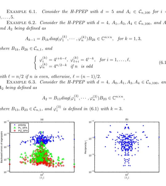
Example 6.1. Consider the H-PPEP with d = 5 and Ai ∈ Cn,100 for i = 0, . . . , 5.
Example 6.2. Consider the H-PPEP with d = 4, A1, A3, A4 ∈ Cn,100, and A0
and A2 being defined as
Ak−1= B1kdiag(ϕ(k)1 , · · · , ϕ(k)n )B2k∈ Cn×n, for k = 1, 3,
where B1k, B2k∈ Cn,1, and (
ϕ(k)i = 4i+k−`, ϕ(k)
`+i= 4i−k, for i = 1, . . . , `,
ϕ(k)n = 4n/2−k if n is odd
(6.1)
with ` = n/2 if n is even, otherwise, ` = (n − 1)/2.
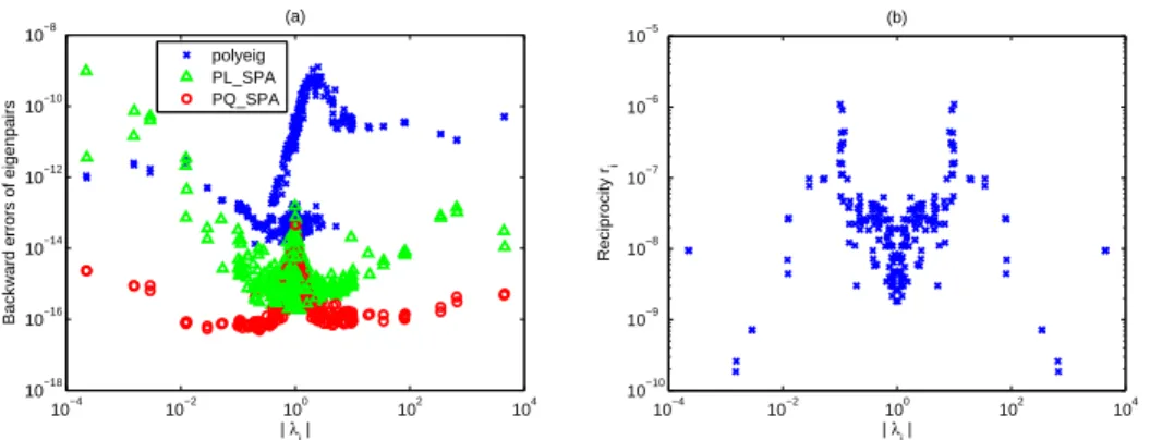
Example 6.3. Consider the H-PPEP with d = 4, A0, A1, A3, A4 ∈ Cn,100, and
A2 being defined as
A2= B13diag(ϕ(3)1 , · · · , ϕ(3)n )B23∈ Cn×n,
where B13, B23∈ Cn,1, and ϕ(3)i is defined in (6.1) with k = 3.
100 10−16 10−15 10−14 10−13 10−12 | λi |
Backward errors of eigenpairs
(a) polyeig PL_SPA PQ_SPA 100 10−15 10−14 10−13 10−12 | λi | Reciprocity r i (b)
Fig. 6.1. Backward errors of eigenpairs and the associated reciprocity for Example 6.1.
10−4 10−2 100 102 104 10−15
10−10 10−5
| λi |
Backward errors of eigenpairs
(a) polyeig PL_SPA PQ_SPA 10−4 10−2 100 102 104 10−8 10−6 10−4 10−2 100 102 | λi | Reciprocity r i (b)
Fig. 6.2. Backward errors of eigenpairs and the associated reciprocity for Example 6.2 with larger kA0k and kA2k.
10−4 10−2 100 102 104 10−18 10−16 10−14 10−12 10−10 10−8 | λi |
Backward errors of eigenpairs
(a) polyeig PL_SPA PQ_SPA 10−4 10−2 100 102 104 10−10 10−9 10−8 10−7 10−6 10−5 | λi | Reciprocity r i (b)
Fig. 6.3. Backward errors of eigenpairs and the associated reciprocity for Example 6.3 with larger kA2k.
We present backward errors and reciprocities of eigenpairs computed by the polyeig, PL SPA and PQ SPA for Examples 6.1–6.3 with fixed matrix dimension
n = 30. Numerical results are shown in Figures 6.1–6.3, respectively. We denote the
results computed by polyeig, PL SPA and PQ SPA by “×”, “4” and “o”, respec-tively. For the PL SPA and PQ SPA, all reciprocities of eigenvalues are preserved to machine accuracy, which are ignored in Figures 6.1 (b)–6.3 (b). From Figures 6.1–6.3, we see that most of backward errors of eigenpairs computed by the PQ SPA are better than that computed by the PL SPA, only a few of the eigenpairs are not. Overall, we conclude that applying the P-quadratization and SPA (Algorithm 3.1) to solve PPEPs not only preserves the reciprocal property but also provides higher accuracy than that by PL SPA and polyeig in MATLAB.
7. Conclusions. In this paper, we propose a palindromic quadratization to transform a (?, ε)-palindromic matrix polynomial of even degree with (?, ε) 6= (T, −1) into a (?, ε)-palindromic quadratic pencil, instead of the palindromic linearization to palindromic linear pencil. Then, the structure-preserving algorithm for solving palindromic quadratic eigenvalue problem based on (S + S−1)-transform and Patel’s algorithm can be applied directly to solve it. We also develop a strategy of balancing and scaling for palindromic matrix polynomials and palindromic quadratic pencils to improve the accuracy of the computed eigenpairs. Numerical experiments show that backward errors of approximated eigenpairs for the palindromic polynomial eigen-value problem computed by the PQ SPA are better than that by the PL SPA and by “polyeig” in MATLAB. Moreover, the computational cost for PQ SPA is clearly much cheaper than that for PL SPA.
Acknowledgments. The authors are grateful to Professor Tisseur and anony-mous referees for many valuable comments and helpful suggestions. This work is partially supported by the National Science Council and the National Center for The-oretical Sciences in Taiwan.
REFERENCES
[1] R. Byers, D. S. Mackey, V. Mehrmann, and H. Xu. Symplectic, BVD, and palindromic ap-proaches to discrete-time control problems. Technical report, Preprint 14-2008, Institute of Mathematics, Technische Universit¨at Berlin, 2008.
[2] E. K.-W. Chu, T.-M. Huang, and W.-W. Lin. Structured doubling algorithms for solving g-palindromic quadratic eigenvalue problems. Technical report, NCTS Preprints in Math-ematics 2008-4-003, National Tsing Hua University, Hsinchu, Taiwan, 2008.
[3] E. K.-W. Chu, T.-M. Hwang, W.-W. Lin, and C.-T. Wu. Vibration of fast trains, palin-dromic eigenvalue problems and structure-preserving doubling algorithms. J. Comput. Appl. Math., 219:237–252, 2008.
[4] N. J. Higham, F. Tisseur, and P. M. Van Dooren. Detecting a definite hermitian pair and a hyperbolic or elliptic quadratic eigenvalue problem, and associated nearness problems. Linear Algebra Appl., 351–352:455–474, 2002.
[5] A. Hilliges. Numerische L¨osung von quadratischen eigenwertproblemen mit Anwendungen in der Schiendynamik. Master’s thesis, Technical University Berlin, Germany, July 2004. [6] A Hilliges, C. Mehl, and V. Mehrmann. On the solution of palindramic eigenvalue problems.
In Proceedings 4th European Congress on Computational Methods in Applied Sciences and Engineering (ECCOMAS), Jyv¨askyl¨a, Finland, 2004.
[7] T.-M. Huang, W.-W. Lin, and J. Qian. Structure-preserving algorithms for palindromic quadratic eigenvalue problems arising from vibration on fast trains. SIAM J. Matrix Anal. Appl., 30:1566–1592, 2009.
[8] C.F. Ipsen. Accurate eigenvalues for fast trains. SIAM News, 37, 2004.
[9] R.-L. Li, W.-W. Lin, and C.-S. Wang. Structured backward error for palindromic polynomial eigenvalue problems. Technical report, NCTS Preprints in Mathematics, National Tsing Hua University, Hsinchu, Taiwan, 2008-7-002, 2008.
[10] W.-W. Lin. A new method for computing the closed-loop eigenvalues of a discrete-time algebraic Riccatic equation. Linear Algebra Appl., 96:157–180, 1987.
[11] D. S. Mackey, N. Mackey, C. Mehl, and V. Mehrmann. Numerical methods for palindromic eigenvalue problems: Computing the anti-triangular Schur form. Numer. Linear Algebra Appl., 16:63–86, 2009.
[12] D.S. Mackey, N. Mackey, C. Mehl, and V. Mehrmann. Structured polynomial eigenvalue prob-lems: Good vibrations from good linearizations. SIAM J. Matrix Anal. Appl., 28:1029– 1051, 2006.
[13] D.S. Mackey, N. Mackey, C. Mehl, and V. Mehrmann. Vector spaces of linearizations for matrix polynomials. SIAM J. Matrix Anal. Appl., 28:971–1004, 2006.
[14] R. V. Patel. On computing the eigenvalues of a symplectic pencil. Linear Algebra Appl., 188:591–611, 1993.
[15] C. Schr¨oder. SKURV: a Matlab toolbox for the skew URV decomposition of a matrix triple. http://www.math.tu-berlin.de/∼schroed/Software/skurv.
[16] C. Schr¨oder. A QR-like algorithm for the palindromic eigenvalue problem. Technical report, Preprint 388, TU Berlin, Matheon, Germany, 2007.
[17] C. Schr¨oder. URV decomposition based structured methods for palindromic and even eigenvalue problems. Technical report, Preprint 375, TU Berlin, MATHEON, Germany, 2007. [18] F. Tisseur. Backward error and condition of polynomial eigenvalue problems. Linear Algebra
Appl., 309:339–361, 2000.
[19] F. Tisseur and K. Meerbergen. A survey of the quadratic eigenvalue problem. SIAM Rev., 43:234–286, 2001.
[20] H. Xu. On equivalence of pencils from discrete-time and continuous-time control. Linear Algebra Appl., 414:97–124, 2006.
[21] S. Zaglmayr. Eigenvalue problems in saw-filter simulations. Diplomarbeit, Institute of Compu-tational Mathematics, Johannes Kepler University Linz, Linz, Austria, 2002.