Paper submitted for the 18th International Input-Output Conference
Stability of I-O technical coefficients by capacity utilization: A case study of the
hotel sector in Taiwan
Dr. Ya-Yen Sun
Assistant Professor, Department of Kinesiology, Health and Leisure Studies (DKHL) National University of Kaohsiung
Tel: 886-7-591-9217 ; Fax: 886-7-591-9264
ABSTRACT
An increasing number of economic impact studies are performed to address special tourism demand conditions such as hosting mega event/ festival or faced with extreme weather, disease outbreaks or terrorist activities. Commonality of these scenarios is that it involves short-term or irregular large-scale demand fluctuation from the baseline point. The adjustment of the I-O coefficient to reflect the cost structure under different demand level is deemed as more critical for the Input-Output analysis. The purpose of this research therefore is to investigate the stability of cost structure by capacity utilization in the tourism industry, using the accommodation sector in Taiwan as an example. Panel data consisting of firm level hotel financial information based on 13 individual cost categories from year 2000 to 2008 is obtained through Taiwan Tourism
Bureau. Panel data analysis is performed to reveal the magnitude and direction of cost structure changes with respect to occupancy rate. For a 10% increase in occupancy from the baseline of 65% occupancy, the intermediate input to sales ratio will decrease from 0.483 to 0.473 while the profit to sales ratio will increase from 0.082 to 0.139, and the employee benefits to sales ratio will decrease from 0.335 to 0.301 for per dollar of final sales. This pattern implies a slight reduced type I sales multipliers and a substantial reduced type II multipliers under a tourism event or festival as the requirement of intermediate input and personal income does not increase proportionally in relation to hotel revenue. On the contrary, a higher type I and type II multipliers can be expected from the standard I-O model during the tourism downtime as a greater
proportion of per dollar revenue is allocated to the inter-industry material, service and employee benefits.
KEYWORD: Capacity utilization, Input-Output Analysis, technical coefficients, accommodation, Taiwan
1. Introduction
The short-term irregular or unexpected demand fluctuation is a special characteristic of the tourism activity. Large-scale demand changes, either positive or negative, are generally resulted from hosting mega event or festival or facing with extreme natural disasters, disease outbreaks or terrorist activities for the destination. While these irregular circumstances become more regular for the tourism industry around the global, an increasing attention is placed on the economic impact analysis to address the large magnitude economy-wide influences. For the one-time demand hike, such as Olympic Games or FIFA World Cup, predicted economic benefits to the region is used by the politicians and proponents to fight for the right to host the game (Lee & Taylor, 2005; Price Water House Coopers, 2005; Toohey & Veal, 2007). For large scale tourism crisis, such as SARS, 911 attack or foot-mouth disease, estimation of economic loss to the business industry, income and job reduction to the region are used to design the recovering policies (Adam Blake & Sinclair, 2003; A Blake, Sinclair, & Sugiyarto, 2003; Siu & Wong, 2004; Yang & Chen, 2009). The economic impacts on intakes or losses to the region are the center focus for all tourism stakeholders when visitor consumption is above or below the average intake in a large magnitude.
Input-Output analysis (I-O) is the frequently adopted method to address the economy-wide impacts by looking at direct, indirect and induced effects of tourism applications. Input-Output analysis computes tourism economic impacts by first converting the final demand changes (e.g., visitor spending) into direct effects in terms of jobs, personal income, tax and value added using economic ratios pertained to the regional economy. Secondary effects are then computed by multiplying the direct effects with the regional multipliers, which are resulted from the inter-industry dependences. Based on the classical I-O assumption, the I-O technical
coefficients, value added component, and the jobs to sales ratio are remained unchanged for the evaluation period, implying constant returns to scale (CRTS) and a linear relationship between final demand changes and total output (Briassoulis, 1991; Miller & Blair, 2009).
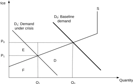
Consider Figure 1 which depicts the demand and supply for consumption goods in a region where short-run supply is fixed and a maximum supply quantity is given as the bottleneck. Two demand curves represent the year-round baseline (D0) and the strong demand condition
under special event or festivals (D1), respectively. Under the baseline scenario, visitor spending
sales or visitor spending equates to area of A, B and C where additional output is increased by (Q1-Q0) and price rising by (P1-P0). Based on standard I-O assumptions, the price factor is
assumed unchanged and constant returns to scale are applied. The model works as if, first, demand expansion only lead to quantity increase, (Q1-Q0) and the additional sales of area B.
Area C does not exist as price would remain constant. Secondly, one set of the production function is assumed in the I-O analysis, as depicted by the I-O technical coefficients, which is applied to final demand change on area A and B.
The reality of business operation, however, introduces the inflation factor in response to sharp demand increase during a short period of time, and may follow changing returns to scale in operation (Chen & Soo, 2007; Lin & Liu, 2000; Perez-Rodrıguez & Acosta-Gonzalez, 2007). Therefore, two sources of errors are introduced in the operation of standard IO model for
evaluating short-term tourism events. First, additional sales volume due to price changes under a higher demand (area C) may require no intermediate input for this proportion of sales as it merely reflects price growth. Price inflation leads to the hypothesis that area C is the major source of overestimation as it will not contribute to the indirect effect, nor will it incur much impact on the introduced effect, depending on the marginal propensity of personal income to sales. Instead, most of the area C should be converted to the business profit. Secondly, under the notion of changing returns to scale with regard to additional sold quantity, area B will not require the same proportion of intermediate inputs as the baseline condition has implied, due to 1) more efficient usages of inputs and labor per sold unit, b) a higher price discount on service and products due to balk purchasing, or 3) possible substitution between input and labors. These
three factors combine leads to a different scale of indirect effect and induced effect in an I-O framework.
Figure 2 on the contrary depicts the demand condition under an abrupt human- or environment-introduced tourism crisis. Sales of the tourism services, under the baseline
condition, are area D, E, and F. Given a tourism crisis with a weak visitor demand, sales quantity is hypothesized to reduce to Q1 while price is decreased to P1. Total sales reduction from the
quantity perspective is measured by area D while sales reduction associated with price is in area E. Based on the standard I-O assumption, sales reduction is only captured by area D as the price factor is not taken into consideration in the model. In addition, based on the operation of constant returns to scale, the model assume input requirement, labor usages, personal income and business profit would reduced in a linear pattern by a ratio of .
S D1: Demand under crisis D0: Baseline demand Quantity Price Q1 Q0 P0 P1 F D E
To reflect the real world operation, the accuracy of impact estimates associated with a tourism crisis, depending on the final demand changes that are fed into the model, and the extent of changing returns to scale that each industry operates. To reflect the first parameter, final demand changes should consider area D only. In other words, if final demand change is
computed as the difference between before-crisis sales (D, E and F) and after-crisis sales (F), it will yield an estimate that is equal to the sum of area D and E taking into account the price adjusted factor. The reduced sales of area E may bear no negative influences on the input
material or staff numbers, and subsequently lead to an overstated job loss or sales reduction from the suppliers. Besides the price factor, the nature of changing return to sales in a short run should not be overlooked as well. The cost structure for a business to operate under a dramatic low
demand condition, in reality, may exhibit a higher ratio of operating cost on intermediate inputs and labors usages while maintaining a relative low business profit on area F.
From this perspective, to accurately portrait the economic impacts for a short-term demand fluctuation therefore rests on the resemblances between a long-run IO technical
coefficients and a short-run production function of the business sectors (Porter & Fletcher, 2008). While most I-O tables are relied on year-long large scale business surveys to compile and may take few years to update, the appropriateness of using the long-run I-O model to study short-term events depends on 1) the price modification of tourism consumption goods and intermediate inputs, and 2) changing returns to scale in business operation. How much is the scale of errors contributed by the individual factor is the focus of empirical studies. Case studies are required to answer following questions as
1. How does business allocate the price-inflated sales (area C) or price deflated sales (area E) to the production function? Will the sales of area C (area E) is attributed to the value added component, mainly to the business profit (losses) or will they incur (reduce) additional inputs in a direct proportion?
2. What is the elasticity between quantity change and price adjustment in response to demand fluctuation? In evaluating the tourism events, what is the ratio between price-lead sales (area C) versus quantity-price-lead sales (area B) for a positive demand hike, or vice versa?
To answer the above questions, capacity utilization is adapted as the key factor to link the demand fluctuation and the stability of I-O Leontief input coefficients for service industries in the short-run. Due to the special service characteristics of intangibility, perishailibty, and simultaneality, the concept of economies of utilization, which is defined as the percentage change in output by one percent increase in all variable input by holding capital fixed, plays a key role in explaining the cost structures of the service sectors, especially for the accommodation, transportation and amusement parks (Caves & Christensen, 1988; Sun, 2007). Under this
concept, for firms operating under constant returns to utilization (CRTU), the cost structures will remain unchanged regardless of the level of output versus capacity. Adopting constant economic ratios and multipliers reflects an unbiased approach. On the other hand, if service entities operate
with increasing returns to utilization (IRTU) or decreasing returns to scale (DRTU), cost structures are subject to changes based on different capacity utilization levels.
The purpose of this paper is to contribute to a better understanding of the firm level cost structure in relation to capacity utilization. The international tourist hotel in Taiwan is selected as the case study by analyzing their expense ratio on 13 different categories in operation.
Relationship between capacity utilization and value added, proportion of personal income, and the dynamics between intermediate input and total sales will be looked into respectively. The main reason for raising the importance on this issue is an increasing number of tourism applications are involved with large scale short-term demand fluctuation. Combined with an increasing tendency for the local tourism agencies to adopt events or festivals as a competitive strategy in position their tourism production (Getz, 2005) and global climate change with increasing probability of extreme weathers, short-term or unexpected demand fluctuation is unavoidable. Our understanding on the firm-level cost adjustment under different capacity
utilization however is not well documented as the financial information on the business operation is confidential and difficult to obtain. The international tourist hotels in Taiwan, required by law, have to submit their financial data to the Taiwan Tourism Bureau every year (Taiwan Tourism Bureau, 2008), providing us an excellent opportunity to evaluate the cost adjustment pattern from an Input-Output framework.
2. Method
Data
A panel data set consisting of yearly Taiwan tourist hotel revenue, cost and operational data from 2000 to 2008 is used for the analysis (Taiwan Tourism Bureau, 2001-2009). Tourist hotels are five-star equivalent with high quality service and relative high prices. Hotel revenue information on rooms, food and beverage, and other income sources are reported along with average room price, yearly occupancy rate and total employee numbers. Hotel operational expenses on 10 categories are reported, including food, laundry, maintenance, utility, insurance, rent, promotion, employee benefits, depreciation and others. A total of 514 cases of yearly operational data from 67 international tourist hotels over the 9-year period is recorded. The data set is examined first for data consistency and accuracy. Cases with incomplete information
across the 9-year period are deleted because they represent entities that have ceased to operate or entered the market less than 9 years. Business that operates under closure crisis or newly open may exhibit different cost structure than those with stable operation in the industry. Since hotels that have constant operation over year 2000 to 2008 accounted for more than 80% of total room capacity and total employees among international tourist hotels, their operational characteristics are deemed representative to the industry average. Therefore, cases that have exited or entered market after year 2000 are excluded and the dataset keeps 414 cases, consisting of 46 hotels. The dataset is maintained with complete cases for both a cross-sectional and a time series dimensions.
To understand how hotels adjust their cost structure in response to capacity utilization within an I-O framework, the firm-level hotel operating costs are divided by its yearly revenue to measure the proportion of dollar input by different cost categories for delivering one dollar of final sales. Therefore, dependent variables, in this study, are
1. the individual cost to sales ratio for the hotel sector: these ratios are computed as costs of food, laundry, maintenance, utility, insurance, rent, promotion, other items, employee salary, and depreciation by total hotel revenue, respectively (Eq.1).
2. profit to sales ratio: firm-level business profit ratio is computed as the yearly revenue minus costs, then divided by revenue.
3. intermediate input to sales ratio: cost of the intermediate inputs summed together to measure the proportion of expenses paid to other sectors, which will result the indirect effects across the economy (Eq.2). On the contrary, employee benefits, business profit, and depreciation in relation to total sales depict the primary input component in the production function (Eq.3).
4. average room price: this ratio is also included as the dependent variable to understand the sensitivity of price adjustment in the accommodation sector.
Independent variable, capacity utilization (CU), is defined as the ratio of actual used (consumed) products to total available products (Berndt & Morrison, 1981). For the
accommodation sector, the occupancy rate (OR) is used as an indicator of capacity utilization (Borooah, 1999), which is computed as the number of occupied rooms to total available rooms (Eq. 3).
nue other reve price * ooms occupied r price * input physical revenue hotel categoy i for the cost ) (CS ratio sales cost to The i i i + = = (1) i: food, laundry, maintenance, utility, insurance, rent, promotion, other items, employee benefits (personal income), and depreciation
revenue hotel CS = cost ratio input to te Intermedia 8 1 i i
∑
= (2)i: food, laundry, maintenance, utility, insurance, rent, promotion, other items
revenue hotel CS = cost ratio input to Primary 3 1 i j
∑
= (3)j: employee benefits, business profit and deprecation
rate occupancy in year t j hotel the of capacity room total in year t j hotel the of ooms occupied r capacity total (services) sold units ) (CU rate tilization Capacity u jt = = = (4)
Economies of utilization is hypothesized for the accommodation sector so that the individual cost and the income to sales ratio would be decreasing when facing with a high occupancy rate. The profit to sales ratio and room price, on the other hand, would be positively related to capacity utilization. As one more room is sold, a higher room price and a profit ratio per room is expected, vice versa. Hypotheses are specified below.
Hypothesis 1: The individual cost to hotel revenue ratio (CS) will be a function of the occupancy rate (OR). A total of 11 equations are specified, whose dependent variables are food cost to sales ratio, maintenance cost to sales ratio, laundry cost to sales ratio, utility cost to sales ratio, insurance cost to sales ratio, rent cost to sales ratio, promotion cost to sales ratio, other items to sales ratio, employee benefits (personal income) to sales ratio, depreciation to sales ratio, and intermediate input to sales ratio. Although a
two-sided hypothesis is applied to examine the relationship between the cost ratio and occupancy rate, coefficients (β’s) are expected to be negative as the economies of utilization is assumed.
E(CSi|OR) = αi + βi*OR (5)
H0: βi = 0
HA: βi ≠ 0
Hypothesis 2: The profit to sales ratio (PS), the value added to sales ratio (VAS), and the average room price will be a function of occupancy rate (OR). A two-sided hypothesis is applied. Coefficients (β's) are expected to be positive as the value added component shall increase with a higher use of occupancy or vice versa.
E(PS|OR) = αj + βj*OR (6)
E(VAS|OR) = αk + βk*OR (7)
E(price |OR) = αl + βl*OR (8)
H0: βj = 0 ; βk = 0 ; βl = 0
HA: βj ≠ 0 ; βk ≠ 0 ; βl ≠ 0
Analysis
Panel data analysis is used to examine firm-specific effects, time effects or both among dependent and independent variables using the Stata software. For each hypothesis, model specification and assumptions are tested first. A linear model is tested using Wald test and Box-Cox method, which compares the linear, log-linear and one general nonlinear model format. Ramsey's RESET test is used to evaluate whether important variables are omitted in the function. Last, Breusch-Pagan / Cook-Weisberg test is applied after controlling for the hotel dummy variables in the regression model for detecting the presence of heteroskedasticity in the error terms.
Panel data models examine the fixed-effect (FE) and the random-effect (RE) of entity (hotel) and/or time. The difference among FE and RE depends on their treatment of group (or time) effects. The FE model assumes group differences in intercepts, and same slopes and
constant variance across entities (Park, 2009; Wooldridge, 2009). The random-effects model, on the other hand, estimates variance components for groups (or times) and assumes the same intercept and slopes.
In this paper, the FE model estimates coefficients using the within method by running OLS in the Stata (Eq.9) (Stata Press, 2009).
x x x (9)
w eh re
,
∑ = / ∑ ∑ /
∑= / , ∑ ∑ /
is the unit specific residual
is the idiosyncratic error ~ IID (0, )
The FE model is preferred over the RE model because first its assumption does not require the independence among group-effect error term and regressors, and secondly, influences from the time-invariant variables, such as hotel location, chain of operation, room capacity can be isolated by the time-demeaning process. Last and the most important reason is that the formula addresses the relationship between the adjustment of the cost ratios and occupancy rates, establishing the relationship between the movement of cost ratios (∆yi) given one percent increase in occupancy
(∆xi). If the cost ratio is relatively constant in relation to demand level, as the I-O model has
assumed, the adjustment of utility ratio (x1-x2) would be close to zero when the occupancy
increases from 40% to 70% occupancy, for example. Under this scenario, the result implies the utility cost and hotel revenue increase in a direct proportion, instead of incurring a fixed amount of utility when demand fluctuates.
A robust Huber-White Sandwich estimator is adopted when heteroskedasticity or within-panel serial correlation in the idiosyncratic error are observed. Dummy variables representing hotel entities are entered in the model to account for unspecified time-varying factors for the individual hotels, such as short-term regional development or adjustment of managerial style. Inclusion of these dummy variables would increase R-squared value but will not influence the
estimation of independent variables that are specified in our hypothesis (Wooldridge, 2009). One-way fixed effect on hotel, one-way fixed effect on year, and two-way fixed effect are examined using F-test, respectively.
The random-effects model is specified as following:
x (10)
Its assumption is that the error of random effect ( is i.i.d., independent from other regressors, and the idiosyncratic error ( is also i.i.d. in the function. If the assumptions are not violated, the RE model produces more efficient results. This strong assumption however is difficult to evaluate in the applied social science and therefore the FE model is generally preferred (Halaby, 2004). The RE model however is not exclusively ruled out in this study but is selected using two criteria. First, the Hausman robust specification test1 is applied to examine whether the
individual effects are uncorrelated with other regressors in the model. If the test fails to reject the RE model, random-effect coefficients and fixed-effect coefficients are compared manually. If both sets of coefficients are similar, do not change signs, and their p-values are not substantial different to reject/accept the alternative hypothesis, the fixed-effect estimator is preferred. Robust estimators and two-way random effects are applied when necessary.
3. Results
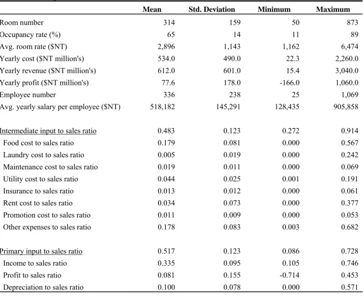
Descriptive information. Among the 46 international tourist hotels in Taiwan, the hotel
capacity ranges between 50 rooms to 873 rooms per entity with an average of 314 rooms. The occupancy rate fluctuates between 11% and 89% for all tourist hotels, with an average room rate of NT$29002. A total of 15,456 employees are employed by the tourist hotel entities at these 46 hotels, providing employee benefits of NT$ 0.52 million per person per year. During the
operation of year 2000 to 2008, expenses for the intermediate inputs exhaust 48% of total hotel revenue. Among all categories, “other expenses” accounted for 17.8%, followed by food cost,
1 See Baltagi (2008, pp. 72-78) for a summary of tests for fixed versus random effects. See Cameron & Trivedi
(2009, pp. 261-262) for STATA syntax.
2 Currency denoted in the paper is New Taiwan Dollars ($NT). One US dollar is approximately equal to NT$32 in
17.9% and utility cost, 4.4%. Primary input, on the other hand, is mainly allocated to the
employee benefits (33.5%) and depreciation (10.0%). The business profit, on average, is around 8.1% of total revenue at the occupancy of 65% during 2000 and 2008.
Table 1. Descriptive statistics of tourist hotels in Taiwan, 2000-2008
Mean Std. Deviation Minimum Maximum
Room number 314 159 50 873
Occupancy rate (%) 65 14 11 89
Avg. room rate ($NT) 2,896 1,143 1,162 6,474
Yearly cost ($NT million's) 534.0 490.0 22.3 2,260.0 Yearly revenue ($NT million's) 612.0 601.0 15.4 3,040.0 Yearly profit ($NT million's) 77.6 178.0 -166.0 1,060.0
Employee number 336 238 25 1,069
Avg. yearly salary per employee ($NT) 518,182 145,291 128,435 905,858
Intermediate input to sales ratio 0.483 0.123 0.272 0.914 Food cost to sales ratio 0.179 0.081 0.000 0.567
Laundry cost to sales ratio 0.005 0.019 0.000 0.242 Maintenance cost to sales ratio 0.019 0.011 0.000 0.069 Utility cost to sales ratio 0.044 0.025 0.001 0.191 Insurance to sales ratio 0.013 0.012 0.000 0.061 Rent cost to sales ratio 0.034 0.073 0.000 0.377 Promotion cost to sales ratio 0.011 0.009 0.000 0.053 Other expenses to sales ratio 0.178 0.083 0.003 0.682
Primary input to sales ratio 0.517 0.123 0.086 0.728
Income to sales ratio 0.335 0.095 0.105 0.746 Profit to sales ratio 0.081 0.155 -0.714 0.453 Depreciation to sales ratio 0.100 0.078 0.000 0.571
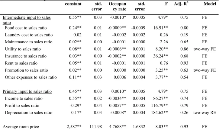
Regression results. Eleven out of the fourteen equations are estimated using the one-way
fixed effect model on hotel with a Huber-White Sandwich estimator due to the presence of heteroskedasticity in the error terms. Utility cost and promotion cost are estimated with the two-way fixed effect model by considering both the entity and time effect simultaneously. Based on the data, hotel investment for promotion and marketing campaign was decreasing over the years as well as the promotion expenses to sales ratio, which is decreased from 1.48% of total revenue in 2000 to 1.02% in 2008. In contrast, a trend of steady increasing utility to sales ratio (water,
electricity and gas) by years was observed for the hotel operation, ranging from 3.36% in year 2000 to 3.87% in 2008. For both cases, using a two-way fixed effect model controls the hotel and time effects so that the influence of occupancy rate on the dependent variables can be identified.
For the intermediate input to sales ratio, for every 1% increase in occupancy rate, the ratio is expected to decrease 0.001, ceteris paribus (Table 2). This implies the allocation of hotel revenue in purchasing operation goods and service from other industries is reduced in a rate of 2.1%, signaling a reduced type I sales multipliers for every dollar of final changes (table 3). Among the expenses categories, cost ratios on food, utility, and insurance are expected to decrease given a higher occupancy. On the contrary, the laundry ratio, maintenance ratio, rent ratio, promotion ratio and other expenses ratio are not influenced by the occupancy rate at the 95% significant level. This implies a relatively fixed ratio of hotel revenue is allocated to these 5 categories disregarding the adjustment of occupancy.
Table 2. Results of panel data analysis
constant std. error Occupan cy rate std. error F Adj. R2 Model
Intermediate input to sales
ratio 0.55** 0.03 -0.0010* 0.0005 4.79* 0.75 FE Food cost to sales ratio 0.24** 0.01 -0.0009** -0.0009 16.91** 0.80 FE Laundry cost to sales ratio 0.02 0.01 -0.0002 0.0002 0.26 0.19 FE Maintenance to sales ratio 0.02** 0.00 -0.0001 0.0000 2.26 0.65 FE Utility to sales ratio 0.08** 0.01 -0.0006** 0.0001 8.20** 0.86 two-way FE Insurance to sales ratio 0.03** 0.00 -0.0002** 0.0000 36.24** 0.68 FE Rent to sales ratio 0.05** 0.01 -0.0001 0.0001 0.76 0.93 FE Promotion to sales ratio 0.02** 0.00 0.0000 0.0000 3.25** 0.63 two-way FE Other expenses to sales ratio 0.11** 0.03 0.0006 0.0004 3.77** 0.54 FE Primary input to sales ratio 0.45** 0.03 0.0010* 0.0005 4.79* 0.75 FE Income to sales ratio 0.55** 0.02 -0.0034** 0.0004 86.27** 0.74 FE Profit to sales ratio -0.29* 0.04 0.0057** 0.0005 116.79** 0.79 FE Depreciation to sales ratio 0.17* 0.03 -0.0008* 0.0004 184.62** 0.26 two-way RE Average room price 2,587** 111.98 4.7688** 1.6832 8.03** 0.93 FE
Note: The dependent variable is shown in the row heading, and the explanatory variables are shown in the column heading. **Significant at the 99% level; *significant at the 95% level.
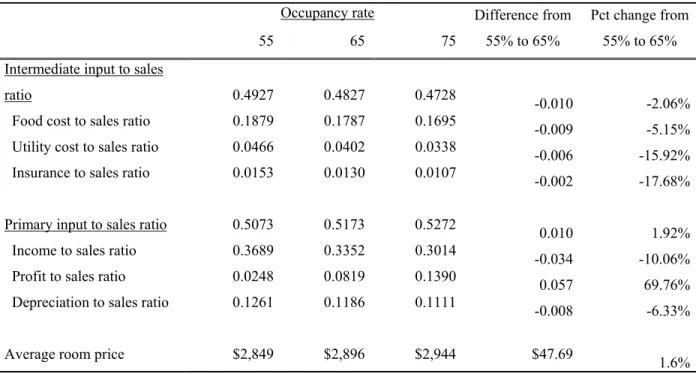
For the primary input to sales ratio, for every 10% increase in occupancy rate, the ratio is expected to increase 0.01 or 1.9%, ceteris paribus, parallel to the ratio of the intermediate input (Table 2). When occupancy increases from the baseline point of 65% to 75%, the profit ratio is expected to increase from 8.19% to 13.90% (+5.71%) while the employee benefits ratio reduced from 33.52% to 30.14% (-3.38%), and the depreciation ratio decreased from 12.61% to 11.86% (-0.75%). Based on the operation of the hotel industry, the addition of hotel revenue at a higher occupancy is attributed to the business profit in a greater proportion while the overall employee benefit to sales ratio is reduced. In contrast, when the business is operating under the low demand and low occupancy, for example, 55%, the reduced sales is absorbed by the business itself as a shrinking profit without decreasing the employee benefits in a direct proportion. If not considering the tax factor, the break-even point for the tourist tourists, on average, is at the occupancy of 50.7%. Below this point, an operation deficit is expected. Room price is also fluctuated along with occupancy. Given a 10% occupancy increase, additional $47.7 dollars or 1.6% price hike per room is expected to be charged.
Table 3 Predicted ratios by occupancy rate
Occupancy rate Difference from 55% to 65%
Pct change from 55% to 65% 55 65 75
Intermediate input to sales
ratio 0.4927 0.4827 0.4728 -0.010 -2.06%
Food cost to sales ratio 0.1879 0.1787 0.1695 -0.009 -5.15% Utility cost to sales ratio 0.0466 0.0402 0.0338 -0.006 -15.92% Insurance to sales ratio 0.0153 0.0130 0.0107 -0.002 -17.68% Primary input to sales ratio 0.5073 0.5173 0.5272 0.010 1.92% Income to sales ratio 0.3689 0.3352 0.3014 -0.034 -10.06% Profit to sales ratio 0.0248 0.0819 0.1390 0.057 69.76% Depreciation to sales ratio 0.1261 0.1186 0.1111 -0.008 -6.33% Average room price $2,849 $2,896 $2,944 $47.69 1.6%
4. Discussion
Using the year-long average cost structure to perform the short-term ex-ante or ex-post economic impact analysis inherit estimation errors if business are operating under changing returns to utilization and the price factor is taken into consideration. Using tourist hotels in Taiwan as an example, for every 10% increase in occupancy, the intermediate input to sales ratio will decrease by 1.0% while the profit to sales ratio will increase by 5.7% and the employee benefits to sales ratio will decrease by 3.4% or vice versa. Among all intermediate inputs to the hotel operation, food to sales ratio, utility to sales ratio, and insurance to sales ratio fluctuate along with occupancy rate at 99% significant level while laundry, maintenance, rent, promotion and other expenses to sales ratio do not. We further divide the independent variables based on the regression results into three groups:
1. Coefficient (β) is not significant at the 95% level. Cost categories include laundry, maintenance, rent, promotion and other expenses ratio.
2. Coefficient (β) is significant at the 95% level but the coefficient is relatively small. For every 10% of occupancy changes, the coefficient will fluctuate less than 0.01 from the baseline point. Cost categories include food, utility, insurance and depreciation. 3. Coefficient (β) is significant at the 95% level but the coefficient is relatively large. For
every 10% of occupancy changes, the coefficient will fluctuate more than 0.01. Cost categories include employee income and business profit.
The level of estimation error in a standard I-O model can be classified based on these three groups. Group 1 will bear less estimation error as this ratio will not fluctuate from the perspective of occupancy rates, implying a relatively stable input to sales ratio. Impacts of the cost items under the group 2 will tend to be overestimated for a higher occupancy or vice versa due to economies of utilization, but the level of estimation error is negligible. Compared to the first two groups, a greater attention should be placed on the computation of the group 3 variables, personal income and business profits. These two coefficients are strongly complemented.
Overestimation of business profits is mainly at the expenses of employee benefits under a low occupancy scenario.
Results from this case study imply a reduced type I sales multipliers and type II multipliers from the baseline point under a tourism event or festival as the requirement of intermediate input and personal income does not increase proportionally in relation to additional hotel revenue. On the contrary, a larger type I and type II multipliers can be expected during the tourism downtime as a greater proportion of per dollar revenue is allocated to the inter-industry material, service and employee benefits. This pattern can be explained by the short-term nature of tourism demand fluctuation, which prevents the business entity to implement immediate cost adjustment policies. Strategies such as capacity expansion, technical adoption, employee recruitment or displacement are difficult, inefficient and risky in the short-run as these final demand changes will not last permanently.
The merit of this study is to provide the empirical evidence regarding the adjustment of cost structure from an I-O framework. For practitioners involving with I-O models, the question boils down to whether such an adjustment of the I-O coefficients is worth implementing as every adjustment to the model requires additional effort in data collection and the model building. The issue to tackle the accuracy of economic impact studies has been addressed from two
perspectives in the literature: final demand changes and the economic model. Frechtling (2006), Stynes & White (2006) and Wilton & Nickerson (2006) felt that a greater effort should be made toward improving and implementing a well organized visitor survey for gathering visits and expenditure. From their perspectives, the bias of visitor spending measurement is the possible biggest error during the economic impact estimation process. The advocators of Computable General Equilibrium (CGE) model, on the other hand, are devoted to the model improvement by relaxing most of the standard I-O assumption by taking into account the factor constraints, household consumption, real wages flexibility, price factor, and governmental fiscal policy stance (Dwyer, Forsyth, & Spurr, 2004, 2005, 2006a, 2006b)3. CGE models are generally applied at the national level and their outputs are more conservative and the negative impacts on exports, employment, or tax dollars on other non-tourism sectors or rest of the area can be analyzed.
Currently, while most regional economic impact analysis are still relied on the I-O model, results from this study can be used to suggest priorities in the I-O model adjustment. For
3 See Dwyer, Forsyth, & Spurr (2006b, p. 324) for a good comparison of assumptions using in a standard I-O model
scenarios that involve a large-scale demand fluctuation, the over-(under-) estimation of business profits vs. employee benefits are too large to overlooked. For an increase of 30% in occupancy for the accommodation sector, which is quite common among short-term tourism applications, the business profits will be underestimated by 17% while the employee benefits will be
overestimated by 10% for every dollar of final sales. Such information provides practitioners with a tool to compare the variance range of visits, average spending and the cost structure before additional efforts are invested to address the accuracy of economic impact estimates.
Limitations of this study are first, changes of regional propensity to import cannot be identified in our dataset as input material can be supplied by the domestic or international goods. Secondly the time dimension of our data is based on the annual operation. The monthly or weekly room price or cost adjustment is embedded and averaged out in the dataset. Short-term room price and cost adjustment should be more substantial than what the coefficients have suggested here. The estimation error for the value added component should be more serious when the final demand change is lasted only for a few weeks or months. Lastly, the data is limited to the tourist hotels in Taiwan without considering other tourism sectors, such as
transportation, amusement parks, restaurants or other recreation service providers. In addition to the challenge of data scarcity, the concept of capacity utilization is more difficult to implement in other tourism sectors, making the evaluation of cost adjustment inoperative.
5. Reference
Baltagi, B. H. (2008). Econometric Analysis of Panel Data (4th ed.). Chichester, UK: Wiley. Berndt, E. R., & Morrison, C. J. (1981). Capacity utilization measures: Underlying economic
theory and an alternative approach. The American Economic Review, 71(2), 48-52. Blake, A., & Sinclair, M. T. (2003). Tourism crisis management: US Response to September 11.
Annals of Tourism Research, 30(4), 813-832.
Blake, A., Sinclair, M. T., & Sugiyarto, G. (2003). Quantifying the impact of foot and mouth disease on tourism and the UK economy Tourism Economics, 9(4), 449-465.
Borooah, V. K. (1999). The supply of hotel rooms in Queensland, Australia. Annals of Tourism
Research, 26(4), 985-1003.
Briassoulis, H. (1991). Methodological issues: Tourism input-output analysis. Annals of
Tourism Research, 18(3), 485-495.
Cameron, A. C., & Trivedi, P. K. (2009). Microeconometrics Using Stata. College Station, Texas: Stata Press.
Caves, D. W., & Christensen, L. R. (1988). The importance of economies of scale, capacity utilization, and density in explaining interindustry differences in productivity growth.
Logistics and Transportation Review, 24(1), 3-32.
Chen, C.-F., & Soo, K. T. (2007). Cost structure and productivity growth of the Taiwanese international tourist hotels. Tourism Management, 28(6), 1400-1407.
Dwyer, L., Forsyth, P., & Spurr, R. (2004). Evaluating tourism's economic effects: New and old approaches. Tourism Management, 25(3), 307-317.
Dwyer, L., Forsyth, P., & Spurr, R. (2005). Estimating the impacts of special events on an economy. Journal of Travel Research, 43, 351-359.
Dwyer, L., Forsyth, P., & Spurr, R. (2006a). Assessing the economic impacts of events: A computable general equilibrium approach Journal of Travel Research, 45(1), 59-66. Dwyer, L., Forsyth, P., & Spurr, R. (2006b). Economic evaluation of special events. In L. Dwyer
& P. Forsyth (Eds.), International handbook on the economics of tourism. Glos, UK: Edward Elgar Publishing Limited.
Frechtling, D. C. (2006). An Assessment of Visitor Expenditure Methods and Models. Journal of
Travel Research, 45(1), 26-35. doi: 10.1177/0047287506288877
Getz, D. (2005). Event Management & Event Tourism (2nd ed.): Cognizant Communication Corp.
Halaby, C. N. (2004). Panel Models in Sociological Research: Theory into Practice. Annual
Review of Sociology, 30, 507-544.
Lee, C.-K., & Taylor, T. (2005). Critical reflections on the economic impact assessment of a mega-event: the case of 2002 FIFA World Cup. Tourism Management, 26(4), 595-603. Lin, B.-H., & Liu, H.-H. (2000). A study of economies of scale and economies of scope in
Taiwan international tourist hotels. Asia Pacific Journal of Tourism Research, 5(2), 21 - 28.
Miller, R. E., & Blair, P. D. (2009). Input-output analysis: Foundations and extensions (2nd ed.). Cambridge, UK: Cambridge University Press.
Park, H. M. (2009). Linear Regression Models for Panel Data Using SAS, Stat, Limdep, and SPSS. Working Paper: The University Informaiton Technology Services (UITS) Center for Statistical and Mathematical Computing, Indiana University.
Perez-Rodrıguez, J. V., & Acosta-Gonzalez, E. (2007). Cost efficiency of the lodging industry in the tourist destination of Gran Canaria (Spain). Tourism Management, 28(4), 993-1005. Porter, P. K., & Fletcher, D. (2008). The economic impact of the Olympic Games: Ex ante
predictions and ex poste reality. Journal of Sport Management, 22, 470-486.
Price Water House Coopers. (2005). Olympic Games Impact Study. London: Price Water House Coopers LLP.
Siu, A., & Wong, Y. C. R. (2004). Economic Impact of SARS: The case of Hong Kong. Asian
Economic Papers, 3(1), 62-83. doi: doi:10.1162/1535351041747996
Stata Press. (2009). Stata Longitudinal-Data/Panel-Data Reference Manual: Release 11: Stata Press.
Stynes, D. J., & White, E. M. (2006). Reflections on Measuring Recreation and Travel Spending.
Journal of Travel Research, 45(1), 8-16. doi: 10.1177/0047287506288873
Sun, Y.-Y. (2007). Adjusting Input-Output models for capacity utilization in service industries.
Taiwan Tourism Bureau. (2001-2009). The operating report of international tourist hotels in Taiwan. Taipei, Taiwan: Tourism Bureau, Ministry of Transportation and
Communications, R.O.C.
Taiwan Tourism Bureau. (2008). Regulation for the management of tourist hotel enterprises. Taipei, Taiwan: Tourism Bureau, Ministry of Transportation and Communications, R.O.C.
Toohey, K., & Veal, A. J. (2007). The Olympic Games: A social science perspective (2nd ed.). Oxfordshire, UK: CABI International.
Wilton, J. J., & Nickerson, N. P. (2006). Collecting and Using Visitor Spending Data. Journal of
Travel Research, 45(1), 17-25. doi: 10.1177/0047287506288875
Wooldridge, J. M. (2009). Introductory Econometrics: A Modern Approach (4th ed.). Cincinnati, OH: South-Western.
Yang, H.-Y., & Chen, K.-H. (2009). A general equilibrium analysis of the economic impact of a tourism crisis: A case study of the SARS epidemic in Taiwan. Journal of Policy Research
in Tourism, Leisure and Events, 1(1), 37-60.