The Effect of .99 Price Endings on Consumer
Demand: An Example of Confounding Factors
Surviving in Field Experiments
Antonio Filippin
*Dipartimento di Economia, Management e Metodi Quantitativi, Università degli Studi di Milano, Italy
The paper investigates the effect of .99 price endings on consumer demand by means of a field experiment. Results tail behind other contributions showing how .99-endings can be ineffective, casting doubts on their widespread use among retailers. When the .99-ending price is removed an increase of sales emerges from descriptive statistics as well as in a multivariate framework in which sales of the treated item are the only dependent variable. However, such a counterintuitive effect does not survive in a differences-in-differences model in which the daily sales of all the relevant substitutes are jointly analyzed. There is no evidence of any common shock during the treatment. In contrast, a different price-elasticity of demand drives the relative increase of sales of the treated item when prices of the substitutes are on average higher. Once the different reactions to price changes are taken into account, the treated item does not display significantly higher sales as compared to its substitutes when the .99-ending price is removed.
Keywords: price ending, field experiment, pricing JEL classification: C93, D12, L11, M31
*Correspondence to: Dipartimento di Economia, Management e Metodi Quantitativi, Università
degli Studi di Milano, Italy. Email: antonio.filippin@unimi.it. I would like to thank Massimiliano Bratti, three anonymous referees as well as participants at the International ESA Meeting (Rome) for helpful suggestions. The usual disclaimers apply.
1
□
Introduction
The analog (or holistic) model of numerical cognition (Dehaene, 1997; Hinrichs et
al., 1981) suggests that when presented with two multi-digit numbers to be
compared we assess their quantitative meaning by spontaneously mapping them onto an internal mental magnitude scale. Nine-endings favour two very similar numbers to be assigned to different internal magnitudes. Thomas and Morwitz (2005) claim that what makes the nine-endings salient is the left-to-right processing of numerical symbols. Therefore, the effect of a nine-ending is more relevant when it implies a change in the leftmost digit. When using a nine-ending versus a zero-ending implies a change in the leftmost digit (e.g. $2.99 versus $3.00) it is this change, rather than the one cent drop, that affects the magnitude perception.
Byzer and Schindler (2005) find that experimental subjects indeed think they could buy significantly more products priced with 99-endings than products with comparable 00-ending prices. Basu (2006) applies this mechanism to an oligopolistic model à la Bertrand showing that undercutting below .99 becomes less likely, thereby making .99-ending prices both more frequent and more sticky.
This theoretical framework accounts for the widespread use of nine price endings among retailers. Levy et al. (2011) using weekly scanner data as well as Internet data find that nine is the most frequent ending, that the most common price changes are those that keep the price endings at nine, and that nine-ending prices are less likely to change. Some studies report that 30% to 65% of all prices end in the digit nine (Stiving and Winer, 1997; Schindler and Kirby, 1997). Hackl, Kummer, and Winter Ebmer (2010) find a slightly lower percentage (20%) in a large dataset gathered from an Austrian online shopping site that compares prices of several suppliers of microelectronic products. Stiving (2000) shows that nine price endings are less frequent when firms are signaling high quality with high prices. Schindler (2006) documents that a 99-ending is more likely to be associated with low-price cues in newspaper advertising.
Although the use of nine price endings is widespread, the evidence supporting their effectiveness is weaker than one could expect at first glance, starting from the seminal paper by Ginzberg (1936), who reports that customary prices do not
systematically increase sales as compared to rounded prices. Among the contributions that provide evidence supporting the effectiveness of nine-ending prices in increasing consumers demand there are Anderson and Simester (2003), who manipulate prices in mail order catalogues, and Kalyanam and Shively (1998), who find significant spikes of sales at nine-ending prices for stick margarine and canned tuna using scanner data. Hackl, Kummer, and Winter Ebmer (2010) report that .99 is the most clicked among all focal prices even when it is not the cheapest one. In contrast, both Stiving and Winer (1997) using packaged goods like canned tuna and yoghurt, and Schindler and Kibarian (1996) using women’s clothing in a mail order catalogue display inconclusive results. Finally, Georgoff (1972) finds no effect.
A possible explanation for the mixed evidence is that nine-ending prices have an effect, but that such an effect is not uniformly strong because it depends on the characteristics of the good (type, quality, price level, size and direction of the price change, etc.). However, the aforementioned contributions do not allow to identify sufficiently robust and systematic patterns.
Causal relationships about decision making are often tested by means of laboratory experiments that reproduce economic choices in a controlled, aseptic setting where the effects of exogenous treatments on behaviour can be observed. Laboratory experiments, however, are criticized on the grounds of their weak external validity. When feasible a field experiment represents a useful tool of analysis, especially when it allows to observe choices that occur in their natural environment, with agents facing the natural consequences of their actions. Of course, with a field experiment some control gets lost as compared to a lab experiment, but as Harrison and List (2004) point out this caveat is counterbalanced by the advantages connected to observing agents’ behaviour without interfering in any way with their decision process and the environment where it takes place.
This paper aims at investigating the effect of .99-ending prices on consumer demand by means of a field experiment conducted in an Italian supermarket, in which the price of two local brands of mozzarella cheese have been modified in a controlled manner. The choice of mozzarella cheese is due to two main reasons. First, it is purchased quite frequently by many consumers and it cannot be stockpiled because it must be consumed within a few days. This is crucial in order to assume
that the effects of discounts rather frequent in the supermarkets do not have long-lasting effects. This maximizes the importance of current relative prices in explaining consumer demand. Second, it is characterized by a standard quality, so that the choice of purchasing the item cannot rely upon the subjective evaluation of its quality, something that could not be controlled for during the experiment. For instance, fruits and vegetables would perfectly fulfil the first requirement while failing the second. The opposite would happen for storable products.
2
□
Design of the Experiment
The design of the experiment involves two brands of mozzarella cheese that have been evaluated as almost perfect substitutes ex ante, simply called Brand A and Brand B in what follows. Brand A is the treated item because it is the one already characterized by a price equal to €.99 before the experiment. There are two main reasons to include also Brand B as control in the design of the experiment. First, within a brand choice framework sales of the closest substitute are where we expect to observe the strongest flows in or out when a shock, like the treatment of this experiment, hits the price of Brand A. Second and foremost, Brand B constitutes a natural control for every unobservable shock affecting Brand A as well. In other words, choosing an item as similar as possible to Brand A maximizes the likelihood that unobservable shocks are common to both mozzarella cheeses. Suppose in fact that some conditions change in the period covered by the experiment. If it is an observable variable (like the pattern of daily sales in the supermarket, the change of prices of substitutes, etc.) the effect can be easily controlled for in a multivariate regression. However, if the data do not keep track of the change (e.g. a fair of local food), such a determinant would be out of the control of the experimenter and would bias the estimate of the role played by the .99 price ending unless it is somehow accounted for.
Of course, there are many substitutes of Brand A in the store, but it was not possible to manipulate the price of all the items. Hence, the choice has been to change the price of the treated brand and that of the closest substitute only. Brand A and Brand B are both made of cow’s milk, they are equal in terms of weight (100g.) and very similar in terms of price. Both represent old local dairies from the same
Italian region (Liguria), although the goods are now produced in other regions (Brand A in Lombardy and Brand B in Emilia Romagna). The two brands are next to each other in the shelf layout and therefore consumers can compare their prices very easily. According to their experience, the store managers agreed that the items chosen for the experiment were the best substitutes among the mozzarella cheeses. An ex post analysis of historical data also confirms this claim, given that a cross-elasticity of about +2.3 emerges in a multivariate framework when sizeable price discounts of Brand B (at least 10%) are implemented.1
To avoid the introduction of an idiosyncratic shock to Brand A that could confound the results, the experiment imposes the same price change to both brands, although the price variation is almost negligible (about 2%). The prices usually displayed are €.99 for Brand A and €.94 for Brand B.2 For a period of four weeks the two prices have been increased by the same percentage to €1.01 and €.96, respectively (see Table 1). Variations have been implemented without semantic cues suggesting to consumers that the prices have been modified, something that Anderson and Simester (2003) have shown to have an additional effect on sales. Also the shelf display remained the same during the treatment.3
Table 1: Prices of the Two Brands of Mozzarella Cheese
Before 2 May – 4 June Treatment 5 June – 3 July After 4 July –12 Nov Brand A 0.99 1.01 0.99 Brand B 0.94 0.96 0.94
If sales of Brand B were a perfect control for all the unobservable shocks that could hit sales of Brand A in the period of the analysis, removing the .99-ending price would be the only shock affecting Brand A, thereby allowing us to give a causal interpretation of the results.
1The cross-elasticity of Brand B cannot be computed because there are no significant changes in the
price of Brand A in the sample available.
2
The price of Brand B has been discounted twice, the first time before the treatment, the second time afterwards. However, there are at least ten days before and after the treatment in which the price was the usual one (€.94).
3The approval to perform the experiment was subordinate to the minimization of the impact on the
point of sale. This prevented the experimental design from including other treatments, such as items of different value, different price manipulations, etc. that would have made the experiment more informative.
Unfortunately, the loss of control implied by the characteristics of a field experiment imposes to be careful, because even a very accurate design of the experiment is not sufficient to rule out other idiosyncratic shocks. Hence, the pattern of the other substitutes will be analyzed, too.
Excluding the two brands included in the treatment it is possible to distinguish other 49 different types of mozzarella cheese in the store, according to their quality, brand, and size. Twenty-eight can be considered poor substitutes of Brand A and B, because they are very different (made from the milk of buffalo, bio, light, high quality, only for pizza, etc.). Other twenty-one differ in terms of size and/or brand, some are also multipack, but their quality cannot be assumed to be too different and therefore they have to be taken into account because what happens to them can potentially be informative as far the sales of Brand A and B are concerned. Only twelve, however, are explicitly considered when analyzing the results of the experiment because the others either do not display any price variation or are characterized by a negligible amount of sales.
The implication tested by the experiment is that if the use of the .99-ending price is smoothly associated to an increase of sales, we should observe lower sales of Brand A relative to those of Brand B during the experiment when the .99 price ending disappears. In order to exclude that other confounding factors can affect the results, data are also analyzed using a differences in differences (DID) approach, so that only the change in the sales of Brand A relative to all the other brands matters.
3 Results
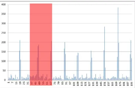
The dataset contains daily prices and sales of 14 types of mozzarella cheese for a period of about six months (193 days). The daily sales of Brand A, the treated mozzarella cheese, display a weird pattern, as shown in Figure 1, where the shadowed area represents the period in which the treatment took place.
Note: The shadowed area corresponds to the treatment
Figure 1: Average Daily Sales of Brand A
Sales are characterized by spikes that happen always during the weekend every two or three weeks, regardless of the prices of Brand A as well as that of the other brands of mozzarella cheese. Such a pattern could be explained for instance by regular purchases by big customers (e.g. restaurants or pizzerias). Unfortunately, for privacy reasons the chain store did not release the microdata collected through their fidelity cards, which could easily shed some light on the matter. Such spikes occur with a regular frequency but they distort the results of the treatment nevertheless.4 A similar pattern does not characterize any of the other brands, thereby constituting an idiosyncratic shock to the treated item for which no specific control is available. Hence, they are removed from the analysis leaving 166 days included in the dataset.
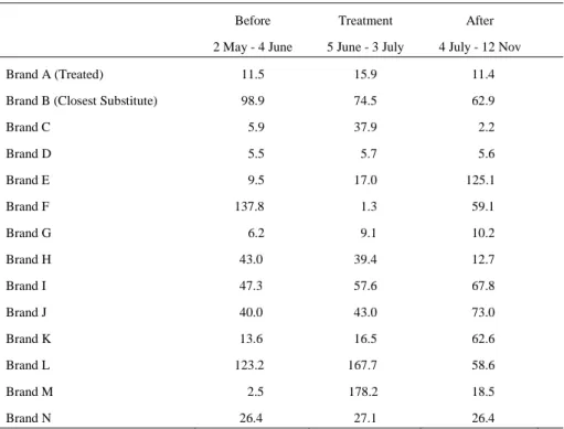
Table 2 reports the average daily sales of all the 14 relevant brands of mozzarella cheese before, during, and after the treatment. It is immediately evident the variance that characterizes some brands, which is driven by discounts.
4Out of nine spikes, two take place during the experiment (35 days), while the other seven occur in
the control period (158 days). Given that the spikes are on average similar in terms of magnitude the different frequency creates an upward bias to the sales during the treatment that needs to be removed. In fact, keeping these outlier observations in the analysis would artificially reverse the findings presented below.
Unfortunately, also the price of Brand B has been discounted twice for a period of two weeks, the first time (by 20%) before and the second time (by 10%) after the treatment.
Table 2: Average Daily Sales of All the Relevant Mozzarella Cheeses
Before Treatment After
2 May - 4 June 5 June - 3 July 4 July - 12 Nov
Brand A (Treated) 11.5 15.9 11.4
Brand B (Closest Substitute) 98.9 74.5 62.9
Brand C 5.9 37.9 2.2 Brand D 5.5 5.7 5.6 Brand E 9.5 17.0 125.1 Brand F 137.8 1.3 59.1 Brand G 6.2 9.1 10.2 Brand H 43.0 39.4 12.7 Brand I 47.3 57.6 67.8 Brand J 40.0 43.0 73.0 Brand K 13.6 16.5 62.6 Brand L 123.2 167.7 58.6 Brand M 2.5 178.2 18.5 Brand N 26.4 27.1 26.4
What emerges at first glance is a counterintuitive increase of sales of Brand A. As already pointed out in the previous section, however, this cannot be immediately attributed to the treatment because other factors may be at work. For this reason I perform a multivariate analysis in which several controls are used in order to control for the observable and possibly also for the unobservable confounding factors. Two different estimation strategies are adopted. The first entails the sales of Brand A as the unique dependent variable. The second is instead a differences-in-differences (DID) approach in which the sales of all the relevant mozzarella cheeses are considered at the same time. The reason to use a DID framework is that ex post Brand B turned out to be not as good a substitute as it seemed ex ante.
3.1 A Multivariate Analysis of the Sales of Brand A
This section specifically analyses the sales pattern of Brand A controlling for some observable shocks and using sales of Brand B as a control for the unobservable ones.
The specification estimated is the following:
YA = γ0 + γ1T + γ2YB + γ3 X + εA,
where:
YA = Daily sales of Brand A,
T = Treatment: dummy variable equal to one when the .99 price is removed, YB = Daily sales of Brand B,
X = Vector of controls (price of all the brands, total sales).
Including the total daily sales of all the 51 types of mozzarella cheese controls for the possibility that sales of Brand A simply follows a general pattern. For instance, suppose that the weather conditions have been better in the month in which the .99 price has been removed, thereby increasing the consumption of all mozzarella cheeses. If this is the case, the observed increase of sales of Brand A would just be spuriously correlated with the treatment. This variable is also a good proxy for the weekly business cycle of the store.
Promotions that concern other mozzarella cheeses can affect sales of Brand A as long as they can be considered as substitutes. There are twelve other items of this type besides Brand B and promotions are quite frequent. Hence, either the daily price of each substitute or a variable that summarizes how many substitutes are on discount day by day are included in two different versions of the estimated model.
As already explained, the possible effect of other shocks, either unobservable or in any case not accounted for by the aforementioned controls can be captured in principle by the daily sales of Brand B, i.e. the closest substitute of the treated mozzarella cheese. By including this variable, any shock that has the same effect on both brands should not interfere with the experiment.
If all these factors are properly accounted for, the dummy variable representing the treatment ( T ) captures the causal effect of removing the .99 price on the average sales pattern of Brand A.
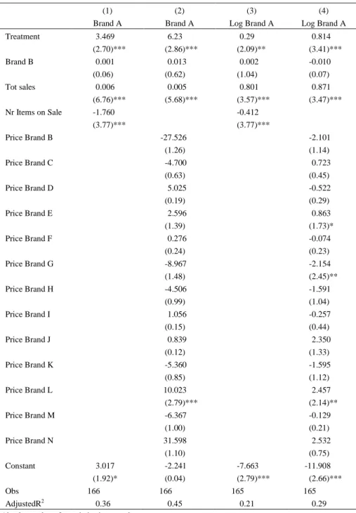
Table 3: Multivariate Analysis of Daily Sales of Brand A
(1) (2) (3) (4)
Brand A Brand A Log Brand A Log Brand A
Treatment 3.469 6.23 0.29 0.814 (2.70)*** (2.86)*** (2.09)** (3.41)*** Brand B 0.001 0.013 0.002 -0.010 (0.06) (0.62) (1.04) (0.07) Tot sales 0.006 0.005 0.801 0.871 (6.76)*** (5.68)*** (3.57)*** (3.47)*** Nr Items on Sale -1.760 -0.412 (3.77)*** (3.77)*** Price Brand B -27.526 -2.101 (1.26) (1.14) Price Brand C -4.700 0.723 (0.63) (0.45) Price Brand D 5.025 -0.522 (0.19) (0.29) Price Brand E 2.596 0.863 (1.39) (1.73)* Price Brand F 0.276 -0.074 (0.24) (0.23) Price Brand G -8.967 -2.154 (1.48) (2.45)** Price Brand H -4.506 -1.591 (0.99) (1.04) Price Brand I 1.056 -0.257 (0.15) (0.44) Price Brand J 0.839 2.350 (0.12) (1.33) Price Brand K -5.360 -1.595 (0.85) (1.12) Price Brand L 10.023 2.457 (2.79)*** (2.14)** Price Brand M -6.367 -0.129 (1.00) (0.21) Price Brand N 31.598 2.532 (1.10) (0.75) Constant 3.017 -2.241 -7.663 -11.908 (1.92)* (0.04) (2.79)*** (2.66)*** Obs 166 166 165 165 AdjustedR2 0.36 0.45 0.21 0.29
Absolute value of t statistics in parentheses
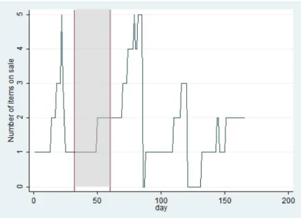
Table 3 reports the results of four different regressions. In columns (1) and (2) the dependent variable is the level of sales of Brand A, while in (3) and (4) it is the logarithm of this level in such a way that coefficients can be interpreted as percentage changes.5 Columns (2) and (4) contain the battery of prices of all the thirteen items that can be considered as substitutes of Brand A. The vector of prices is instead summarized by a single variable describing the number of items on discount in columns (1) and (3). Figure 2 summarizes the pattern of this proxy.
Seasonality in the sale pattern of Brand A, both during the week and in different period of the year, is captured well by the total sales of mozzarella cheese that are strongly significant. As expected, prices of (some) substitutes are significant, like the proxy about the number of items on sale.6
Note: The shadowed area corresponds to the treatment
Figure 2: Number of Items on Discount Every Day
Removing the .99 price ending apparently induces a sizeable and significant average increase of daily sales in all the specifications. This finding seems to
5One observation is lost with the logarithm of sales because the quantity sold is equal to zero. 6Virtually identical results are obtained using a proxy that besides the number of items on sale
internalizes the magnitude of the price changes as well.
confirm what emerges from descriptive statistics, namely that not only .99-ending prices may be ineffective in increasing sales, but that they could also have an opposite effect. A possible interpretation of this counterintuitive result is that consumers use the price as a proxy for the quality of the good. When the price is €.99 consumers probably perceive Brand A as the more expensive within the low-price mozzarella cheeses. In contrast, when the low-price is €1.01 Brand A becomes the cheapest within the medium-price mozzarella cheeses. Although interesting, this interpretation cannot be easily accepted because the estimated specification is not fully convincing.7
Note that sales of Brand B, as well as its price, are never significant as an explanatory variable, meaning either that no unobservable shock occurred in the period analysed, something quite hard to believe, or that Brand B turns out to be a poor control, thereby casting some shadow on the goodness of this specification. If sales of Brand B do not properly control for common shocks that could confound the results we cannot interpret the results as a causal effect. Moreover, this caveat always applies in case of asymmetric shocks regardless of the goodness of Brand B as a control.
What this specification says is that sales of Brand A display a significant increase at the time of the treatment controlling for what happens to the sales of the closest substitute, to the prices of the other substitutes, and to total sales of mozzarella cheese. What follows is a counterexample showing how sales of Brand A could increase relative to the other substitutes due to asymmetric shocks unrelated to the .99 price. Consider first that in this specification sales of mozzarella cheeses other than Brand A and B are regarded as exogenous, but they are clearly not. Sales of every Brand are affected by the prices of all substitutes. It is true that in this multivariate framework we control for the prices of the substitutes, or alternatively for the number of items on discount, but the same price shock can have different effects on the quantity sold of two brands because their cross-elasticity differs. Note that if all the brands react in the same way to variations of the prices of substitutes, changes in quantities would be perfectly collinear. In contrast, if a substitute of
7Such an effect cannot be generalized, since it might hold only when the change in the leftmost digit
is enough to make the consumers perceive the price as being representative of a different quality of the good. For instance, the same price variation from €.99 to €1.01 applied to a bottle of wine would not change the impression that the quality of the wine is very bad.
Brand A reacts less on average to the same price discount of a third item, higher average prices of the third item during the period of the treatment could be associated with higher relative sales of Brand A regardless of having removed the .99-ending price. Figure 2 is consistent with such an interpretation because during the treatment (gray area in the graph) fewer items than the average were on discount.
Note that in the example above whether Brand B fails to capture this mechanism because it is a poor control or instead because it is characterized by a different cross-elasticity does not make any difference. Of course, in the first case additional problems would arise because common shocks could also confound the results.
Summarizing, the specification used in this section cannot account for some subtle additional factors that could affect the results. The next section presents a more general framework, capable of endogenously accounting for what happens to the sales of all the fourteen brands, as well as of controlling for common shocks that could have instead confounded the result of the treatment in the previous specification.
3.2 Sales of Brand A: A Differences in Differences Approach
The so-called differences in differences (DID) method is commonly used in econometrics to measure the effect of a treatment. The idea is always that it is necessary to subtract everything that can happen at the same time of the treatment and that could otherwise confound the results. Towards this goal the DID uses a control group and compares both groups before and during a treatment, assuming that all the other shocks are common. Hence, if the treatment is significant, it must show up not only comparing the treated before and after the treatment, but also comparing the treated with the control group.
The difference with respect to the previous section is that in this case the behaviour of the control group is not treated as exogenous. In contrast, it is assumed to be a function of the same variables used to explain the pattern of the treated.
In this experiment there are thirteen brands that can be considered as substitutes of Brand A (including Brand B), but they are rather different from different points of view (level of sales, characteristics, etc.). Therefore, it seems inappropriate to
consider them as a homogeneous group, and a battery of dummy variables is included in order to allow for some heterogeneity within the control group. For the sake of simplicity the dummies relative to the other brands are grouped in the vector called –A in what follows. The dummy variable that refers to Brand A plays instead the role of the treated group.
The variable T captures possible shocks common to the treated and to the control group, i.e. everything that happened to the whole sample at the same time of the experiment. The effect of the treatment is instead measured by the interaction between A and T, because it captures the change in the dependent variable Y due to whatever characterizes only the treated group and only during the period of the treatment.
The estimated specification is therefore the following:
Yi = α0 (-A) + α1 A + α 2 T + α 3 A*T + α 4 X + εi,
where:
Yi = Daily sales of every brand I,
-A = A vector of dummies for every brand different from A, A = Dummy variable for Brand A,
T = Time dummy equal to one for the period of the treatment, A*T = Interaction term between the two dummies above, X = Vector of controls (prices, total sales).
The battery of daily prices of all brands is included in the vector of controls X allowing for different individual reactions, i.e. interacting the vector of prices with the brand dummies. This would imply that 142 variables should be included, but twelve have been excluded using the quasi-likelihood under the independence model criterion (QIC) (Pan 2001; Cui 2007). Finally, the vector of controls contains the total daily sales of mozzarella cheese in the store like in the previous Section.
Two main differences characterize this specification as compared to that in the previous section. First, the sales of all the substitutes are now endogenously explained by the independent variables allowing for different reactions to the same price changes. Second, confounding factors that concern the whole sample at the
same time are now captured by the dummy T. The effect of removing the .99 price is instead measured by the interaction coefficient α3.
Since the Wooldridge test strongly rejects absence of autocorrelation (Wooldridge 2002; Drukker 2003) the estimated OLS coefficients of the dynamic panel would deliver inconsistent estimates. For this reason Table 4 reports the results of two different regressions of a model in which the disturbance term is first-order autoregressive (Baltagi and Wu 1999).
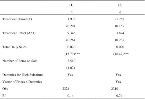
Table 4: Differences in Differences Analysis of Daily Sales of All Brands
(1) (2)
q q
Treatment Period (T) 1.936 -1.263
(0.20) (0.15)
Treatment Effect (A*T) 9.346 3.874
(0.26) (0.23)
Total Daily Sales 0.020 0.020
(15.79)*** (16.47)***
Number of Items on Sale 2.510
(1.07)
Dummies for Each Substitute Yes Yes
Vector of Prices x Dummies Yes
Obs 2324 2310
R2 0.14 0.74
Fixed effects linear model with an AR(1) disturbance Absolute value of t statistics in parentheses
*significant at 10%; **significant at 5%; *** significant at 1%
Column (1) includes the proxy tracking the daily number of items on discount. Column (2) contains the whole battery of prices interacted with the level dummies, i.e. allowing cross-elasticities to differ for every brand, although they are not reported in details to save space. In both cases the dependent variable is the daily quantity sold by every brand.8
8Logarithms are not used in this model because many values equal to zero would generate a lot of
missing values that could bias the results because they are not at random.
Results differ considerably from those of the previous section. The interaction term becomes not significant, meaning that removing the .99-ending price did not determine a change in the sales of Brand A relative to what happens to the other items once we partial out the effect of group and time controls. The coefficient α2 is
also not significant meaning that there is no other common shock specifically affecting the sales of the 14 brands analyzed at the time of the treatment. The total sales of the 51 types of mozzarella cheese are instead strongly significant, capturing the weekly business cycle of the store as well as any other shock that is common to all these 51 items. Note further that controlling for the cross-elasticity of the items boosts the explanatory power of the model. Hence, results are consistent with a higher price-elasticity of the demand for Brand A driving the relative increase of sales during the treatment, when prices of the substitutes are on average higher. Once the different reactions to price changes are taken into account, Brand A does not display significantly higher sales when the .99-ending price is removed.
4
□
Conclusion
The paper investigates the effect of .99 price endings on consumer demand by means of an experiment in which the price in a supermarket of two local brands of mozzarella cheese have been modified in a controlled manner.
When the .99-ending price is removed, a counterintuitive increase of sales emerges from descriptive statistics as well as in multivariate framework in which only the sales of the treated item are used as a dependent variable while controlling for the sales of the closest substitute, the price of all the other substitutes, and total sales of mozzarella cheese in the store. If not confounded with other factors, these finding would suggest that another effect should be taken into account when dealing with .99 ending prices, namely that if prices are used as a proxy for the quality of the good the change in the leftmost digit induced by the .99 ending can imply a change in the perceived quality of the good. For instance, when the price is €.99 consumers perceive the item as the more expensive within the low-price mozzarella cheeses. In contrast, when the price is €1.01 it becomes the cheapest within the medium-price mozzarella cheeses.
However, such a counterintuitive effect of the .99-endings price does not survive in a DID model in which also the daily sales of all the relevant substitutes are explained by level dummies, total sales, and all the prices allowing for different reactions. No common shock emerges and the interpretation of the results points toward a different elasticity of demand driving the relative increase of sales of Brand A during the treatment when prices of the substitutes are on average higher. Once the different reactions to price changes are taken into account, the treated item does not display significantly higher sales as compared to its substitutes when the .99 ending price is removed.
These results can be interpreted as further evidence that the .99 price endings can be ineffective in increasing consumer demand. The results are particularly valuable because data have been gathered by means of a field experiment in a natural setting like a supermarket. Results cannot be generalized to all the situations since they can be specific to the type of product analyzed, the direction and the magnitude of the price change, the cognitive load required by the choice and so on. Nevertheless, this contribution adds to the branch of the literature that questions the effectiveness of .99-ending prices, concluding that they do not have sound enough empirical grounds to justify such a widespread use among retailers.
References
Anderson, E. T. and D. I. Simester, (2003), “Effects of $9 Price Endings on Retail Sales: Evidence from Field Experiments,” Quantitative Marketing and
Economics, 1, 93-110.
Baltagi, B. H. and P. X. Wu, (1999), “Unequally Spaced Panel Data Regressions with AR (1) Disturbances,” Econometric Theory, 15, 814-823.
Basu, K., (2006), “Consumer Cognition and Pricing in the Nines in Oligopolistic Markets,” Journal of Economics and Management Strategy, 15, 125-141. Bizer, G. Y. and R. M. Schindler, (2005), “Direct Evidence of Ending-Digit
Drop-Off in Price Information Processing,” Psychology and Marketing, 22, 771-783. Cui, J., (2007), “QIC Program and Model Selection in GEE Analyses,” The Stata
Journal ,7, 209-220.
Drukker, D. M., (2003), “Testing for Serial Correlation in Linear Panel-Data Models,” The Stata Journal, 3, 168-177.
Georgoff, D. M., (1972), Odd-Even Retail Price Endings, East Lansing, MI: Michigan State University.
Ginzberg, E., (1936), “Customary Prices,” The American Economic Review, 26, 296. Hackl, F., M. E. Kummer, and R. Winter-Ebmer, (2010), “99 Cents: Price Points in
E-Commerce,” ZEW Discussion Papers 10-022.
Harrison, G. W. and J. A. List, (2004), “Field Experiments,” Journal of Economic
Literature ,42, 1009-1055.
Hinrichs, J. V., D. S. Yurko, and J. M. Hu, (1981), “Two-Digit Number Comparison: Use of Place Information,” Journal of Experimental Psychology: Human
Perception and Performance, 7, 890-901.
Kalyanam, K. and T. S. Shively, (1998), “Estimating Irregular Pricing Effects: A Stochastic Spline Regression Approach,” Journal of Marketing Research, 35, 16-29.
Levy, D., D. Lee, H. Chen, R. J. Kauffman, and M. Bergen, (2011), “Price Points and Price Rigidity,” The Review of Economics and Statistics, 93, 1417-1431. Pan, W., (2001), “Akaike's Information Criterion in Generalized Estimating
Equations,” Biometrics, 57, 120-125.
Schindler, R. M., (2006), “The 99 Price Ending as a Signal of a Low-Price Appeal,”
Journal of Retailing, 82, 71-77.
Schindler, R. M. and T. M. Kibarian, (1996), “Increased Consumer Sales Response through Use of 99-Ending Prices,” Journal of Retailing, 72, 187-199.
Schindler, R. M. and P. N. Kirby, (1997), “Patterns of Rightmost Digit Used in Advertised Prices: Implications for Nine-Ending Effects,” Journal of Consumer
Research, 24, 192-201.
Stiving, M., (2000), “Price-Endings When Prices Signal Quality,” Management
Science, 46, 1617-1629.
Stiving, M. and R. S. Winer, (1997), “An Empirical Analysis of Price Endings with Scanner Data,” Journal of Consumer Research, 24, 57-67.
Thomas, M. and V. Morwitz, (2005), “Penny Wise and Pound Foolish: The Left-Digit Effect in Price Cognition,” Journal of Consumer Research, 32, 54-64.
Wooldridge, J. M., (2002), Econometric Analysis of Cross Section and Panel Data, Cambridge, MA: MIT Press.