Evaluation of arsenic contamination potential using indicator kriging in the Yun-Lin aquifer (Taiwan)

0048-9697/04/$ - see front matter䊚 2003 Elsevier B.V. All rights reserved. doi:10.1016/j.scitotenv.2003.09.002

Evaluation of arsenic contamination potential using indicator

kriging in the Yun-Lin aquifer

_(Taiwan)

Chen-Wuing Liu*, Cheng-Shin Jang, Chung-Min Liao

Department of Bioenvironmental Systems Engineering, National Taiwan University, Taipei 106, Taiwan, ROC

Received 31 May 2003; accepted 3 September 2003

Abstract

Data on the quality of groundwater obtained from several multi-level monitoring wells indicated that arsenic(As)

concentration far exceeds the drinking water supply standard in the coastal aquifer of the Yun-Lin, Taiwan.In this study, an estimated As probability risk was computed using indicator kriging to assess the As contamination potential of exceeding the drinking water supply standard in the Yun-Lin county.A three-dimensional(3D) spatial variability

model was presented to analyze anisotropically the variation of As concentration using a multi-level threshold indicator variable.This 3D estimator overcomes the scarcity of the data and establishes a vertical correlation of measured As data.The results indicate high As pollution probability in the coastal area and in the Pei-Kang river basin.The highest probability, 0.92, of the As pollution is in the shallow aquifer of the Kou-Hu.The contamination potential of As is primarily within an aquifer depth of 180 m.The contaminated aquifer (-180 m) is not suitable

for supplying drinking water.The contamination potential of As is low at the depths of more than 190 m.However, the probabilities associated with the As pollution still exceed 0.2 in the deep aquifer of four coastal townships of the Yun-Lin, and may pose risks to human health if the groundwater is used for drinking.

䊚 2003 Elsevier B.V. All rights reserved.

Keywords: Arsenic; Contamination potential; Drinking water standard; Complex aquifer; Indicator kriging

1. Introduction

Arsenic _{(As) has been well documented as a} major risk factor for blackfoot disease _{(Shen and} Chin, 1964_{).Blackfoot disease was once common} on the southwestern coast of Taiwan _(Chiou, 1996_{).The residents had used high-arsenic artesian} well water over 50 years (Tseng,

1977).Large-scale studies on the association between arsenic

*Corresponding author.Tel.: q886-2-2362-6480; fax: q 886-2-2363-9557.

E-mail address: lcw@gwater.agec.ntu.edu.tw(C.-W. Liu).

complexes in well water and age-adjusted mortal-ity from diabetes _{(Lai et al., 1994), hypertension}

(Chen et al., 1995) and cancers of the nasal cavity,

lung, liver, bladder, kidney and prostate (Wu et

al., 1989; Chen and Wang, 1990_{) yield mutually} supporting findings.Patients with blackfoot dis-ease had a substantially raised incidence of cancer, after adjustment for cumulative arsenic exposure.

Yen et al. (1980) presented a geological

envi-ronment model to describe the origin of high arsenic concentrations in the shallow sedimentary basin of southwestern Taiwan.Changes in sea

level significantly influence the composition and structure of the geological environment.The sedi-mentary basin is formed by the alternating invasion and retreat of sea water with interlayered forma-tions of marine and non-marine sequences.The marine sequences with fine sediment, ranging from clay, through silt to fine sand have a relatively high arsenic content, which is accumulated and deposited in the formation.Other sources of arsen-ic contamination are associated with the excess use of a wide range of pesticides, herbicides and agro-fertilizers(Li et al., 1979).The current

drink-ing water supply standard of As in Taiwan is 50

mgyl—much lower than the background As

con-centration level _{(200–2500 mgyl) in the Yun-Lin} area.Groundwater has been abundantly used as an alternative to surface water, especially in the south-western coastal region, such as in the Yun-Lin, where surface water resources are severely defi-cient, due to the high demand for domestic, irri-gation, aquacultural and industrial utilization.As may be directly taken up by drinking water, dam-aging human health; it may also indirectly enter the food-chain through various paths and poses a risk to human health.In 2001, the soil and ground-water remediation act enforced 25 mgyl and 250 mgyl stringent standards for groundwater within

and outside protected areas from which drinking water is supplied, respectively.

The spatial distribution of contaminated ground-water commonly exhibits some heterogeneity. However, only a small proportion of in-situ data can be analyzed in a field investigation, due to time and cost constraints.Consequently, sparse measured data contain considerable uncertainty. Geostatistics are widely used to estimate the spatial variability and distribution of field data with uncer-tainty.Indicator kriging is the most commonly used non-parametric geostatistical method.Indica-tor kriging makes no assumptions on the underly-ing invariant distribution, and 0;1 indicator transformation of data make the predictor robust to outliers(Cressie, 1993).At an unsampled

loca-tion, the values estimated by indicator kriging represent a probability that is less than a specified threshold.That is, the expected value at the loca-tion derived from indicator data is equivalent to the cumulative distribution function of the variable

(Smith et al., 1993).Indicator kriging has been

frequently applied to the pollution of soil by heavy metals.For example, Smith et al._{(1993) and} Oyedele et al. _{(1996) used multivariate indicator} kriging to analyze the quality of soil; Lin et al.

(2002) applied indicator kriging to delineate the

variation and pollution sources of heavy metals in agricultural land; Juang and Lee (1998),

Castrig-nano et al.` (2000) and van Meirvenne and

Goo-vaerts (2001) adopted multi-level-threshold indicator kriging to estimate the probability distri-bution of heavy metal pollution in the field.Geos-tatistical indicator methods have also been applied in the lithological classification of rocks(McCord

et al., 1997; Fogg et al., 1999_{) and in the} estima-tion of contaminaestima-tion probability in groundwater aquifers_{(Istok and Pautman, 1996).}

Methods for assessing the vulnerability of aqui-fers are typically divided into three groups: ₍₁₎ overlay and index methods, _{(2) methods that} involve process-based simulation models, and ₍₃₎ statistical methods (NRC, 1993).Vulnerability

assessments generally include uncertainty.The probabilitic outcomes indicate the unreliability of the assessment.Furthermore, the occurrence prob-abilities of contamination can be used to reveal the relative contamination potential under uncer-tainty conditions of sparse measured data.

This work applies indicator kriging to assess the contamination potential of As in the Yun-Lin.The As formation and source in the Yun-Lin aquifers are highly associated with sedimentary environ-ments.The study assumed that the As distributions of three aquifers were vertically correlated owing to similar formation environments.A three-dimen-sional _{(3D) spatial variability and distribution of} As probabilistic risk and its associated contami-nation potential are constructed and assessed using multi-level-threshold indicator kriging.The deter-mined As contamination probability is overlaid on a township map of the Yun-Lin county, using a geographic information system(GIS), to delineate

the varying contamination potential and the con-tamination sources of As.The established spatial probability risk distribution is a useful guide that helps the water service company to place wells to meet the water quality standards of various water supply needs.

Fig.1.Locations of twenty townships in the Yun-Lin county, Taiwan. 2. Study area

The Yun-Lin County is located in the southern part of the Chou-Shui River alluvial fan _(Fig.1). The area is enclosed by the Taiwan Strait to the west, the Central Mountain to the east, the Chou-Shui river to the north and the Pei-Kang river to the south.Chou-Shui and Pei-Kang are the two major rivers that flow through the area.The area is approximately 1000 km , and extends 48 km2

from east to west and 24 km from north to south. The average annual precipitation is 1417 mm. Rainfall is concentrated in the five-month period from May to September.

Agriculture is the primary source of revenue in the Yun-Lin.The industrial sector has grown rap-idly, causing the average income of farmers to fall considerably below that of workers in other sec-tors.Therefore, many farmers have converted their croplands into fishponds to boost earnings.A large amount of groundwater has been extracted from

the aquifer to supply these fishponds.The extrac-tion has caused severe land subsidence, seawater intrusion, flooding and deterioration of the sur-rounding environment (Tsao and Wang, 1984;

Shen, 1989; Geng et al., 1994).

Between 1992 and 1998, the government imple-mented a 7-year comprehensive groundwater mon-itoring network plan to investigate the hydro-geological characteristics of the main groundwater system in Taiwan.The new groundwater-monitor-ing network in the Chou-Shui River alluvial fan was quickly implemented.It includes 77 hydro-geological investigation stations and 188 ground-water-monitoring wells in different aquifers

(Taiwan Sugar Company, 1997).A

hydrogeologi-cal study revealed that the alluvial fan was of the late Quaternary age and was partitioned primarily into proximal-fan, mid-fan and distal-fan areas.In the subsurface hydrogeological analysis to a depth of approximately 300 m, the formation can be divided into six interlayered sequences, including

Fig.2.Conceptual hydrogeological profile in the Yun-Lin county, Taiwan along transect A–A9 in Fig.1.

Table 1

Statistics of measured As concentrations in groundwater from 1999 to 2001 in the Yun-Lin county, Taiwan

Statistics Year

1999 2000 2001

Well number 107 107 35

Average(mgyl) 53.9 65.9 168

Standard deviation(mgyl) 91 120 200

Skewness 2.99 3.00 2.34 Minimum(mgyl) -10 -10 20 Maximum(mgyl) 570 640 830 Percentile(mgyl) 10 -10 -10 45 20 -10 -10 50 30 -10 -10 58 40 10 -10 75 50 17 16 87 60 27 25 116 70 40 46 152 80 78 94 190 90 143 163 590

three marine sequences and three non-marine sequences, in the distal-fan and the mid-fan areas. Generally, the non-marine sequences, with coarse sediment, ranging from medium sand to gravel of high permeability, can be considered as aquifers, whereas the marine sequences with fine sediment, can be considered as aquitards _(Fig.2).The hydrogeological formation of the proximal-fan, which consists entirely of gravel and sand, is regarded as an unconfined aquifer and an important groundwater recharge area _{(Central Geological} Survey, 1999).

The south side of the Chou-Shui River alluvial fan has 107 monitoring wells, including 23 wells in aquifer 1 with depths of less than 50 m, 54 wells in aquifer 2 with depths between 60 and 180 m, and 24 wells in aquifer 3 with depths between 190 and 280 m.Additionally, six wells have depths of more than 280 m.

The Taiwanese Water Supply Company had a total of 235 groundwater right permits in the Yun-Lin, issued by the Water Resources Agency in 2002.The averaged water quantity permit was 0.03 m3ys for domestic use, clearly indicating that

groundwater remains a major resource for drinking in the Yun-Lin.

From 1999 to 2001, the Taiwan Sugar Company

(2001) undertook three groundwater quality

sur-veys in the Chou-Shui River alluvial fan; the most recent survey in 2001 focused only on the wells in which the concentration of As was high.The

survey analyzed 31 water quality items including the concentration of As.The measured As concen-trations in the Yun-Lin are typically higher than those in the Chang-Hwa.This investigation thus focuses on assessing the As contamination poten-tial in the Yun-Lin.Table 1 presents the descriptive statistical results of data from three groundwater quality surveys.The As concentrations exhibit a positively skewed distribution with mostly low As concentrations.Approximately 40% of the As con-centrations were below the detection limit (-10 mgyl) in the first two surveys, and the maximum

As concentration increased steadily with time. High As concentrations were found in the west and southwest shallow monitoring wells _(Fig.3).

Fig.4 plots the vertical distribution of measured As concentrations.The highest As concentration is at a depth of 40 m below sea-level.Notably, the As concentration of a few samples taken at a depth of more than 300-m depth exceeded the drinking water limit, suggesting that the use of deep ground-water still poses a risk to human health.The correlation coefficient of measured As concentra-tions in 1999–2000, and in 2000–2001 are 0.85 and 0.93, respectively, suggesting that the variation of As concentration is mild.The As concentrations in 2000 were slightly higher than those in 1999;

Fig.4.Vertical distribution of measured As concentrations in 2000.

therefore, the As concentrations measured in 2000 are adopted herein to assess the contamination potential in the Yun-Lin.

3. Method

3.1. Variogram analysis

Geostatistical methods are based on the region-alized variable theory that states that variables in an area exhibit both random and spatially struc-tured properties _{(Journel and Huijbregts, 1978).} The geostatistical spatial assumption is generally made that the regionalized variable is second-order stationary.A geostatistical variogram of the data should first be determined.The variogram quanti-fies the spatial variability of random variables between two sites.In practice, an experimental variogram, gˆ_(h), is computed as,

N h_{( )} S W 1 T wx z|2T ˆ U X g

Ž .

8

Ž

.

Ž .

Ž .

where gˆ_(h)denotes the variogram for an interval lag distance class h; N_{(h) represents the number}

of pairs for an interval lag distance class h, and z_{(u ) and z(u qh) are the values of the regionali-}i i

zed variables of interest at locations u and u qh,i i

respectively.

The experimental variogram, gˆ_(h), is fitted a theoretical model, g(h), such as spherical,

expo-nential, or Gaussian, to determine three parameters, including the nugget effect _{(c ), the sill (c) and}o

the range_{(a).These models are defined as follows}

(Isaaks and Srivastava, 1989). Spherical model: 3 w z S B E_h B E_h Tg_{(h)sc q 1.5o}

x

|

x

|

x

x

||

Variogram can be computed in different direc-tions to detect any anisotropy of the spatial varia-bility.An anisotropic model generally includes geometric anisotropy and zonal anisotropy.The former type of anisotropy yields variograms having the same structural shape and maximum variability

(sill) but a direction-dependent range for the

spa-tial correlation.The latter type, however, is defined by sills varying with direction_{(Goovaerts, 1997).} The study area is a multi-layered aquifer system. The spatial scale in the horizontal direction is very different from that in the vertical direction: the distance between pairs of groundwater monitoring wells in the horizontal direction exceeds 3 km, whereas the largest difference between two meas-urements of As concentration in the vertical direc-tion is less than 0.35 km. This work thus uses a 3D spatial pairing strategy for calculating an exper-imental variogram in the same aquifer_{(Type I), in} different aquifers _{(Type II) and in different wells} at the same investigation station in the vertical direction _{(Type III) (Fig.5).The first two types}

Fig.5.Three searching pair types for calculating experimental variograms (enlarging in the vertical direction).MSL is the

mean sea level.

(Types I and II), whose maximum angles between

pair vectors and the horizontal direction are under 78, are defined as approximately horizontal and as large-scale searching pairs.

The third type_{(Type III) is defined as a vertical} and small-scale search pair.The 3D spatial varia-bility has been frequently used in estimating the hydraulic conductivity distribution (Hess et al.,

1992; Rehfeldt et al., 1992; Boman et al., 1995; Eggleston et al., 1996; Nakaya et al., 2002; Liu et al., 2002).The 3D analysis differentiates the

hor-izontal direction (large-scale) from the vertical

direction (small-scale) zonal anisotropy using a

nested variogram.Geometric anisotropy is per-formed to evaluate the horizontal anisotropic var-iability.The full 3D anisotropy analysis searches for pairs in a spiral along three principal axes, overcoming the sparse measured data in each aquifer, increasing the vertical correlation among measured data, and yielding a small estimation error _{(Liu et al., 2002).}

3.2. Indicator kriging

Indicator kriging is a non-parametric geostatist-ical method for estimating the probability of

exceeding a specific threshold value,z , at a givenk

location.In indicator kriging, the stochastic varia-ble,Z_{(u), is transformed into an indicator variable}

with a binary distribution, as follows:

S_{1, if Z(u)Fz , ks1,2,...,m}

T k

U

I_{(u;z )s}k T . ₍₅₎

V0, otherwise

The expected value ofI(u; z ), conditional to nk

surrounding data, can be expressed as,

w x

_µ

_∂

E I(u;z ±(n)) sProb Z(u)Fz ±(n)k k

s_{F(u;z ±(n))k (6)} P(u;z ±(n))s1yF(u;z ±(n))k k (7)

where F(u; z N(n)) is the conditional cumulativek

distribution function ofZ(u)Fz , and P(u; z N(n))k k

is the probability that Z_{(u))z .At an unsampled}k

location, u , an estimation must utilize indicator0

kriging and the indicator estimator, I*_{(u ; z ),}0 k

according to,

n

I*_{(u ;z )s}0 k

8

where I(u ; z ) represents the values of the indi-j k

cator at measured locations, u , js1,2,«,n, andj

lj is the weighting factor ofI(u ; z ) in estimatingj k

I*(u ; z ).Indicator kriging estimation must be0 k

unbiased and with minimum estimation error var-iance; that is,

w x

E I*(u ;z )yI(u ;z ) s00 k 0 k (9)

w x

VarI*(u ;z )yI(u ;z )0 k 0 k is minimum. ₍₁₀₎ The weights, lj, are solution of the following system, S n _{l(z )g (u yu ;z )ym(z )sg (u yu ;z )} j k I i j k k I i 0 k

8

T

T

8

where m(z ) is the Lagrange multiplier, g (u yk I i

indicator variables at the ith and jth sampling

points; gI_{(u yu ;z ) is the variogram value}i 0 k

between the indicator variables at theith sampling

point u .0

As concentration is the spatial attribute of inter-est.The sampling frequency distribution of the contaminant generally exhibits a severe, positive bias, which makes non-parametric estimation method more appropriate.The use of a single threshold cannot accurately describe the probabil-ity distribution.Goovaerts (1997) suggested the

use of 5;15 thresholds in indicator kriging to estimate the spatial variable.However, the proba-bility estimate at each threshold may exceed unity or be smaller than zero, and order-relation devia-tion may occur, violating the monotonic increase in the conditional cumulative distribution function. This investigation sets up six thresholds to deter-mine the conditional cumulative distribution func-tion at each grid point.

3.3. Cross-validation

In a cross-validation procedure, measured data are dropped one at a time and re-estimated from some of the remaining neighboring data.Each datum is replaced in the data set once it has been re-estimated.The two parameters are computed as follows_{(Isaaks and Srivastava, 1989; Deutsch and} Journel, 1998_). N 1 _{w * z} x | KMEs

8

Ž

.

Ž

.

Ž

.

Ž

.

8

Ž

.

where I*(u ;z ) and I(u ;z ) are the estimated andi k i k

measured values at the ith location, respectively, N is the number of measured wells, and s(u ;z )2

i k

is the kriging variance.The KME _{(kriging mean} error_{) and MSSE (mean square standard error),} which are close to zero and one, respectively, denote the best fitting models and parameters of variograms.

4. Results and discussion

This work used the gamv and ik3d codes in GSLIB (Deutsch and Journel, 1998) to compute

the experimental variogram and indicator kriging. The estimates of As contamination were analyzed using the SPSS statistical package (SPSS Inc.,

1998).

4.1. Variogram analysis

The As concentrations at the 50(1st), 60 (2nd),

70 (3rd), 80 (5th) and 90 (6th)% points on the

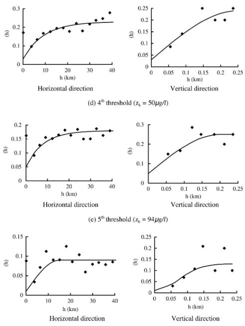
percentage frequency distribution of As concentra-tion measured in 2000, were used as the first five threshold values.The drinking water supply stan-dard As concentration of 50 ppb is used as the fourth threshold value, and corresponds to 72% of the percentage frequency distribution of the As concentration data measured in 2000.The first five threshold values based on the measured As con-centration frequency distribution were used to derive the conditional cumulative distribution func-tion at each estimated grid point.This investigafunc-tion is mainly concerned with the fourth threshold value, based on the drinking water supply standard. Employing a least squares method to fit a variogram yields a model with the least fitting errors _{(Cressie, 1985).An omnidirectional} vario-gram is first used to analyze the horizontally varying structures of As concentration.A lag increment of 3 km is used to obtain a stable variogram structure _{(Fig.6).The spherical and} exponential models give the best fits.Table 2 specifies the fitting parameters of these models. The fitted ranges, sills and nugget effects are 15;40 km, 0.08;0.25 and 0.01;0.12, respec-tively.The large-scale searching pairs in the hori-zontal direction are of Types I and II.The first pair in the horizontal variogram whereh is

approx-imately 0.1;0.2 km yields a large variability. This pair represents a small-scale variability and should only be included to the variogram in vertical direction_{(Type III).The first pair is thus excluded} from the horizontal large-scale variogram analysis. Lag increments of 0.025 and 0.03 km are used to

Fig.6.Experimental variograms indicator of As concentration and the fitting of theoretical models in horizontal and vertical directions for six thresholds.(Omni-directional variogram is applied to horizontal direction).

establish a stable variogram in the vertical direc-tion on a small scale _{(Fig.6).The Gaussian and} spherical models yield the best fitting.The nugget effects of the nested variogram are mainly inferred from the vertical variogram, which typically has the excellent spatial resolution.The fitted ranges

and sills are 0.2;0.35 km and 0.12;0.21, respectively.

To account for anisotropy along the horizontal direction, variograms are computed in various directions, separated by successive clockwise rota-tions of 158 from north to south.The directional

Fig.6(Continued).

experimental variogram searches for pairs with an angular tolerance of 308.However, experimental variograms inevitably oscillate at a specific corre-lation distance because insufficient data pairs and non-uniformly distributed wells are involved.

The models that were fit to omnidirectional variograms were also used to model the anisotropic

variability.The determined directions of maximum variability for each threshold range from N to N308E, and is N for four thresholds.The aniso-tropic ratio _{(maximum rangeyminimum range) is} approximately 1.88;3.18_{(Table 2).}

Table 2 also lists cross-validation results to examine the validity of the fitting models and

Table 2

Fitted parameters of the theoretical variogram model for six thresholds of As indicator variable

Threshold Direction Model type Nugget Sill Range Max. Min. Anisotropic Max. KME MSSE effect (km) range range ratio variability

(km) (km) direction 1st H* Spherical 0.09 0.2 30 40 20 2 N y0.009 1.18 V** Gaussian 0.09 0.14 0.35 – – – – 2nd H Spherical 0.08 0.25 40 45 24 1.88 N308E 0.008 0.99 V Gaussian 0.08 0.18 0.35 – – – – 3rd H Spherical 0.12 0.14 40 45 18 2.5 N158E 0.009 0.91 V Spherical 0.12 0.14 0.25 – – – – 4th H Exponential 0.03 0.2 28 35 15 2.33 N 0.009 0.79 V Spherical 0.03 0.21 0.25 – – – – 5th H Exponential 0.05 0.13 24 35 11 3.18 N 0.006 0.75 V Spherical 0.05 0.2 0.2 – – – – 6th H Spherical 0.01 0.08 15 22 10 2.2 N 0.004 1.05 V Gaussian 0.01 0.12 0.3 – – – – *H: horizontal, **V: vertical

parameters of variograms.The KMEs range from

y_{0.009 to 0.009 and the MSSEs range from 0.75}

to 1.18.The KMEs are close to zero.In a cross-validation procedure, Chiles and Delfiner` ₍₁₉₉₉₎ proposed the MSSE with a tolerance interval of

(i.e. w0.59, 1.41x).The MSSEs of this

y

1"3 2yN

study fall within the proposed tolerance range.

4.2. Indicator kriging estimation

Indicator kriging was used to estimate the prob-ability of As contamination, based on 3D anistrop-ic variogram models.Each aquifer was horizontally discretized into a grid of 27=19 cells, with a 2 km spacing.The elevation of the aquifers varied irregularly, so the grid used in the estimation was set by the midpoints of each aquifer in the vertical direction.

The probability of contamination (P(u;50)) is

mapped for the three aquifers in Fig.7.The southwestern coastal aquifer has a high probability of contamination by As, whereas the banks of the Chou-Shui River have a low probability, especially in the proximal-fan area.The highest measured As concentration (640 mgyl) was in aquifer 1 of the

Ming-Der monitoring well in the western Yun-Lin. However, the highest As contamination probability determined using indicator kriging appears in the south of the Ming-Der monitoring well.Indicator kriging compares the set threshold value with the

measured As concentration and then transforms the measured concentration to 0 or 1.The largest threshold value used in this study is 163 mgyl,

corresponding to 90% of the cumulative frequency distribution of the measured As concentrations.If the measured As concentrations exceed the 163

mgyl threshold, then the indicator variables are all

set to zero and cannot reflect the extremely high measured As concentration, such as of 640 mgyl.

Notably, Goovaerts (1997) stated that measured

data above 90% of the cumulative frequency dis-tribution cannot be suitably set as thresholds for indicator kriging.Moreover, the kriging method applies the weighted moving-average technique to estimate the unknown concentrations at the neigh-boring points.If the estimated concentrations all exceed the threshold set in adjacent regions, then indicator kriging assigns a high probability of contamination in the region of interest.The As concentration in the points that neighbor the Ming-Der monitoring well is relatively low, reducing the probability of contamination in the vicinity.Fur-thermore, because the 3D anisotropic model was used to estimate the neighboring As concentrations in the deep aquifer, the weighted moving-average technique uses the high As concentrations in the upper aquifers to calculate contamination proba-bility in aquifer 3.Indicator kriging estimates a 0.2;0.6 probability of As contamination in the southwestern area of aquifer 3, only one or two

Fig.7.Estimated probability distribution of the As concentration that exceeds the standard of drinking water supply in the Yun-Lin county, Taiwan using indicator kriging.

As concentrations in the monitoring wells exceed the standard for the drinking water supply.

The statistical analysis of the estimated proba-bilities of As contamination of 513 cells in the

three aquifers indicates that the average and max-imum contamination probability of contamination of aquifers 1, 2 and 3 are 0.34 and 0.97; 0.28 and 0.84, and 0.15 and 0.67, respectively _{(Table 3).}

Table 3

Statistics of estimated probability of As concentrations exceed-ing the standard of drinkexceed-ing water supply by indicator krigexceed-ing

Statistic Aquifer 1 2 3 Mean 0.34 0.28 0.15 Median 0.23 0.22 0.12 Standard deviation 0.30 0.25 0.14 Skewness 0.54 0.56 1.00 Minimum 0.00 0.00 0.00 Maximum 0.97 0.84 0.67 Table 4

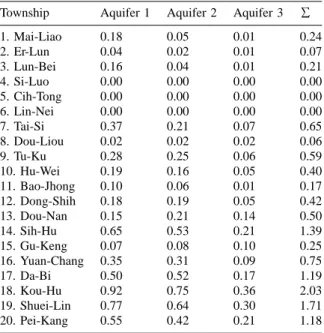
Estimated As contamination potential order of 20 townships in the Yun-Lin county, Taiwan

Township Aquifer 1 Aquifer 2 Aquifer 3 8

1. Mai-Liao 0.18 0.05 0.01 0.24 2. Er-Lun 0.04 0.02 0.01 0.07 3. Lun-Bei 0.16 0.04 0.01 0.21 4. Si-Luo 0.00 0.00 0.00 0.00 5. Cih-Tong 0.00 0.00 0.00 0.00 6. Lin-Nei 0.00 0.00 0.00 0.00 7. Tai-Si 0.37 0.21 0.07 0.65 8. Dou-Liou 0.02 0.02 0.02 0.06 9. Tu-Ku 0.28 0.25 0.06 0.59 10. Hu-Wei 0.19 0.16 0.05 0.40 11. Bao-Jhong 0.10 0.06 0.01 0.17 12. Dong-Shih 0.18 0.19 0.05 0.42 13. Dou-Nan 0.15 0.21 0.14 0.50 14. Sih-Hu 0.65 0.53 0.21 1.39 15. Gu-Keng 0.07 0.08 0.10 0.25 16. Yuan-Chang 0.35 0.31 0.09 0.75 17. Da-Bi 0.50 0.52 0.17 1.19 18. Kou-Hu 0.92 0.75 0.36 2.03 19. Shuei-Lin 0.77 0.64 0.30 1.71 20. Pei-Kang 0.55 0.42 0.21 1.18

The shallow aquifers 1 and 2 have a higher probability of As contamination than the deep aquifer 3.

4.3. As contamination potential of twenty townships

The Arcview 3.2 _{(ESRI, 1998) GIS map of 20} townships in the Yun-Lin was overlaid on the As probability maps, to determine the average proba-bility of As contamination potential in each town-ship.The As contamination potential was specified using five levels.The first level denotes an As contamination probability of less than 0.2 corre-sponding to unpolluted groundwater.If the As contamination probability exceeds 0.2, then the groundwater is considered polluted and is not suitable for supply as drinking water.The ranges of probabilities of As contamination in the second, third, fourth and fifth levels are 0.2;0.4, 0.4;0.6, 0.6;0.8, and 0.8;1.0, respectively. A high level of the contamination potential corresponds to a high As contamination probability and a high risk to human health.

Table 4 shows the As contamination potential of 20 townships from high to low, and Fig.8 depicts the spatial distribution of As contamination potential.The contamination potential in aquifer 1 in Kou-Hu reaches the highest fifth level and the corresponding As contamination probability is 0.92. Drinking groundwater from aquifer 1 in Kou-Hu is an immediate and high risk to human health. In four places, including aquifer 2 in Kou-Hu, aquifers 1 and 2 in Shuei-Lin, and aquifer 1 in

Sih-Hu, the As contamination potential reaches the fourth level.In five places, including aquifer 2 in Sih-Hu, aquifers 1 and 3 in Da-Bi, aquifers 1 and 2 in Pei-Kang, the As contamination potential reaches the third level.In 11 places, it reaches the second level and in all the remaining places, it reaches the first level.Notably, the As contami-nation potential of all three aquifers in Si-Luo, Cih-Tong and Lin-Nei are zero, representing no As contamination.

The high contamination potential of As is con-fined to the southwest coastal area and along the Pei-Kang River banks.The township of Kou-Hu, with the highest As contamination potential, is located in the junction between the southwest coastal area and the Pei-Kang River bank.Results indicate that the probability of contamination of aquifer 1 exceeds that of aquifer 2, and that aquifer 3 is the least likely to be contaminated, among the three aquifers.There are only four southwestern townships of the Yun-Lin where their aquifer 3 reach the second level of As contamination potential.

Fig.8.Estimated contamination potential of As concentration exceeding the standard of drinking water supply in 20 town-ships of the Yun-Lin county, Taiwan.

5. Conclusions

High As contamination is detected throughout the coastal aquifer of the Yun-Lin, Taiwan. Groundwater quality data, obtained from

multi-level monitoring wells, indicated that the As con-centration far exceeds the drinking water supply standard and poses a serious threat to public health. This work adopted indicator kriging to estimate the probabilistic risk of As pollution in the Yun-Lin area.A 3D variogram model analyzed the As concentration probability, using an indicator vari-able with multi-level thresholds.The method solved the problem of data scarcity, increased the number of searching pairs for calculating an exper-imental variogram in the vertical direction, and provided multi-level thresholds in the probability estimation of contamination.

The estimates reveal that the high As pollution probability is distributed in the southwest coastal area and along the Pei-Kang River bank.Among 20 townships of the Yun-Lin county, Kou-Hu has the highest As contamination potential in its shal-low aquifer.Shalshal-low aquifers 1 and 2 (depth-180 m_{) have high As contamination potentials and} cannot be used to supply drinking water.The deep aquifer 3 _{(depth)190 m) has a low As} contami-nation potential and may be used for supplying drinking water, except in Kou-Hu, Sih-Hu, Shuei-Lin and Pei-Kang where the As contamination potentials are at the second level and still represent a risk to human health.

Acknowledgments

The authors would like to thank the National Science Council of the Republic of China for financially supporting this research Under Contract Nos.NSC 90-2313-B-002-322 and NSC 91-2313-B-002-270.

References

Boman GK, Molz FJ, Guven O.An evaluation of interpolation¨ methodologies for generating three-dimensional hydraulic property distributions from measured data.Ground Water 1995;33(2):247 –258.

Castrignano A, Goovaerts P, Lulli L, Bragato G.A geostatist-` ical approach to estimate probability of occurrence of Tuber melanosporum in relation to some soil properties.Geoderma 2000;98:95 –113.

Central Geological Survey.Project of groundwater monitoring network in Taiwan during first stage-research report of

Chou-Shui River alluvial fan.Taiwan: Water Resources Bureau, 1999.p.383

Chen CJ, Wang CJ.Ecological correlation between arsenic level in well water and aged-adjusted mortality from malig-nant neoplasms.Cancer Res 1990;50:5470 –5474. Chen CJ, Hsueh YM, Lai MS, Shyu MP, Chen SY, Wu MM,

Kuo TL, Tai TY.Increased prevalence of hypertension and long-term arsenic exposure.Hypertension 1995;25:53 –60. Chiles JP, Delfiner P.Geostatistics: modeling spatial uncertain-`

ty.New York: John Wiley and Sons Inc, 1999.p.283 –287. Chiou HY.Epidemiologic studies on inorganic arsenic

meth-ylation capacity and inorganic arsenic induced health effects among residents in the blackfoot disease endemic area and Lanyang basin in Taiwan.Doctoral Dissertation, Institute of Epidemiology, College of Public Health, National Taiwan University, Taiwan, 1996: p.8.

Cressie N.Fitting variogram models by weighted least square. Math Geol 1985;17:563 –586.

Cressie N.Statistics for spatial data.New York: Wiley, 1993. Deutsch CV, Journel AG.GSLIB: Geostatistical software library and user’s guide.2nd ed.New York, USA: Oxford University Press, 1998.

Eggleston JR, Rojstaczer SA, Peirce JJ.Identification of hydraulic conductivity structure in sand and gravel aquifers, Cape Cod data set.Water Resour Res 1996;32:1209 –1222. ESRI.Arcview.Redlands, CA: ESRI(Environmental Systems

Research Institute), 1998.

Fogg GE, LaBolle EM, Weissman GS.Groundwater vulnera-bility assessment: hydrologic perspective and example from Salinas Valley, California.Assessment of non-point source pollution in the Vadose zoneAmerican Geophysical Union, 1999.p.45 –61 (Geophysical Monograph 108).

Geng CC, Hsueh CH, Kung CS.Modeling of the groundwater flow and land subsidence in Yun-Chia plain and Yun-Lin offshore industrial area.Conference on Groundwater Research and Quality Protection, Taiwan, 1994: 453–472. Goovaerts P.Geostatistics for natural resources evaluation.

New York: Oxford University Press, 1997.p.259 –368. Hess KM, Wolf SH, Celia MA.Large-scale natural gradient

tracer test in sand and gravel, Cape Cod, Massachusetts 3. Hydraulic conductivity variability and calculated macrodis-persivites.Water Resour Res 1992;28:2011 –2027. Isaaks EH, Srivastava RM.An introduction to applied

geos-tatistics.New York: Oxford University Press, 1989.p.278 – 322.

Istok JD, Pautman CA.Probabilistic assessment of ground-water contamination 2.Results of case study.Ground Water 1996;34(6):1051 –1064.

Journel AG, Huijbregts CJ.Mining geostatistics.San Diego: Academic Press, 1978.

Juang KW, Lee DY.Simple indicator kriging for estimating the probability of incorrectly delineating hazardous areas in a contaminated site.Environ Sci Technol 1998;32:2487 – 2493.

Lai MS, Hsueh YM, Chen CJ, Shyu MP, Chen SY, Kuo TL, Wu MM, Tai TY.Ingested inorganic arsenic and prevalence of diabetes mellitus.Am J Epidemiol 1994;139:484 –492.

Li GC, Fei WC, Yen PY.Survey of arsenical residual level in the rice paddy soil and water samples from different loca-tions of Taiwan.Natl Sci Council Mon, ROC 1979;7(8):798 –809.

Lin YP, Chang TK, Shih CW, Tseng CH.Factorial and indicator kriging methods using a geographic information system to delineate spatial variation and pollution sources of soil heavy metals.Environ Geol 2002;42:900 –909. Liu CW, Jang CS, Chen SC.Three-dimensional spatial

varia-bility of hydraulic conductivity in the Choushui River alluvial fan, Taiwan.Environ Geol 2002;43(1–2):48 –56.

McCord JT, Gotway CA, Conrad SH.Impact of geologic heterogeneity on recharge estimation using environmental tracers: numerical modeling investigation.Water Resour Res 1997;33(6):1229 –1240.

Nakaya S, Yohmei T, Koike A, Hirayama T, Yoden T, Nishigaki M.Determination of anisotropy of spatial corre-lation structure in a three-dimensional permeability field accompoied by shallow faults.Water Resour Res 2002;38(8):10.1029y2001WR000672.

NRC(National Research Council).Ground water vulnerability

assessment: predictive relative contamination potential under conditions of uncertainty.Washington, DC: National Acad-emy Press, 1993.p.42 –63.

Oyedele DJ, Amusan AA, Obi A.The use of multiple-variable indicator kriging technique for assessment of the suitability of an acid soil for maize.Trop Agric 1996;73(4):259 –263.

Rehfeldt KR, Boggs JM, Gelhar LW.Field study of dispersion in a heterogeneous aquifer 3.Geostatistical analysis of hydraulic conductivity.Water Resour Res 1992;28:3309 – 3324.

Shen SB.Study on land subsidence in coastal plains in Yun-Lin area(I).Conference on Land Subsidence, Taiwan, 1989,

pp.191–211.

Shen YS, Chin CS.Relation between blackfoot disease and pollution of drinking water by arsenic in Taiwan.NY: Pergamon Press, 1964.p.175 –182 (Adv Water Pollut Res). Smith JL, Halvorson JJ, Papendick RI.Using multiple-variable

indicator kriging for evaluating soil quality.Soil Sci Soc Am J 1993;57:743 –749.

SPSS Inc.. SPSS BASE 8.0-Application Guide. Chicago: SPSS Inc, 1998.

Taiwan Sugar Company.Establishment and operational man-agement of groundwater monitoring network.Taiwan: Water Resources Bureau, 1997.p.2 –12.

Taiwan Sugar Company.Water quality survey and analysis of groundwater monitoring network.Taiwan: Water Resources Bureau, 2001.p.68 –74.

Tsao YS, Wang JL.A comprehensive study of sea water intrusion for the Yun-Lin aquifer system.Taiwan: Agricul-tural Engineering Research Center, 1984.p.159

Tseng WP.Effects and dose-response relationships of skin cancer and blackfoot disease with arsenic.Environ Health Perspect 1977;19:109 –119.

van Meirvenne M, Goovaerts P.Evaluating the probability of exceeding a site-specific soil cadmium contamination thresh-old.Geoderma 2001;102:75 –100.

Wu MM, Kuo TL, Hwang YH, Chen CJ.Dose-response relation between arsenic well water and mortality from

cancers and vascular diseases.Am J Epidemiol 1989;130:1123 –1132.

Yen FS, Long CN, Lu TH.An environmental model of high arsenic concentration in the groundwater aquifer of Taiwan. J Taiwan Environ Sanitation 1980;12(1):66 –80.