An Automatic Directives-based Parallel Program Generator on PC Clusters

全文

(1)An Automatic Directives-based Parallel Program Generator on PC Clusters Chao-Tung Yang and Wen-Yang Chen High Performance Computing Laboratory Department of Computer Science and Information Engineering Tunghai University Taichung, 407, Taiwan, R.O.C. [email protected]. Abstract. In this paper, we develop a new tool named Automatic Directives-based Parallel Program Generator (ADPPG) for transformation from sequential C source code to parallel one using C with MPI. The main effort in the research is on the parallelism of loops for almost all parallelisms occur in loops. We also introduce loop partitioning into our system. Our system is very straightforward with the technique of message-passing behavior analyzer which is easy to understand but effective. The performance is evaluated and the comparison between ADPPG and hand-rewritten is shown in experimental results. It could be a general-purpose tool to speedup parallel programming or port current sequential programs to parallel architectures. Especially for a beginner to parallel programming, it is a recommended tool to learn more about programming with MPI and more knowledge of loop partitioning. Key words: PC Clusters, MPI, automatic parallel programming, parallel code generator. 1.. Introduction. The computation needed in science field is getting more and more heavier. From the top500 report [1], clustering architecture is believed that it will be the main stream of computation. It is one of the parallel computer platforms with high scalability, high availability and low cost/performance ratio. For these characteristics, clusters are easy to get even self-made for many laboratories performing experiments which taking great part of computation like N-body problem, DNA sequence simulation, weather prediction, nuclear simulation, high-energy physics, etc. Roughly speaking, there are three types of parallel architecture: Shared-Memory Multiprocessor System, Distributed-Memory Multiprocessor System and Clustering System. Within Shared-Memory Multiprocessor System, “one computer” contains not only one processor and each processor shares the same memory by system bus. In other words, all processors have the same memory address space. Sometimes we also call it SMP (Symmetric Multiple Processors). The advantage is all processors share all data such that the communication between each other is very convenient. But it causes some problems of memory sharing: when more than one processor requires writing to memory in the same time, which is first? How many processors can access data in the same memory address concurrently? All these are very complex. Another problem is its scalability is restricted to the system bus bandwidth. Within Distributed-Memory Multiprocessor System, “one computer” contains many processors but each has its own local memory. We can say this system has many processor modules (processor plus local memory). It is so called MPP (Massively Parallel Processors). When communication is needed, they can pass message between each other, of course the network between each module is.

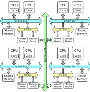
(2) system bus. It is not such convenient for a programmer to write parallel programs when compared with using SMP system. But it has high scalability. The third type is cluster of PCs/Workstations [2, 3, 4]. Many individual PCs/Workstations, in general they are the some type of system architecture, are connected by high-speed network as shown in Fig. 1. As we mentioned, it has high scalability, high availability and low cost/performance ration. We can use message-passing languages to achieve parallel programming in cluster systems. It is getting more and more popular for many laboratories for affordable price. CPU. CPU. CPU. CPU. Cache. Cache. Cache. Cache. System Bus. System Bus. Storage Device. Network Device. CPU. CPU. Cache. Cache. I/O Bus. High Speed Network. I/O Bus. Shared Memory. Network Device. CPU. Cache. Cache. System Bus. I/O Bus. Storage Device. Storage Device. CPU. System Bus. Shared Memory. Shared Memory. Network Device. I/O Bus. Network Device. Shared Memory. Storage Device. Fig. 1. A typical PC Clusters. In message passing, a programmer can achieve parallel programming by three approaches. First, using a new parallel programming language. Second, extending an existing sequential language to handle message passing. Third, using an existing sequential language with a library of external functions for message passing. The third option is the most popular approach being used with one of two specific systems, PVM (Parallel Virtual Machine) [5] or MPI (Message Passing Interface) [6]. Our final aim is to build a parallelizing compiler to convert a program written in C into a parallel program using C with MPI. The first step to our parallelizing compiler is to develop a system that generates a parallel C program with MPI. It can be a general-purpose tool. Especially, for a beginner to parallel programming, it is a recommended tool to learn more about programming with MPI and more knowledge of loop partitioning. The remainder of the paper is organized as follows. In Section 2, some background knowledge about parallelization is presented. In Section 3, details about our system will be given. In section 4, some case studies of experimental results will be shown. The comparison of different methods is also included. Finally, in section 5, we present the conclusions and indicate where our ongoing effort concentrates on..

(3) 2.. Background. 2.1. MPI. MPI [6] is a proposed standard. Before MPI, there were many message-passing libraries offered by different vendors of parallel computing systems. It was a big problem of portability. The user community determined to address this problem. The first MPI Standard was completed in 1994. MPI is a message-passing application programmer interface with protocol and semantic specifications for how its features must behave in any implementation (such as a message buffering and message delivery progress requirement). MPI includes point-to-point message passing and collective (global) operations. These are all scoped to a user-specified group of processes. MPI provides a substantial set of libraries for the writing, debugging, and performance testing of distributed programs. The implementation of our laboratory is LAM/MPI [4], a portable implementation of the MPI standard developed cooperatively by Notre Dame University. LAM (Local Area Multicomputer) [7] is an MPI programming environment and development system and includes a visualization tool that allows a user to examine the state of the machine allocated to their job as well as provides a means of studying message flows between nodes. It defines syntax and semantics of message-passing routines that would be useful to a wide range of parallel systems. It is a library, not a language. It is a specification, not a particular implementation. Since all implementations follow MPI Standard, they have high portability. 2.2. Data Dependence. Data dependence1 [8] is said to exist between two statements S1 and S2 if there is an execution path from S1 to S2, if both statements access the same memory location and if at least one of the two statements writes the memory location. There are three types of data dependences: True (flow) dependence occurs when S1 writes a memory location that S2 later reads. Anti-dependence occurs when S1 reads a memory location that S2 later writes. Output dependence occurs when S1 writes a memory location that S2 later writes. If these dependences exist between statements in the same iteration, they are called loopindependent dependences. If these dependences exist between statements in different iterations, they are called loop-carried dependences. There are two types of loop parallelism in parallelizing compilers, DOALL and DOACROSS loops, respectively. A loop can be transformed into a DOALL2 loop validly if it contains no loop-carried dependence (LCD). If there are LCDs between different iterations, then the loop can be transformed into a DOACROSS loop. All the iterations of a DOACROSS loop can be executed in parallel like a DOALL loop, but synchronization instructions are inserted to preserve the dependence relation. Otherwise, if there is a dependence cycle, then the loop may be executed sequentially, like a DO loop. In our system, we only present DOALL and it is user’s responsibility to find out data dependence. If there exists no data dependence between S1 and S2, they can be executed simultaneously and the user can bracket them with directives predefined for parallelism. Generally speaking, we concentrate mainly on loop parallelism with no LCDs.. 1. Data dependence is normally defined with respect to the set of variables which are used and modified by a statement, denoted by the In/Out sets. 2 All iterations of a DOALL loop can be executed in parallel to achieve high speedup in multiprocessor systems..

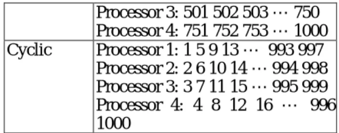
(4) 2.3. Loop Partitioning. If a loop can be executed in parallel, we want to break this loop down into a set of tasks on different processors. As we know, task granularity, which is an important issue in loop partitioning, heavily influences load balancing. Therefore, a good loop-partitioning algorithm will achieve better load balancing with only a small overhead. Currently, there are several loop-partitioning methods available in different loop scheduling algorithms, for example, SS, GSS, CSS, Factoring, and TSS [9, 10, 11, 12, 13, 14]. Assume that the number of processors available is P, the number of iterations of the DOALL loop is n, and the size of ith partition is Ki. Formulas for calculating Ki in different algorithms are listed in Table 1, where the CSS/k algorithm partitions the DOALL loop into k equal-sized chunks. Table 2 gives sample partition sizes for SS, CSS(125), CSS/4, GSS, Factoring, and TSS(88, 12) when N = 1000 and P = 4. Table 1. Margin specifications Scheme SS CSS(k) CSS/λ GSS Factoring TSS(f,l). Formulas Ki=1 Ki=k Ki=N/λ Ki=Ri/P,R0=N, Ri+1= Ri- Ki Ki=(1/2)┌i/P┐×N/P Ki=f – i ×δ, I=2N/(f+l), δ=(f-l)/(I-1) Table 2. Simple examples. Scheme SS CSS(125) CSS/4 GSS. N=1000 and P=4 1 1 1 1 1 1 1 1 1 1 1 1 1… 125 125 125 125 125 125 125 125 250 250 250 250 250 188 141 106 79 59 45 33 25 19 14 11 8 6 43321111 Factoring 125 125 125 125 62 62 62 62 32 32 32 32 16 16 16 16 8 8 8 8 4 4 4 4 2 2 2 2 1 1 1 1 TSS(88,12) 88 84 80 76 72 68 64 60…12. What we have mentioned above is dynamic loop partitioning. We must emphasize here that there are some differences between loop partitioning and loop scheduling. One partition has to be mapped to a processor; since there is no scheduler, we have to simulate a scheduler in generated programs. We will leave it as the future work. An alternative is static scheduling. The number of chunks equals the number of processors. There are two static loop scheduling methods: block and cyclic [15]. It is a tradeoff between locality and workload distribution. As method of block assigns a block of continuous iterations to one processor, method of cyclic assigns an amount of cyclic iterations to one processor. Simple examples are shown in Table 3. ADPPG implemented with static scheduling only, and the default is block scheduling. Table 3. Simple examples of block and cyclic scheduling Scheme Block. N=1000 and P=4 Processor 1: 1 2 3 4 5 6 7 … 250 Processor 2: 251 252 253 … 500.

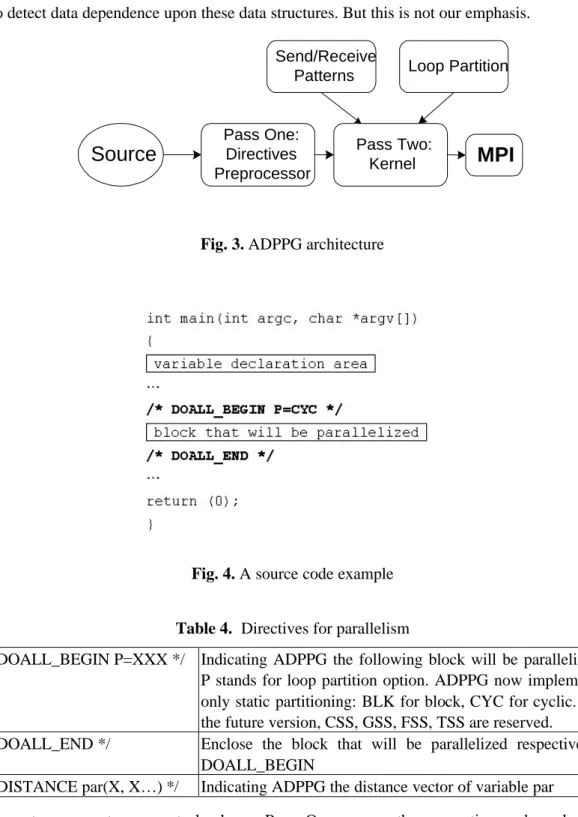
(5) Cyclic. Processor 3: 501 502 503 … 750 Processor 4: 751 752 753 … 1000 Processor 1: 1 5 9 13 … 993 997 Processor 2: 2 6 10 14 … 994 998 Processor 3: 3 7 11 15 … 995 999 Processor 4: 4 8 12 16 … 996 1000. 2.4. Communication Model. Communication model analysis is very important in translating sequential codes to parallel. Different models have different send/receive patterns. In [16], McGarvey et al. classified four categories of point update methodology: Independent, Nearest Neighbor, Quasi-Global and Global. The most we care is whether communication occurs among all processors. We simplify the classification into three types: Independent, Semi-Global, and Global as shown in Fig. 2.. Algorithm. Algorithm. Algorithm. (a) Independent. (b) Semi-Global. (c) Global. Fig. 2. Communication Models Each node (processor) executes some algorithms and depends on previous data. If the data required comes from itself, it is Independent. It commonly referred to as “embarrassingly parallel”, such as calculating the value of PI, Mandelbrot set, and matrix manipulations, etc. If the data comes from some of others, it is Semi-Global. This kind of communication model complicates the mapping from sequential to parallel, because we have to parse the semantics more precisely to get more information about passing messages to which nodes. So far we have few idea but some loop carried dependence distance directives about it. We will leave it as future efforts. Jacobi Iteration with data dependence distance vectors (-1, -1), (-1, 1), (1, -1) and (1, 1) belongs to this model. Otherwise, the data comes from all others and it is Global. One such communication model is all-pairs shortest path problem.. 3.. Design Approach. 3.1. System Model. ADPPG is an automatic directive-based code generator that translates a sequential source code to parallel one, as shown in Fig. 3. A source C program with directives, as example source code shown in Fig. 4, is fed to ADPPG. The directives we define are listed in Table 4. The source C program is not full version of C but a subset of it. Pointers and indirect array references are excluded for two reasons. First, it is not easy to parse these data structures. Second, it is difficult to implement sending.

(6) messages of these data types. So only subset of C is provided. As mentioned in other papers, it is not easy to detect data dependence upon these data structures. But this is not our emphasis. Send/Receive Patterns. Source. Pass One: Directives Preprocessor. Loop Partition. Pass Two: Kernel. MPI. Fig. 3. ADPPG architecture. Fig. 4. A source code example Table 4. Directives for parallelism /* DOALL_BEGIN P=XXX */ Indicating ADPPG the following block will be parallelized. P stands for loop partition option. ADPPG now implements only static partitioning: BLK for block, CYC for cyclic. For the future version, CSS, GSS, FSS, TSS are reserved. /* DOALL_END */ Enclose the block that will be parallelized respective to DOALL_BEGIN /* DISTANCE par(X, X… ) */ Indicating ADPPG the distance vector of variable par Our system uses two-pass technology. Pass One parses the semantics and analyzes the communication models of blocks enclosed with DOALL_BEGIN and DOALL_END directives. Pass Two mainly concentrates on loop parallelism and it will take loop-partitioning options into consideration. When parallelizing loops, Pass Two will take communication models analyzed by Pass One as information to map sequential behavior to send/receive patterns. After all, it will generate codes using C with MPI. We will discuss detail algorithms more clearly in the following..

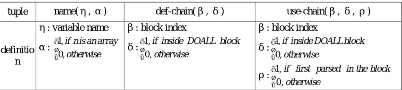
(7) 3.2. Pass One. Pass One will parse semantics of the program including distinguishing the master and slaves, parsing loop iterations, detecting message-passing behavior between two blocks and detecting communication models. Pass One is block oriented. The source program will be separated into several blocks according to DOALL loops. In other words, a DOALL loop is a breaking point. Each DOALL loop is a block, and each segment between two DOALL loops is also a block. Each block is indexed with an integer number starting with 1. The non-DOALL blocks excluding variable declaration parts only belong to the master. Other parts of the source program belong to both the master and slaves. The parts of the master will be enclosed with if (adppg_rank == 0) control flows with an error handling mechanism that ensures all processes exit at the same time. Iteration information of DOALL loops will be recorded and later used for loop partitioning. How many DOALL loops are there? What are the loop iteration variable name, lower bound and upper bound? All these will be recorded. To reduce synchronization, only the outer loop will be parallelized. The following structure is introduced to store loop iteration information. typedef struct{ char name[128]; char begin[128]; char end[128]; char step[128]; } ForIterator; If we have a statement: for (i=0; i<N; i=i+1), for example, we will record name=i, begin=0, end=N and step=1. The goal of recording iteration information is to calculate its space, and according to our record, the space is “N-0” which will be calculated in compile time (N is a constant) or run time (N is a variable). If the step is 1, it is block scheduling. Otherwise, it is cyclic scheduling. A def-use symbol table will be established for analyzing message-passing behavior. Each item in the table contains three fields: name tuple, def-chain tuple, use-chain tuple. The definition is described in Table 5. Table 5. Tuple used in def-use symbol table tuple. name(η, α) η: variable name 1, if n is an array. definitio α: 0, otherwise  n. def-chain(β, δ) β: block index 1, if inside DOALL block  0 , otherwise. δ: . use-chain(β, δ, ρ) β: block index 1, if inside DOALL block 0, otherwise. δ: . 1, if first parsed in the block  0 , otherwise. ρ: . To maintain the def-use symbol table, there are some rules: Given a variable η 1. if η is new to the table, create an item to the table, field of name tuple is (η, α) 2. if η is defined (write to η), add (β, δ) to def-chain field 3. if η is used (read from η) and ( (β, δ, ρ) or (β, δ, 0)) not in use-chain field, add (β, δ, 1).

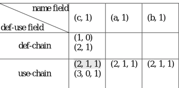
(8) For example, a source code is given and shown in Fig. 5. After parsing S1 to S6, the def-chain symbol table will be built as shown in Table 6. Iterations will not be added to the table since they are recorded in another data structure for further loop partitioning.. Fig. 5. Code segment of Matrix Multiplication Table 6. Def-use symbol table name field (c, 1). (a, 1). (b, 1). (2, 1, 1). (2, 1, 1). def-use field def-chain. (1, 0) (2, 1). use-chain. (2, 1, 1) (3, 0, 1). We will check the table for message-passing behavior and further communication models. If in the same block, there exists a use-chain tuple(β, δ, 1), it uses data in the previous block. In other words, sending data from previous block to current block is required. Followed is a detecting communication model. Assume a variable η is inside DOALL, if there exists no η is an array, the DOALL belongs to Independent. If there exists an array variable η, and there exists tuples of def-chain and use-chain of the same DOALL block, data exchange inside the DOALL may occur. Analysis of iteration dimension space should be taken. We do not unroll iteration space but dimension space ofη. The same technology of iteration space, if two nodes in the space have no relation between each other, it is message-independent. Otherwise, it is messagedependent. If there exists no message-independent, the DOALL belongs to Independent communication model. If some nodes, not all, in one dimension are message-dependent, the DOALL belongs to Semi-global. If all nodes are message-dependent in at least one dimension, the DOALL belongs to Global. Of the Global communication model, the message-dependent dimension determines the amount of message should be exchanged. Data only in the message-dependent dimension should be exchanged. If the DOALL is a nested-loop, the loop structure should be reconstructed. The loop controls the message-dependent dimension should be moved to be the outer loop. This approach is effective though easy to understand..

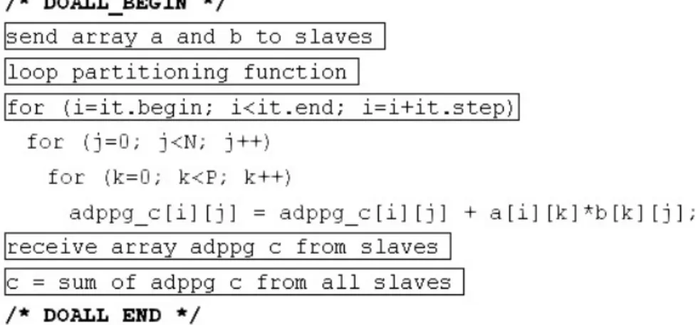
(9) 3.3. Pass Two. Pass Two mainly concentrates on DOALLs. The MPI function calls used in our system is listed in Table 7. We will take matrix multiplication shown in Fig. 5 as an example. Since there exist usechain tuple(β, δ, 1), two arrays (a and b) will be sent to slaves. Following is a loop partitioning function according to loop partitioning option. After that, we have to change the iteration control values in the following for statement. Different communications models have different send/receive patterns. The patterns will be taken into consideration to perform properly send/receive behavior. The code will be generated is shown in Fig. 6. Table 7. MPI function calls used Name MPI_Init MPI_Finalize MPI_Comm_rank MPI_Comm_size MPI_Send MPI_Recv MPI_Bcast. Functionality Start up MPI Shut down MPI Return the rank of calling process Return the size of communicator relative to calling process Send data to destination process Receive data sent by source process Send data to every process. Fig. 6. Matrix Multiplication after Pass Two. 4.. Experimental Results. 4.1. Our System Environment. Our SMPs cluster is a low cost Beowulf class supercomputer that utilizes a multi-computer architecture for parallel computations. The Parallel Testbed consists of two PC clusters. One is used for parallel computing, the other is used for high available application. For parallel computation portion, the snapshot of our cluster that consists of 8 PC-based symmetric multiprocessors (SMP) connected by two 24-port 100Mbps Ethernet SuperStackII 3300 XM switches with Fast Ethernet interface..

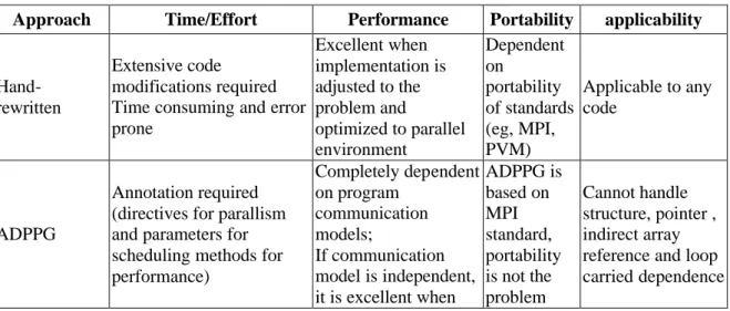
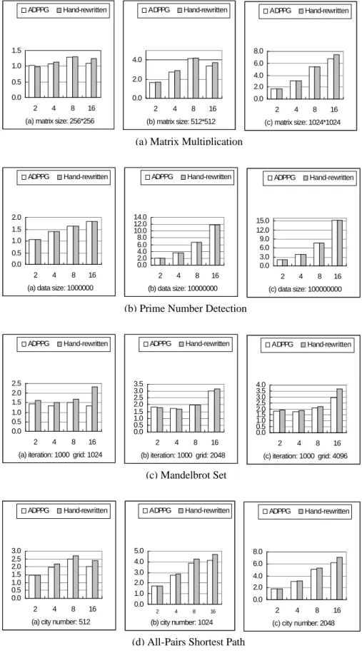
(10) There are one server node and fifteen computing nodes. The server node has two Intel Pentium-III 1GHz (FSB 133MHz) processors and 768MBytes of shared local memory. Each Pentium-III has 32K on-chip instruction and data caches (L1 cache), a 256K on-chip four-way second-level cache with full speed of CPU. Each P-III-based computing node with two 1G P-III processors has 512MBytes of shared local memory. We conduct four case studies as our experiments. 4.2. Experiments. Four study cases are considered to measure the correctness and performance. The first three study cases are: matrix multiplication, prime number detection, and mandelbrot set. They all belong to “Independent” communication model but behave a few different to each other. Since they are Independent, they do not have to communicate to each other while doing computation. The last study case is: all pairs shortest path. It belongs to “Global” communication model. Each processor has to use data from all other processors to update its own data. For each case, we have three versions of program: sequential, ADPPG generated, and hand-rewritten. Experiments are applied on various numbers of iteration with various numbers of processors. Finally the comparison between using our ADPPG and hand-rewritten is given. The execution time is shown in Table 9 and Table 10 followed by the speedup shown in Fig. 7. From the comparison of experimental results, hand-rewritten optimized codes perform more efficient than ADPPG generated codes. Analyzing codes of these different approaches, there are two main reasons cause the difference. First, the mechanism of handling errors of blocks belonging to master reduces the performance. Second, as we all know, collective communications have better performance than point-to-point ones. But in our ADPPG, it generates codes using point-to-point behavior. These will be taken into consideration for optimization of future ADPPG version. 4.3. Comparison. As shown in the above experimental results, we can have a comparison of our Automatic Directivebased Parallel Program Generator (ADPPG) and hand-rewritten optimized approach. The comparison is summarized in Table 8. Table 8. Comparison of ADPPG and hand-rewrittend approach Approach. Handrewritten. ADPPG. Time/Effort. Performance Excellent when Extensive code implementation is modifications required adjusted to the Time consuming and error problem and prone optimized to parallel environment Completely dependent on program Annotation required communication (directives for parallism and parameters for models; If communication scheduling methods for model is independent, performance) it is excellent when. Portability Dependent on portability of standards (eg, MPI, PVM) ADPPG is based on MPI standard, portability is not the problem. applicability. Applicable to any code. Cannot handle structure, pointer , indirect array reference and loop carried dependence.

(11) user tunes the code well. 5.. Conclusions and Future Work. We provide beginners a good learning tool to parallel programming with MPI. Users can use our system to generate parallel codes from sequential ones and can look closer to the relation between sequential and parallel codes. Moreover, they can also learn how to implement loop partitioning. Since the generated parallel codes’ performance are not much worse than the optimized codes, it is also a good tool to speedup the solving step or port current applications to parallel architectures with MPI implementation. One of our future works is to implement dynamic scheduling into our system, and the users will have more choices to tune generated codes to adjust their environments (homogeneous or heterogeneous). Another work is to use SUIF [17] to re-implement our system and using our technique of message-passing behavior analyzer to improve its loop transformation. Of course, the code optimization is the most important work in the near future. We will improve send/receive behavior for different communication models, and use the technology described in [18] to reconstruct point-to-point interaction to collective communication.. References [1] [2]. [3] [4] [5] [6] [7] [8] [9]. [10] [11] [12]. [13]. [14]. http://www.top500.org, TOP500 Supercomputer Sites. T. L. Sterling, J. Salmon, D. J. Backer, and D. F. Savarese, “How to Build a Beowulf: A Guide to the Implementation and Application of PC Clusters”, 2nd Printing, MIT Press, Cambridge, Massachusetts, USA, 1999. B. Wilkinson and M. Allen, “Parallel Programming: Techniques and Applications Using Networked Workstations and Parallel Computers”, Prentice Hall PTR, NJ, 1999. R. Buyya, High Performance Cluster Computing: System and Architectures, Vol. 1, Prentice Hall PTR, NJ, 1999. http://www.epm.ornl.gov/pvm/, PVM – Parallel Virtual Machine. http://www-unix.mcs.anl.gov/mpi/, The Message Passing Interface (MPI) standard http://www.lam-mpi.org, LAM/MPI Parallel Computing. M. Wolfe, “High-Performance Compilers for Parallel Computing”, Addison-Wesley Publishing, NY, 1996. C.T. Yang, S.S. Tseng, Y.W. Fan, T.K. Tsai, M.H. Hsieh, and C.T. Wu, “Using Knowledgebased Systems for research on portable parallelizing compilers,” Concurrency and Computation: Practice and Experience, vol. 13, pp. 181-208, 2001. S. F. Hummel, E. Schonberg and L. E. Flynn, “Factoring: A method for scheduling parallel loops,” Communication of ACM, Vol. 35, No. 8, 1992, pp. 90-101. C. P. Kruskal and A. Weiss, “Allocating independent subtasks on parallel processors”, IEEE Transactions on Software Engineering, Vol. 11, No. 10, 1985, pp. 1001-1016. C. D. Polychronopoulos and D. J. Kuck, “Guided self-scheduling: A practical self-scheduling scheme for parallel supercomputers”, IEEE Transactions on Computer, Vol. 36, No. 12, 1987, pp. 1425-1439. T. H. Tzen and L. M. Ni, “Trapezoid self-scheduling: A practical scheduling scheme for parallel compilers”, IEEE Transactions on Parallel Distributed Systems, Vol. 4, No. 1, 1993, pp. 87-98. P. Tang and P. C. Yew, “Processor self-scheduling for multiple-nested parallel loops”, in Proceedings of the 1986 International Conference on Parallel Processing 1986, pp. 528-535..

(12) [15] H. Li, S. Tandri, M. Stumm and K. C. Sevcik, “Locality and loop scheduling on NUMA multiprocessors”, in Proceedings of the 1993 International Conference on Parallel Processing, Vol. II, 1993, pp. 140-147. [16] B. McGarvey, R. Cicconetti, N. Bushyager,E. Dalton, “Beowulf Cluster Design for Scientific PDE Models”, http://www.athena-em.atech.edu/Beowulf/index.html [17] http://suif.stanford.edu, The Stanford SUIF Compiler Group. [18] Beniamino Di Martinoa, Antonino Mazzeob, Nicola Mazzoccaa,Umberto Villanoc, “Parallel program analysis and restructuring by detection of point-to-point interaction patterns and their transformation into collective communication constructs”, Science of Computer Programming, vol. 40, pp.235-263, 2001..

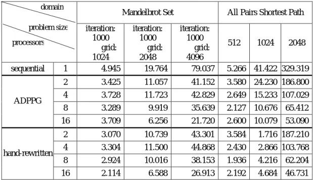
(13) Table 9. Execution time of Matrix Multiplication and Prime Number Detection domain. Matrix Multiplication. Prime Number Detection. problem size. 256*256. processors. sequential. ADPPG. hand-rewritten. 512*512 1024*1024 1000000 10000000 100000000. 1. 1.494. 20.819. 170.530. 1.178. 29.566. 780.085. 2. 1.456. 13.088. 102.410. 1.128. 15.552. 393.220. 4. 1.382. 7.616. 55.337. 0.845. 8.258. 202.569. 8. 1.166. 4.989. 31.490. 0.719. 4.407. 101.564. 16. 1.355. 6.223. 25.161. 0.646. 2.508. 51.096. 2. 1.515. 12.136. 101.545. 1.128. 15.619. 393.854. 4. 1.326. 7.265. 56.811. 0.837. 8.273. 202.532. 8. 1.136. 4.893. 31.352. 0.724. 4.405. 101.579. 16. 1.195. 5.596. 22.891. 0.645. 2.508. 51.086. Table 10. Execution time of Mandebrot Set and All Pairs Shortest Path domain problem size. ADPPG. hand-rewritten. All Pairs Shortest Path. 1. iteration: 1000 grid: 1024 4.945. iteration: 1000 grid: 2048 19.764. iteration: 1000 grid: 4096 79.037. 5.266 41.422 329.319. 2. 3.425. 11.057. 41.152. 3.580 24.230 186.800. 4. 3.728. 11.723. 42.829. 2.649 15.233 107.029. 8. 3.289. 9.919. 35.639. 2.127 10.676. 65.412. 16. 3.709. 6.256. 21.720. 2.600 10.079. 53.090. 2. 3.070. 10.739. 43.301. 3.584. 1.716 187.210. 4. 3.304. 11.500. 44.868. 2.430. 2.866 103.768. 8. 2.924. 10.016. 38.153. 1.936. 4.216. 62.204. 16. 2.114. 6.588. 26.913. 2.192. 4.684. 46.731. processors. sequential. Mandelbrot Set. 512. 1024. 2048.

(14) ADPPG. Hand-rewritten. ADPPG. Hand-rewritten. 1.5. ADPPG. Hand-rewritten. 8.0 4.0. 1.0 0.5. 2.0. 0.0. 0.0. 6.0 4.0 2.0. 2. 4. 8. 0.0. 16. 2. (a) matrix size: 256*256. 4. 8. 16. 2. (b) matrix size: 512*512. 4. 8. 16. (c) matrix size: 1024*1024. (a) Matrix Multiplication ADPPG. Hand-rewritten. ADPPG. Hand-rewritten. ADPPG. 14.0 12.0 10.0 8.0 6.0 4.0 2.0 0.0. 2.0 1.5 1.0 0.5 0.0 2. 4. 8. 16. 15.0 12.0 9.0 6.0 3.0 0.0 2. (a) data size: 1000000. Hand-rewritten. 4. 8. 16. 2. (b) data size: 10000000. 4. 8. 16. (c) data size: 100000000. (b) Prime Number Detection ADPPG. Hand-rewritten. 2.5 2.0 1.5 1.0 0.5 0.0. ADPPG. Hand-rewritten. ADPPG. 3.5 3.0 2.5 2.0 1.5 1.0 0.5 0.0. 2. 4. 8. 16. 4.0 3.5 3.0 2.5 2.0 1.5 1.0 0.5 0.0 2. (a) iteration: 1000 grid: 1024. Hand-rewritten. 4. 8. 16. 2. (b) iteration: 1000 grid: 2048. 4. 8. 16. (c) iteration: 1000 grid: 4096. (c) Mandelbrot Set ADPPG. Hand-rewritten. 3.0 2.5 2.0 1.5 1.0 0.5 0.0 2. 4. 8. 16. (a) city number: 512. ADPPG. Hand-rewritten. 5.0 4.0 3.0 2.0 1.0 0.0. ADPPG. Hand-rewritten. 8.0 6.0 4.0 2.0 0.0 2. 4. 8. 16. (b) city number: 1024. (d) All-Pairs Shortest Path. Fig. 7. Speedup of case studies. 2. 4. 8. 16. (c) city number: 2048.

(15)