Multi-class named entities extraction from biomedical literature

Multi-class Named Entities Extraction

from Biomedical Literature

*

TYNE LIANG AND JIAN-SHIN CHEN Institute of Computer and Information Science

National Chiao Tung University Hsinchu, 300 Taiwan

With rapid growth of electronic literature in recent years, efficient named entities extraction becomes an indispensable part of knowledge base construction automation. In this paper an entity extraction system useful as biomedical knowledge acquisition was presented. Unlike most entity extraction systems which do not concern term variants, the proposed system was incorporated with a rule-based resolver to recover the full forms of those target entities from the coordination variants. The resolution approach was proved with GENIA Corpus 3.0 to be feasible by showing 88.51% recall and 57.04% precision. On the other hand, the kernel part of the system was based on Hidden Markov Model (HMMs) by setting appropriate set of input features extracted from training corpus. With various experiments on different corpora the proposed system achieved promising results at entity boundary identification and at classification as well.

Keywords: named entity extraction, biomedical literature, statistical model, term variant, classification

1. INTRODUCTION

With the explosive growth of biomedical research, huge amounts of biomedical lit-erature are produced. For instance, the number of PubMed citations increases nearly 69% in recent ten years [1]. Therefore efficient information extraction (IE) systems are needed to facilitate biomedical knowledge bases construction and maintenance as well [2]. One fundamental task involved with the IE process is identification and classification of biomedical entities. Nevertheless, such tasks in biomedical domains become more complicated due to open vocabulary, irregularity of naming, semantic crossover and boundary identification. For example, the number of entries in Swiss-Prot version 42.0 [3], a protein knowledge base, increases 277.36% in recent ten years. Out of 135,850 entries, each entry contains 2.54 synonyms in average, and each synonym contains 2.74 words in average.

In recent literature, named entity extraction by using rule-based, statistical or hybrid approaches, have been proposed. Rule-based approaches concern the nomenclature of named entities. Two famous rule-based identifiers were developed, namely, KeX [4] and Yapex [5], for protein entities extraction only. Yet rule-based methods are essentially lack of portability and scalability.

Statistical methods have been presented by applying different models like Hidden

Received July 7, 2004; revised November 12, 2004 & August 12, 2005; accepted November 17, 2005. Communicated by Suh-Yin Lee.

Markov Model (HMM), Maximum Estimation (ME), Support Vector Machine (SVM), Naïve Bayes (NB) … etc [6-11]. The recognition accuracy achieved by these models generally depends on a well-tagged training corpus and well set of input features [8, 11, 14]. Well-known training corpus like GENIA 3.01 [12] has been widely used for training models. As to feature selection, Kazama et al. [8] found that Left Word Cache, Right Word Cache, Right Word Cache, Preceding Class and Suffix play positive effect. Lee et al. [11] indicated that features have different contribution in different phases. At identi-fication phase Word, POS, Suffix and Prefix are positive features; while predefined Func-tional Words, Word List, Nouns, and Verbs are useful at classification phase. On the other hand, Zhou et al. [14] showed that POS is very useful in biomedical domain with the increase of 22.6 F-score while special verbs turn out to be negative feature. Other feathers like conditional random fields (CRF) are introduced in [20] and are reported to be helpful to enhance recognition accuracy with the implementation of an HMM-based recognition model.

Some hybrid approaches were proposed by using coded rules, statistical model and outer resources like dictionaries. For example, Proux et al. [13] built a system to detect gene symbols and names in biological texts. The backbone of the system is a tagger for tokenization, lexical lookup, and disambiguation. To deal with unknown words, it used lexical rules to obtain candidates and used a HMM-based disambiguator for further veri-fication. On the other hand, Zhou et al. [14] exploits a very rich set of features on their HMM-based PowerBioNE in which a k-NN algorithm is used for tackling sparseness and a pattern-based post-processing is embedded to handle abbreviation and cascaded entity name phenomenon in GENIA 3.0 corpus. Without the help of dictionary the system out-performs some statistical approaches by achieving the F-measure of 66.6 and 62.2 on 23 classes of GENIA V3.0 and V1.1 respectively.

In fact, entity recognition involves identification and classification. In [15] identifi-cation of a single class was done in such a way that candidate entities were validated with a scoring method. The finding of candidate entities can be done by lexical rules, rule-based segmentation approach, or approximate string searching with a help of dic-tionary. Subsequent verification of candidates can be done by statistical models like HMM, and NB. Some systems assume the identification task is done and well, so they focused on classification only and usually yielded better results [16].

In this paper, an on-line corpus-based extractor useful for extracting multi-class biomedical entities was presented. Unlike most of previous researches in named entity extraction, the presented extractor was embedded with a term variant resolver for recov-ering those target entities expressed in coordination variants which are common phe-nomenon in written texts. The resolver was built by applying a set of heuristic rules to-gether with clustering strategies to boost recognition precision. Experimental results on GENIA corpus proved the feasibility of the proposed approach by achieving 88.51% recall and 57.04% precision.

On the other hand, the kernel part of the presented extractor is based on a simple HMM-based model since such learning approach becomes widely explored with the availability of a tagged corpus like GENIA 3.0. However GENIA 3.0 is an unbalanced for its twenty-three different entity classes. For example there are more than 19000 in-stances for class “protein-substructure” while only 2 and 88 inin-stances are for classes “or-ganic” and “carbohydrate” respectively. In order to include more instances of target

enti-ties for the proposed HMM-based extractor, we classified all entienti-ties into four classes rather than 23 classes in accordance to GENIA ontology. The classes are “protein”, “DNA/RNA”, “source”, and “other biomedical entities” (“Other-Bio” for short).

The presented extractor was implemented for entity identification and classification in such a way that 90% of the GENIA 3.01 corpus was used as training data and the re-maining 10% for system testing. On 1,685 testing sentences, the proposed system achieved promising results by showing 72% recall and 66% precision at boundary identi-fication and 63% recall and 57% precision for four target entity types. Such results are encouraging for three reasons. First, the extractor was built up without any predefined patterns or the help of outer dictionaries. Second, unlike other extractors which generally exploit a rich set of features, the presented HMM-based extractor is constructed by using POS feature only. So it has less cost at extraction time and space overhead. Third, the target entities to be recognized are those with the largest annotation and the target entity boundaries identification is evaluated with strict annotation, so higher F-score can be expected if flexible annotation, as defined in [5], is made.

The remaining part of this paper is organized as follows. Section 2 describes the corpus and the target named entities. Section 3 explains our document preprocessing and feature extraction. Section 4 presents the coordination variants resolver and the corre-sponding verification. Similarly section 5 describes the HMM-based named entity ex-tractor and its comparisons to other approaches in terms of various measurements. Fi-nally, section 6 makes the conclusion and future works.

2. THE CORPUS AND THE TARGET NAMED ENTITIES

The corpus we used in this paper is GENIA version 3.01 which contains 1999 (one duplicate is removed) Medline abstracts and it is encoded in GENIA Project Markup Language (GPML). In GENIA corpus, biomedical terms are defined according to the terminal concepts in GENIA ontology. The annotated named entity can be divided into five types according to their coverage of boundaries. They are: simple annotated named entity, recursively annotated named entity, simple annotated coordination variants, recur-sively annotated coordination variants, and incomplete named entity.

Simple annotated named entities, like “primary T lymphocytes” marked as <cons sem=“G#cell_type”> primary T lymphocytes </cons>, are the main part in GENIA cor-pus. Recursively annotated named entities are represented in a nested form. One narrow concept is covered by another broader concept. For example “IL-2 gene” indicates a DNA domain or region, but term “IL-2 gene expression” becomes the functional entity in the sentence.In [14], Zhou et al. tackled such cascaded entity name phenomenon with a pattern-based post-processing.

Simple annotated coordination variants are one of common writing phenomena. For example, “CD8+ and CD4+ cells” implies “CD8+ cells and CD4+ cells”. Recursively annotated coordination variants is like “B and T lymphocyte activation and mitogenesis” which can be expanded into four independent entities, namely, “B lymphocyte activa-tion”, “B lymphocyte mitogenesis”, “T lymphocyte activaactiva-tion”, and “T lymphocyte mi-togenesis”. GENIA corpus marked this kind of named entity using a nested boundary, like <cons sem=“(AND (AND G#other_name G#other_name) (AND G#other_name G#other_name))”>.

In a coordinated variant, parts of the named entities are omitted and the remaining parts becoming incomplete terms. GENIA annotates these kinds of incomplete terms with a non-semantic tag <cons> … </cons>, indicating the concept in the chunk unde-fined. For example “CD8+”, “CD4+” and “B” and “T” in the above examples are incom-plete terms if they appear alone.

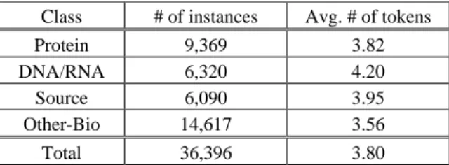
In this paper, the target entities are classified into four types rather than 23 types. This is because, first, GENIA 3.0 is an unbalanced corpus for 23 classes of biomedical entities and second, only those entities with largest boundaries will be treated as target entities. So we have less number of entities in GENIA 3.0. For example, “IL-2 gene ex-pression” will be treated as one single entity tagged with “other-name” rather than two entities: “IL-2 gene” (tagged with “DNA-domain-or-region”) and “IL-2 gene expression” (tagged with “other-name”). In fact, such handling is correct for named entities extrac-tion in system realizaextrac-tion. In order to increase more instances of training data, we clas-sify entities into four major classes in order to increase more instances of training data. Table 1 indicates the mapping between the four major concepts (namely, Protein, DNA/RNA, Source, and Other-Bio) and their corresponding concepts in GENIA corpus. Table 2 shows the statistics of the target entity instances.

Table 1. The target named entities in terms of GENIA ontology.

Class Semantic

Protein

amino acid, protein, protein molecule, protein family or group, protein domain or region, protein structure, protein complex, protein N/A, peptide, amino acid monomer

DNA/RNA

DNA molecule, DNA family or group, DNA domain or region, DNA substruc-ture, DNA N/A, RNA molecule, RNA family or group, RNA domain or region, RNA substructure, RNA N/A, polynucleotide, nucleotide

Source multi cell, mono cell, virus, body part, tissue, cell type, cell line, other artificial source

Other-Bio organic, lipid, carbohydrate, other organic compound, inorganic, atom

Table 2. Statistics of entity instances per entity class. Class # of instances Avg. # of tokens

Protein 9,369 3.82

DNA/RNA 6,320 4.20

Source 6,090 3.95

Other-Bio 14,617 3.56

Total 36,396 3.80

As shown in Table 2, a biomedical named entity in our training corpus is composed of 3.8 tokens in average. So correct boundary identification of a named entity will en-hance correct entity classification. To deal with boundary identification, we used BIO representation for entity recognition. The boundary information is represented as the

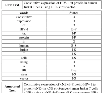
class prefixes “B-”, “I-”, and “O”, indicating the current word at the “beginning of”, “in”, “not” word of a named-entity. If there are n classes of named entities to be identified, the BIO representation will yield 2n + 1 states. Table 3 shows the corresponding states of an example sentence.

Table 3. Example of a target sentence and its corresponding BIO-states.

Raw Text Constitutive expression of HIV-1 tat protein in human

Jurkat T cells using a BK virus vector.

words States Constitutive O expression O of O HIV-1 B-P tat I-P protein I-P in O human B-S Jurkat I-S T I-S cells I-S using O a O BK B-S virus I-S vector I-S Annotated Text

Constitutive expression of <NE cl=Protein>HIV-1 tat protein</NE> in <NE cl=Source>human Jurkat T cells </NE> using a <NE cl=Source>BK virus vector</NE>.

3. CORPUS PROCESSING AND FEATURE EXTRACTION

In the corpus processing, we used two available natural language processing tools: SentenceSplitter [17] and MINIPAR [18] for sentence segmentation and parsing. Then different types of features, including internal, external and global features, were stored for model comparison. Internal features are orthographical features (such as capital letter, numerical number, … etc) and morphological features (such as prefix and suffix). Exter-nal features concern the role that a word plays in a sentence, for example a word’s POS. With the help of MINIPAR, there are twenty-one POS features used as the external fea-tures. The global features are the lexicons with top-20 chi-square values per target entity class. They are mined from the training corpus.

4. COORDINATION VARIANT RESOLUTION

Unlike most entity extractors which do not cope with term variants, the presented extractor was embedded with a coordination variant resolver to recover the full forms of

those entities in variants. In GENIA 3.01 corpus, there are 1598 coordination variants, covering 8.06% of corpus sentences and each variant contains 2.1 entities in average.

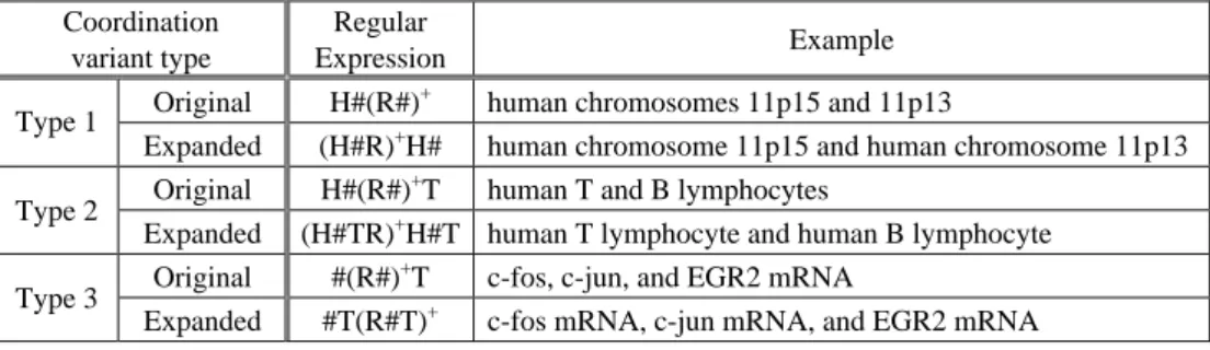
Table 4 lists the three common patterns summarized from GENIA corpus. In this table, “#” indicates the existing part of the un-recovered entity; “H” and “T”, denoted as head and tail terms respectively, are the words appearing in front and back of named en-tities respectively; “R” indicates conjunctive words in the coordination variants. In the training corpus 90.53% coordination variants are type-3 patterns, and 98.68% are the variants with “and”, “or”, and “but not”.

Table 4. Coordination variant patterns, expanded patterns and examples. Coordination

variant type

Regular

Expression Example Original H#(R#)+ human chromosomes 11p15 and 11p13 Type 1

Expanded (H#R)+H# human chromosome 11p15 and human chromosome 11p13 Original H#(R#)+T human T and B lymphocytes

Type 2

Expanded (H#TR)+H#T human T lymphocyte and human B lymphocyte Original #(R#)+T c-fos, c-jun, and EGR2 mRNA

Type 3

Expanded #T(R#T)+ _{c-fos mRNA, c-jun mRNA, and EGR2 mRNA}

Input: target sentence

target_word := first word of the target sentence.

while not (target_word = = the last word of the target sentence) do

success := pattern_identifier(target_word)

if success then

pattern_expander(target_word)

else

target_word := next word

end if end while

Fig. 1. Algorithm of coordination variant pattern handler.

The identification for variant types is implemented with finite state machines (FSM) which accept each word in the target sentence as the state transition entity and stop at the terminated state or till the end of the target sentence. Fig. 1 is the algorithm for identify-ing and expandidentify-ing variants. Procedure type_identifier() corresponds to the three-type FSMs. The algorithm ran three times for each of the three FSMs to check whether the target sentence contains any one of the three types patterns. The procedure pattern_ expander() will be executed for pattern expansion.

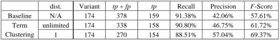
The performance of the handler is verified by a set of 1850 sentences in which 165 sentences contain 174 variant patterns. Experimental results showed that this approach yielded 91.38% recall and 42.06% precision (indicated as “baseline approach” in Table 5). To increase precision, we can design one FSM for each kind of sentence patterns, yet it will slow down the resolving throughput. For example a more complicated FSM is

Table 5. Accuracy of coordination variants identification on GENIA 3.01. dist. Variant tp + fp tp Recall Precision F-Score Baseline N/A 174 378 159 91.38% 42.06% 57.61% unlimited 174 338 158 90.80% 46.75% 61.72% Term

Clustering 1 174 270 154 88.51% 57.04% 69.37%

needed to handle a nested pattern like “B and T lymphocyte activation and mitogenesis”. Similarly a particular FSM is needed to resolve the examples like “IFN(gamma)” in “IFN(beta) and gamma”.

In order to increase the sensitivity of the pattern identifier, a simple term clustering which considers co-occurring terms, was applied. Let (ti, tj) co-occur in coordination variant, and (ti, tk) co-occur in another one. Then we put ti, tj and tk into one cluster. With term clustering strategy (indicated as “unlimited-distance” in Table 5), the recall and the precision become 90.8% and 46.75% respectively, increasing 4% F-Score. This shows that the clustering results become helpful to restrict the path movement in FSMs. To dis-tinguish the closeness of the terms in the same cluster, we furthermore applied the Floyd- Warshall algorithm in cluster sets. That is, if (ti, tj) co-occur in a phrase and (ti, tk) co- occur in another one but not (tj, tk), then the dist(tj, tk) = 2. With this clustering strategy, the precision became 57.04% (increasing 15% with respect to the baseline method) at the expense of lower recall. Table 5 shows that we can get the best result when the distance is equal to one. If we relax distance threshold, it can resolve more instances but most of them are false-positive instances.

5. HMM-BASED NAMED ENTITY EXTRACTOR

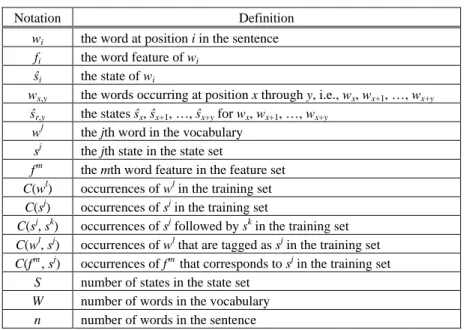
In Marcov-model tagging, the sequence of state tags in a sentence is regarded as a Marcov chain. Table 6 lists the notation used in Markov models. To learn the regularities of the state sequences, we used the tagged GENIA corpus 3.01 and construct the HMM- based entity extractor with the relative frequencies of words and the corresponding word features P(<wi, fi>|ŝi) rather than P(wi |ŝi) associated with traditional HMMs in which no word’s features are exploited. Then the optimal state assignment can be estimated by applying Bayesian rule and Markov assumptions (the limited horizon and time invariant) as Eq. (1). P(w1,n |ŝ1,n)P(ŝ1,n) = 1 [ (< , > n i i i P w f =

∏

|ŝi) × P(ŝi |ŝi-1)] (1) However many words in sentences we are going to tag are not in the training corpus. For example there are 4.25% (= 2028/47710) of words of our testing GENIA corpus are unknown words. Therefore we assume that the unknown words can be given a distribu-tion over the state quantity corresponding to that of the training corpus. But this ap-proach greatly disregards the lexical and contextual information, probably making accu-racy lower. Hence we use the internal features extracted from words and their contextual

Table 6. Notation used in Markov models. Notation Definition

wi the word at position i in the sentence

fi the word feature of wi

ŝi the state of wi

wx,y the words occurring at position x through y, i.e., wx, wx+1, …, wx+y

ŝr,y the states ŝx, ŝx+1, …, ŝx+y for wx, wx+1, …, wx+y

wl the jth word in the vocabulary sj the jth state in the state set

fm the mth word feature in the feature set

C(wl) occurrences of wl in the training set

C(sj) occurrences of sj in the training set

C(sj, sk) occurrences of sj followed by sk in the training set

C(wl, sj) occurrences of wl that are tagged as sj in the training set

C(fm, sj) occurrences of fm that corresponds to sj in the training set

S number of states in the state set

W number of words in the vocabulary

n number of words in the sentence

information like word dependency to make inference about an unknown word’s possible state. The distribution of word features involves reforming the word generation probabil-ity:

P(wl |sj) = P(f1 |sj)λ1× P(f2 |sj)λ2× … × P(fm |sj)λm. (2) Here λi = 1 or 0 depending on whether feature fi is used for unknown word identification or not. Thus the optimal states ŝ1,n of a word sequence can be determined by combining Eqs. (1) and (2) to be Eq. (3):

P(w1,n |ŝ1,n)P(ŝ1,n) = 1 { (< , > n i i i P w f =

∏

|ŝi)λ0× 1 [ ( m j j P f =

∏

|ŝi)λj] × P(ŝi | ŝi-1)}. (3) Here λ0 = 0 or 1 depending on whether the word is an unknown word or not. Then we have to find the following training data set:

P(sk |sj) = ( , ) ( ) j k j C s s C s (4) P(<wl, fim>|sj) = (< , >, ) , ( ) l m j i j C w f s C s ∀fi∈ F (5) P(fim |sj) = ( | ) , ( ) m j i j C f s C s ∀fi∈ F. (6)

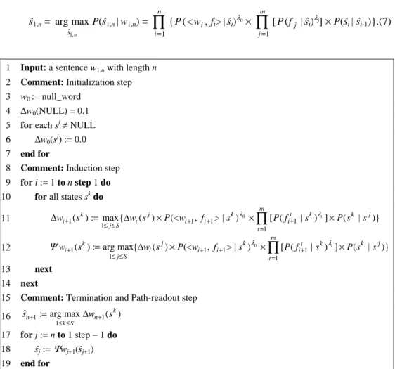
On the other hand, the tagging process at testing phase was implemented with Viterbi procedure in which function ∆wi(sj) yields the probability of being in state j at

word i and function Ψwi+1(sj) yields the most likely state at word i given that we are in

state j at word i + 1. We assume that there are “null words” in front of each sentence. The “null word” is always assigned with state NULL and with probability value 1.0 to the state NULL at initialization.

We construct Visible Markov Models in training but treat them as Hidden Markov Models when we use it to tag new corpora. This is because we can observe the states of the annotated corpus in training. The algorithm for tagging the states with visible Markov model tagger is showed in Fig. 2 in which the optimal states of a testing sequence are as the following equation:

ŝ1,n = 1, ˆ arg max n s P(ŝ1,n |w1,n) = 1 { (< , n i i P w =

∏

fi>|ŝi)λ0× 1 [ ( m j j P f =

∏

|ŝi)λj] × P(ŝi | ŝi-1)}.(7) 1 Input: a sentence w1,n with length n

2 Comment: Initialization step 3 w0 := null_word

4 ∆w0(NULL) = 0.1 5 for each sj≠ NULL 6 ∆w0(sj) := 0.0 7 end for

8 Comment: Induction step 9 for i := 1 to n step 1 do 10 for all states sk do

11 0 1 1 1 1 1 ₁ ( ) : max{ ( ) (< , > | ) [ ( | ) ]t ( | )} m k j k t k k j i i i i i j S _t w₊ s w s P w₊ f₊ s λ P f₊ s λ P s s ≤ ≤ ₌ ∆ = ∆ × ×

∏

× 12 0 1 1 1 1 1 ₁ ( ) : arg max{ ( ) (< , > | ) [ ( | ) ]t ( | )} m k j k t k k j i i i i i j S _t w s w s P w f s λ P f s λ P s s Ψ + + + + ≤ ≤ = = ∆ × ×

∏

× 13 next 14 next

15 Comment: Termination and Path-readout step

16 1 1 1 ˆn : arg max n ( k) k S s₊ w₊ s ≤ ≤ = ∆ 17 for j := n to 1 step − 1 do 18 ŝj := Ψwj+1(ŝj+1) 19 end for

Fig. 2. Algorithm for tagging states by the presented HMM-extractor.

5.1 Recognition Results and Analysis

(denoted as P), and f-score (defined as 2PR/(R + P)). R is calculated as tp/(tp + fn) and P is tp/(tp + fp) where ‘tp’ means true positive, ‘fn’ means false negative, and ‘fp’ means false positive. Since the proposed entity extractor can be tuned by feature selection, we defined F1 as the feature set in Eq. (5) for dealing with words in vocabulary, and F2 as

the feature set in Eq. (6) for dealing with the unknown words. The feature sets F1 and F2

are used as fi and fj in the Eq. (7) for the kernel function. Table 7 shows the best

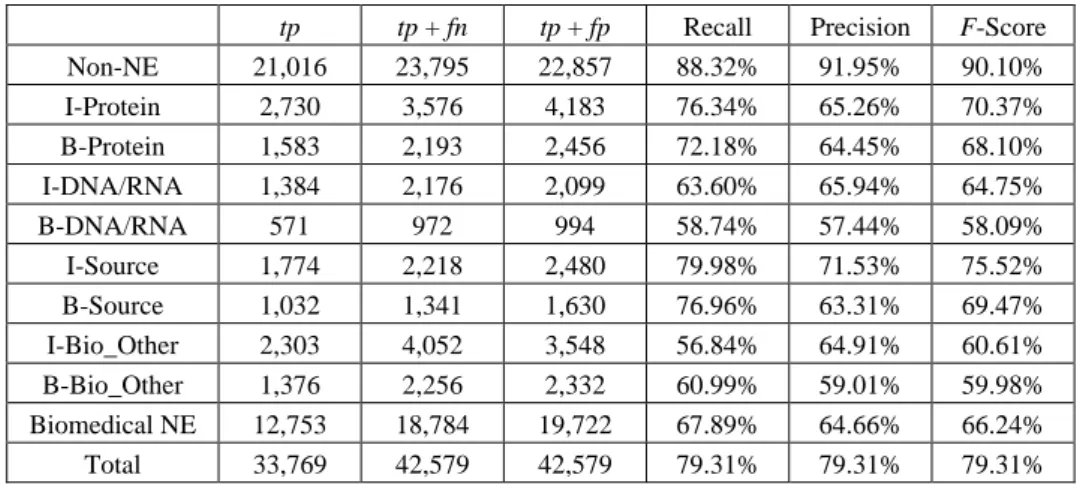
experi-ment results of entity boundary identification and entity classification by using POS fea-ture set only. This is because many biomedical entities are descriptive and very long [14]. For example, the protein entities in our experiments contain 3.8 words in average; 83.2% and 83.5% POS tags are “NN” on the first token and the last token respectively. It is also noticed, from Table 7, that lower accuracy was obtained for classes “DNA/RNA” and “Other-Bio”. The reasons for these results are less positive instances for “DNA/RNA” and wide varieties of entity types for “Other-Bio” in the corpus. Low classification also results from our evaluation by strict annotation. That means, the boundaries of target entities (with the longest boundaries in GENIA corpus) have to be completely matched with the annotations. However, if we relax strict annotation, higher classification accu-racy can be expected from the detailed classification results listed in Table 8.

Table 7. Named entity identification and classification with F1 = {Part-of-speech} and F2

= {Part-of-speech}.

tp tp + fn tp + fp recall precision F-score

Identification 4,855 6,762 7,412 71.80% 65.50% 68.51% Classification 4,235 6,762 7,412 62.63% 57.14% 59.76% Protein 1,476 2,193 2,456 67.31% 60.10% 63.50% DNA/RNA 536 972 994 55.14% 53.92% 54.53% Source 930 1,341 1,630 69.35% 57.06% 62.61% Other-Bio 1,293 2,256 2,332 57.31% 55.45% 56.36%

Table 8. Named entity classification with F1 = {Part-of-speech} and F2 = {Part-of-speech}.

tp tp + fn tp + fp Recall Precision F-Score

Non-NE 21,016 23,795 22,857 88.32% 91.95% 90.10% I-Protein 2,730 3,576 4,183 76.34% 65.26% 70.37% B-Protein 1,583 2,193 2,456 72.18% 64.45% 68.10% I-DNA/RNA 1,384 2,176 2,099 63.60% 65.94% 64.75% B-DNA/RNA 571 972 994 58.74% 57.44% 58.09% I-Source 1,774 2,218 2,480 79.98% 71.53% 75.52% B-Source 1,032 1,341 1,630 76.96% 63.31% 69.47% I-Bio_Other 2,303 4,052 3,548 56.84% 64.91% 60.61% B-Bio_Other 1,376 2,256 2,332 60.99% 59.01% 59.98% Biomedical NE 12,753 18,784 19,722 67.89% 64.66% 66.24% Total 33,769 42,579 42,579 79.31% 79.31% 79.31%

Other features like prefix or suffix features are not helpful due to their even distri-bution in target entity classes and non-entity classes, thus making them carry less dis-crimination. As to the global features like clue words mined from corpus by chi-square test, we found that the words with high values may make the state transition probability of the extractor not conspicuous. For instance, clue word “protein” is one of the mined lexicons in top-20 feature value in all the four target classes, thus slightly decrease over-all performances. However it might be still worthwhile to use some informative head-words at post-processing of classification for individual entity classes. For instance, “gene” for tagging “hematopoietic gene” with “DNA/RNA-class” and “cell” for tagging “hematopoietic gene cell” with “cell-class”.

Moreover, it is usual the case for biomedical named entity to be generated on the behavior of its source, which induces the problem of crossover between classes. For ex-ample “human NF-kappa B” should be chunked together as: “<cons sem=“G#protein_ molecule”>human<cons sem=“G#protein_molecule”>NF-kappa B</cons></cons>”. But we chunk it as “<NE cl=Source>human</NE> <NE cl=Protein>NF-kappa B</NE>”. Even though such tagging result is acceptable, we still treated it as wrong answer. In ad-dition, there exists some annotation inconsistency in GENIA corpus. As indicated in [14], it is expected to improve the extraction results through refinement of the annotation scheme in GENIA 3.0, such as flexible annotation scheme and annotation consistency and inclusion of an appropriate biomedical dictionary.

5.2 Recognition Model Comparison

The proposed system was compared to other statistical approaches and it was proved to be competitive in the same settings. The comparisons with other HMM-based approaches are made in terms of space and time complexity, identification and classifica-tion accuracy. The tradiclassifica-tional HMM approach (denoted as tradiclassifica-tional-tagger) was treated as baseline model and was compared with the presented HMM-based tagger (denoted as

presented-tagger) and the one proposed by Collier et al. (denoted as Collier-tagger) [6].

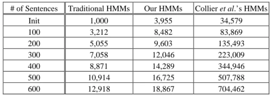
Essentially the time complexity of HMM-based tagger is O(n × S2), where n is the num-ber of words in the target sentence and S is the size of state set. The major factor that affects the performance of HMM-based tagger becomes the size of the state transition probability set. The larger the size of training probability set, the more time it will take on searching the corresponding probability of words, features, and states. Therefore it is noticed that when W is the size of vocabulary, F is the size of feature set, and S is the number of states, the space complexity for traditional-tagger and the presented-tagger become O(S2 + WS) ≈ O(WS) and O(S2 + WFS + FS) ≈ O(WFS) respectively. On the other hand, the space complexity of Collier-tagger becomes O(W2F2S2 + 2WF2S2 + F2S2

+ S2 + S) ≈ O(W2F2S2)

The three HMM-based taggers were trained with the same training data set (ran-domly selected 90% of GENIA ver. 3.01) and estimated by the same testing data set (re-maining 10% of GENIA ver. 3.01). All the three systems ran on the same platform, and used the same database.

For fair comparison, both Collier-tagger and the presented-tagger used the same features and for Collier-tagger the parameters were set to be λ0 = 0.9, λ1 = 0.04, λ2 = 0.04,

λ3 = 0.014, λ4 = 0.005, and λ5 = 0.001. All the three taggers were implemented with 100

testing sentences. Table 9 shows the execution time comparison result. The bigger the size of state transition probability set, the more time is spent for finding needed state transition probability.

Table 9. Execution time comparison. (Unit: msec)

# of Sentences Traditional HMMs Our HMMs Collier et al.’s HMMs

Init 1,000 3,955 34,579 100 3,212 8,482 83,869 200 5,055 9,603 135,493 300 7,058 12,046 223,009 400 8,871 14,289 344,946 500 10,914 16,725 507,788 600 12,918 18,867 704,462

Table 10. Accuracy comparison: named entity identification and classification.

identification classification recall precision f-score recall precision f-score

Traditional-tagger 55.45% 55.22% 55.33% 48.37% 48.16% 48.26% Presented-tagger 71.80% 65.50% 68.50% 62.63% 57.14% 59.76% Collier-tagger 62.56% 68.69% 65.48% 54.50% 59.84% 57.05%

Table 11. Accuracy comparison: named entity containing unknown word.

identification classification recall precision f-score recall precision f-score

Traditional-tagge 15.93% 76.62% 26.37% 22.51% 63.83% 33.28% Presented-tagger 74.43% 80.25% 77.23% 47.14% 46.49% 46.81% Collier-tagger 33.42% 81.16% 47.34% 27.71% 58.88% 37.69%

Tables 10 and 11 are the accuracy comparison of 4-type entities identification and classification. It was found that the presented tagger yielded slightly higher f-scores in the comparison for identification and classification. Yet, our F-scores are not better than the ones in [14] in which sophisticated approaches with more feature information are implemented. Hence, the improvement of fine-grained classification on the presented knowledge-poor prototype is needed in our next study.

We also tested our system with GENIA ver. 1.1 which contains 670 abstracts, a subset of GENIA ver. 3.01. The experimental results show that we could achieve 68.5 and 59.8 F-scores for 4-type entity identification and classification respectively. These results are competitive to the ones by Kazama et al. [8] in which SVM and ME ap-proaches are used as the extraction kernels on GENIA ver. 1.1. But we still have 3% less than the hybrid approach presented in [14].

As pointed in [14], it is difficult to compare different biomedical extraction systems due to different schemes, entity classes, evaluation corpus and the use of dictionaries. Nevertheless, it can be expected that systems on a specified evaluation corpus with help of dictionaries tend to perform better than the general ones without help of any diction-aries. For example, the recognition performance is significantly improved when both dictionary and rules are applied together with a ME-based recognition mechanism in [21].

6. CONCLUSIONS AND FUTURE WORK

In this paper we described a prototype supporting full automation of named entities identification and classification for multiple classes of biomedical entities. It is true that our extraction results, in terms of F-score, are not better than the ones in [14]. Improve-ment to enhance the performance for fine-grained classification is investigated in our next work. Nevertheless, the main contribution is that the presented system, to our best knowledgement, is the first one to practically cope with coordination variants which are common in written texts. For example, two entities “human T lymphocytes” and “human B lymphocytes” have to be recovered and identified from the variant “human T and B lymphocytes”.

Future work to enhance the entity extraction includes anaphora resolution and the utilization of the thesaurus such as UMLS metathesaurus [19] for more semantic infor-mation on feature selection and unknown word prediction. Improvement for other types of term variants like permutation is also needed for building a practical entity recognition system.

REFERENCES

1. PubMed, http://www.ncbi.nlm.nih.gov/entrez/query.fcgi?db=Pubmed.

2. T. Hishiki, N. Collier, C. Nobata, T. Ohta, N. Ogata, T. Sekimizu, R. Steiner, H. Park, and J. Tsujii, “Developing NLP tools for genome informatics: an information extraction perspective,” in Proceedings of Genome Informatics, 1998, pp. 81-90. 3. SwissProt, http://us.expasy.org/sprot/.

4. K. Fukuda, T. Tsunoda, A. Tamura, and T. Takagi, “Towards information extraction: identifying protein names from biological papers,” in Proceedings of the 3rd Pacific

Symposium on Biocomputing, 1998, pp. 707-718.

5. F. Olsson, G. Eriksson, K. Franzen, L. Asker, and P. Liden, “Notions of correctness when evaluating protein name taggers,” in Proceedings of the 19th International

Conference on Computational Linguistics, 2002, pp. 765-771.

6. N. Collier, C. Nobata, and J. Tsujii, “Extracting the names of genes and gene prod-ucts with a hidden Markov model,” in Proceedings of the 18th International

Con-ference on Computational Linguistics, 2000, pp. 201-207.

7. J. Kazama, Y. Miyao, and J. Tsujii, “A maximum entropy tagger with unsupervised hidden Markov models,” in Proceedings of the 6th Natural Language Processing

Pacific Rim Symposium, 2001, pp. 333-340.

biomedical named entity recognition,” in Proceedings of the ACL Workshop on

Natural Language Processing in the Biomedical Domain, 2002, pp. 1-8.

9. D. Shen, J. Zhang, G. Zhou, J. Su, and C. L. Tan, “Effective adaptation of a hidden Markov model-based named entity recognizer for biomedical domain,” in

Proceed-ings of the ACL Workshop on Natural Language Processing in Biomedicine, 2003,

pp. 49-56.

10. K. Takeuchi and N. Collier, “Bio-medical entity extraction using support vector ma-chines,” in Proceedings of the ACL Workshop on Natural Language Processing in

Biomedicine, 2003, pp. 57-64.

11. K. J. Lee, Y. S. Hwang, and H. C. Rim, “Two-phase biomedical NE recognition based on SVMs,” in Proceedings of the ACL Workshop on Natural Language

Proc-essing in Biomedicine, 2003, pp. 33-40.

12. J. D. Kim, T. Ohta, Y. Tateisi, and J. Tsujii, “GENIA corpus – a semantically anno-tated corpus for bio-text mining,” Bioinformatics, Vol. 19, 2003, pp. 180-182. 13. D. Proux, F. Rechenmann, L. Julliard, V. Pillet, and B. Jacq, “Detecting gene

sym-bols and names in biological texts: a first step toward pertinent information extrac-tion,” in Proceedings of Genome Informatics, 1998, pp. 72-80.

14. G. Zhou, J. Zhang, J. Su, D. Shen, and C. L. Tan, “Recognizing names in biomedical texts: a machine learning approach,” Bioinformatics, Vol. 20, 2004, pp. 1178-1190. 15. Y. Tsuruoka and J. Tsujii, “Boosting precision and recall of dictionary-based protein

name recognition,” in Proceedings of the ACL Workshop on Natural Language

Processing in Biomedicine, 2003, pp. 41-48.

16. M. Torii, S. Kamboj, and K. Vijay-Shanker, “An investigation of various informa-tion sources for classifying biological names,” in Proceedings of the ACL Workshop

on Natural Language Processing in Biomedicine, 2003, pp. 113-120.

17. Sentence Splitter, http://l2r.cs.uiuc.edu/~cogcomp/.

18. D. Lin, “Dependency-based evaluation of MINIPAR,” in Proceedings of the

Work-shop on the Evaluation of Parsing System, the 1st International Conference on Lan-guage Resources and Evaluation, 1998.

19. UMLS: Unified Medical Language System, http://www.nlm.nih.gov/research/umls/. 20. B. Settles, “Biomedical named entity recognition using conditional random fields

and rich feature sets,” in Proceedings of the COLING International Joint Workshop

on Natural Language Processing in Biomedicine and its Applications, 2004, pp.

104-108.

21. Y. Lin, T Tsai, W. Chiou, K. Wu, T. Sung, and W. Hsu, “A maximum entropy ap-proach to biomedical named entity recognition,” in Proceedings of the 4th ACM

SIGKDD Workshop on Data Mining in Bioinformatics, 2004, pp. 56-61.

Tyne Liang (梁婷) got her Ph.D. in Computer Science from National Chiao Tung University, Taiwan, in 1995. Currently she is Associate Professor of Department of Computer Science, Na-tional Chiao Tung University, Hsinchu, Taiwan. Her research interests are information retrieval and processing, natural lan-guage processing, and interconnection network.

Jian-Shin Chen (陳健行) was born in Taipei, Taiwan in 1974. He got his B.S. in 1997 and M.S. in 2003 both from the Department of Computer and Information Science, National Chiao Tung University. Currently, he is a software engineer of Alcor Micro, Corp., Taipei, Taiwan.