A Method for Dominant Point Detection

全文

(1)A Method for Dominant Point Detection Wen-Yen Wu (吳文言) Department of Industrial Engineering and Management, I-Shou University, Kaohsiung, Taiwan, 84008, R.O.C. Tel: 886-7-6577711 Ext.5512 E-Mail: wywu@isu.edu.tw Gaussian smoothing method as starting points for the. Abstract In this paper, an algorithm for dominant point. following split-and-merge procedure. Kankanhalli [6]. detection is proposed. It uses the concept of break. started by specifying four dominant points and their. points to determine an asymmetric region of support. support regions to recursively extract the other. of each point on the curves. The curvature is then. dominant points. Ray and Ray [9] proposed the. estimated by the cosine values to assess the degree of. concept of rank of a point and followed a. possibility of a point being a dominant point. Finally,. split-and-merge procedure to approximate the curves.. The dominant points are located by finding the local. Dunham [4] determined the optimal approximated. curvature extreme among the determined asymmetric. polygon by the dynamic programming technique. Yin. region of support.. [17] approximated polygons by employing the. Keywords. Dominant point detection, polygonal. genetic algorithm to find the optimal or near-optimal. approximation, curvature, region of support.. solution. Rosenfeld and Johnston [10] extracted the vertices with local maximum and minimum cosine values as. 1. Introduction Attneave [2] pointed out that information on a. corners. Rosenfeld and Weszka [11] improved it by. curve is concentrated at the dominant points with. averaging the cosine values as the estimated. curvature extreme. Over the years, many dominant. curvatures. Wu and Wang [16] detected the dominant. point detection algorithms have been developed. Two. points. categories of algorithms for detecting dominant. approximation method. Wang et al. [15] proposed the. points are: (1) polygonal approximation approaches. bending value to detect corners.. by. the. curvature-based. polygonal. In early algorithms, the region of support is set to. and (2) corner detection approaches. sequentially. the same for all of the points on the curve. A large. partitioned the curve by cone-intersection. Wall and. region of support will smooth out fine features and a. Danielsson [14] segmented the curve at the points. small one will generate too many dummy dominant. which its area deviation per length unit exceeds a. points. Therefore, it is difficult to select a common. preset value, sequentially. Ramer [7] split the curve. region of support for a multi-scaled curve.. Sklansky. and. Gonzalez. [12]. into two smaller curves at the point with maximum. Teh and Chin [13] pointed out that the detection of. deviation until the maximum deviation is less than a. dominant points primary on the precise determinant. preset threshold, recursively. Ansari and Delp [1]. of region of support. They used chord length and. detected the points with maximal curvature by. distance to determine the region of support for each.

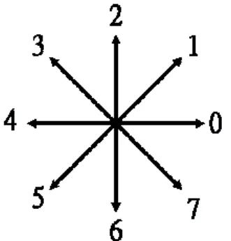
(2) point independently.. the. curvature. κ=dθ/ds.. However,. the. above. Ray and Ray [8] indicated that an asymmetric. definition does not hold for a digital curve, due to. region of support is more reasonable and more. that there exist no mathematical definition for the. natural than a symmetric region of support. That is,. digital curve. Therefore, most of the existing. the left support and the right support for the point of. algorithms focus on curvature estimation by use of. the interest are not the same. Once the left support. the information of the neighbors. The presented. and the right support have been determined, the. method intends to determine the region of support for. k-l-cosine value is computed as the estimated. each point quickly.. curvature.. A digital closed curve C can be defined as the set. Cornic [3] addressed that, as for the Teh and Chin algorithm, the Ray and Ray algorithm is not robust in presence of noise. Evaluating the significant of point. consisting of n consecutive points. C = {Pi (xi ,yi )|i = 1,2 ,...,n},. (1). by the other points of the curve is proposed. He used. where n is the number of points, Pi is the i th point. the chain code properties of digital straight line to. with coordinate (xi, yi), and points Pi-1 and Pi+1 are. compute two vectors of significance. The dominant. neighbors of point Pi (modulo n).. points are then detected by a logical unction.. The Freeman’s chain code [5] of C consists of the. However, the computation is complex in determining. n chain codes and is denoted as c1c2…cn, where. left support and right support. In addition, it is. ci=ci±n and all indices are modulo n. All integers are. difficult to select a best logical function (strategy) on. modulo n. That is, each of the vectors is assigned to. the dominant point identification step. In this paper, we focus on developing a simple. an integer ci varying from 0 to 7, where. 1 4. π ci is the. method to determine an asymmetric region of. angle between the x-axis and the vector, for i=1,. support. The break point detection procedure is. 2, …, n (see Fig. 1).. applied to find the candidates of dominant points on the curve. The left and right regions of support are then determined in the same time. The experimental results show that the method is efficient and effective in detecting dominant points. In section 2, we will illustrate the dominant point detection methods as well as the proposed algorithm. Section 3 will present the experimental results of the new strategy. Some concluding remarks are then given in section 4.. Fig. 1. Freeman’s chain codes.. 2. Dominant Point Detection. It is reasonable to exclude those linear points,. The points with local maximum curvature are. since the points on straight line cannot be considered. considered as the dominant points. For a continuous. as the dominant points [16]. The survived points are. curve, curvature of a point is defined as the rate of. candidates of dominant points and denoted as the. change of slope as a function of arc length. That is,. break points. The linear points can be removed by.

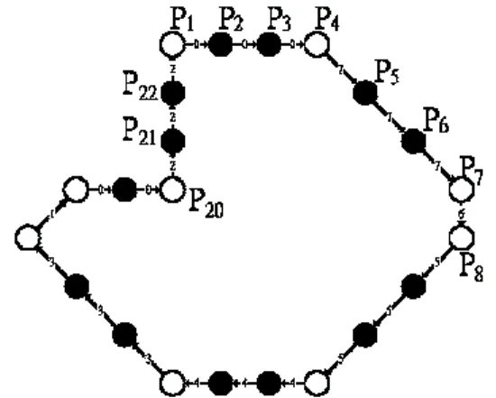
(3) tracking the chain codes. The following rule is. information of break points while determining the. applied to identify those linear points.. region of support. The determination of support can be done by use of its previous and next break points. Rule 1. If ci-1=ci, then the point Pi is a linear point.. as the left and right supports, respectively. The points. Otherwise, it is a break point.. between previous break point and the next break point consist the region of support for the point of. An example of chain-coded curve is shown in Fig.. interest. For example, the points P4 and P8 are the left. 2. The points P2 and P3 are linear points. and right supporting points of the point P7,. (c1=c2=c3=0), and the points P1 and P4 are break. respectively (see Fig. 2). The region of support for. points (c22=2≠0=c1 and c3=0≠7=c4). By tracking the. the point P7 is defined as the set of points P4 to P8.. chain codes of the curve, the break points can be located. They are marked as “○” in Fig. 2.. Suppose that there are m break points on the curve and the i th break point Bi is the bi th point on the curve. The lengths of left and right regions of support for Bi are denoted as li and ki, respectively. The region of support of each break point can be determined by the following rules. Rule 2. For the break point Bi, the left arm. terminated at Bi-1 and the right arm terminated at Bi+1. The length of left region of support li=bi-bi-1, while the length of right region of support ki=bi+1-bi. The length of region of support ri=bi+1-bi-1+1. The region Fig. 2. Break point detection by the relationship between points Pi and the chain codes ci on the curve. Chain codes: 0007776555444333100222. (○) break. of support for the break point Bi consists of the set. {Pb ,...,Pb ,..., Pb } . i i −1 i +1. point; (●) linear point.. The k-l-cosine value is used to estimate curvature of It will reduce the computation time both in determination of support region and curvature. each break point. For the break point Bi, it is defined as. estimation, if only the set of break points are considered as the possible dominant points. In fact, once the break points have been identified, the left support as well as the right support for each point can be determined quickly. The considering region of support is asymmetric as in Ray and Ray [8]. That is, the length of the right region of support and that of the left region of support should be determined independently. An intuitive approach is to use the. v v aik • bik cosikl = v v , aik bik v where a = (xb − xb ,yb − y b ) and ik i i +1 i i +1 v bik = (xb − xb ,yb − yb ) . i i −1 i i −1. (2).

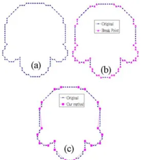
(4) Once the k-l-cosine values have been determined,. Step 4. Identify the dominant points by Rule 3.. the next step is to identify the dominant points. Five conditions of suppressing the break point Bi from the set of candidates of dominant points are given as follows.. 3. Experimental Results. The proposed method has been applied to four commonly used curves in many studies [8]. They are. Condition A. cosikl < ε. (3). the chromosome curve (Fig. 3(a)), infinity curve (Fig.. Condition B. cosikl < cosjkl, for j=i-1 or i+1. (4). 4(a)), leaf curve (Fig. 5(a)), and semicircle curve (Fig. Condition C. cosikl = cosi-1,kl and ri < ri-1. (5). 6(a)). In the experiment, the curvature threshold ε is. Condition D. cosikl = cosi+1,kl and ri < ri+1. (6). set to –0.5. By tracking the chain codes, the break. Condition E. cosikl = cosi+1,kl and ri = ri+1. (7). points can be determined, and they are shown in Figs. 3(b), 4(b), 5(b), and 6(b), for the four types of curves,. It is necessary to suppress those break points. respectively.. whose curvature less than a preset threshold ε (Condition A). Condition B indicates that a dominant point should have local maximum curvature. For two neighboring break points, the point with smaller length region of support is removed (Conditions C and D). Further, if two consecutive points has the same curvature and the same length region of support, discard the later one (Condition E). The survived break points with local maximum over its region of support are denoted as the dominant points. Therefore, we can locate of dominant points by the following rule.. Fig. 3. The chromosome curve: (a) original, (b) break points, and (c) dominant points.. Rule 3. If one of the Conditions A to E is satisfied,. then the break point Bi is removed from the set of candidates of dominant points. Overall, the proposed method is summarized as follows: Step 1. Extract break points from Freeman’s chain codes by Rule 1. Step 2. Determine region of support for each break point (ki and li, i=1, 2, ..., m) by Rule 2. Step 3. Compute the estimated curvatures for all of the break points (cosikl, i=1, 2, ..., m) by Eq.. Fig. 4. The infinity curve: (a) original, (b) break. (2).. points, and (c) dominant points..

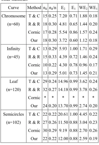
(5) In order to assess the performance of the proposed method, six performance evaluation criteria. desirable to have the number of dominant points as small as possible.. were used in the experiment. Most of them were used. (2) Inverse of compression ratio (nd/n): One of the. by Conic [3]. They are the number of the dominant. objectives for dominant point detection is to. points, inverse of compression ratio, sum of square. reduce the amount of data. The smaller the. error, maximum error, weighted sum of square error,. inverse of compression ratio is, the more. and weighted maximum error.. effective in data reduction the method is. (3) Sum of square error (E2): This criterion assesses the distortions caused by the approximated curve. The smaller the sum of square error is, the better descriptive ability the method is. It is defined as n 2 E = å e , 2 i =1 i. (8). where ei is the distance from Pi to the approximated segment. (4) Maximum error (E1): This criterion assesses the approximated errors. The smaller the maximum error is, the better fitness the method is. It is defined as. Fig. 5. The leaf curve: (a) original, (b) break points, and (c) dominant points.. n E = max {e }. 1 i i =1. (9). (5) Weighted sum of square error (WE2): The weighted sum of square error is to compromise the compression ratio and the sum of square error. It is defined as n WE 2 = d × E 2 n. (10). (6) Weighted maximum error (WE1): The weighted maximum. error. is. to. compromise. the. compression ratio and the maximum error. It is defined as n WE1 = d × E1 n. (11). Fig. 6. The semicircle curve: (a) original, (b) break points, and (c) dominant points.. The objective for detecting dominant points is to minimize all of the six criteria, whereas it seems to. (1) Number of the dominant points (nd): It is. be impossible to obtain an optimal solution. The.

(6) objective of this paper is not to propose an optimal. smaller sum of square error than that of Cornic’s. solution to dominant point detection. Alternatively, it. method. In addition, our method detect the same. attends to show that the new method is very simple. number of dominant points to that of Teh & Chin’s. and it can improve the performance of the family of. method, whereas it is superior to Teh & Chin’s. region of support determining algorithms. The. method since all of the other criteria of our method. experimental results of our method and of the other. are smaller than that of Teh & Chin’s method. The. methods are listed in Table 1. The presented result of. new method has higher compression ratio than that of. the Conic’s method is that of the best performance. Ray & Ray’s method, and it has the smaller values of. indicated in his paper.. WE1 and WE2. The proposed method has the smallest nd for the leaf curve (Cornic’s method doest not. Table 1. Results of the proposed method and of the. provide the result in his paper). Further, it has the. other methods.. best performance on all of the other criteria while E1 WE2 WE1. comparing to the other methods. That is, the new. Chromosome T & C 15 0.25 7.20 0.71 1.88 0.18. method can detect a set of the most significant points. Curve. Method nd nd/n. (n=60). E2. R & R 18 0.30 4.81 0.65 1.44 0.20. that has the minimum number of points and it can. Cornic 17 0.28 5.54 0.86 1.57 0.24. approximate the original curve very well. Again, the. 18 0.30 3.72 0.60 1.12 0.18. same finding can be seen for the semicircle curve.. Infinity. T & C 13 0.29 5.93 1.00 1.71 0.29. Especially, it detects a set of symmetric dominant. (n=45). R & R 15 0.33 4.39 0.72 1.46 0.24. points for the semicircle curve.. Our. Cornic 10 0.22 4.30 0.78 0.96 0.17. The detected dominant points superimposed to the. 13 0.29 5.01 0.73 1.45 0.21. respective original curves are shown in Figs. 3(c),. Leaf. T & C 29 0.24 14.96 0.99 3.62 0.24. 4(c), 5(c), and 6(c), respectively. Overall, the new. (n=120). R & R 32 0.27 14.18 0.99 3.78 0.26. method proposes a simple method to determine. Our. Cornic * Our. *. *. *. *. *. 24 0.20 13.70 0.99 2.74 0.20. Semicircles. T & C 22 0.22 20.61 1.00 4.45 0.22. (n=102). R & R 27 0.26 11.50 0.88 3.04 0.23. region of support for each point, and it perform very well while comparing to the other methods.. 4. Conclusions. Cornic 30 0.29 9.19 0.88 2.70 0.26. Dominant points are those points that have. 22 0.22 12.00 0.88 2.59 0.19. curvature extreme on the curve and they can suitably. Our * not provided. describe the curve for both visual perception and recognition. Teh-Chin [13] proposed an adaptive. For the chromosome curve, Teh & Chin’s method. method to determine region of support for each point.. detects the minimum number of dominant points, but. Ray and Ray [8] further suggested that an. it has the largest E2. It is seen that our method has the. asymmetric region of support is more reasonable and. smallest E2, E1, WE2, and WE1. That is, our method. more natural than a symmetric region. Cornic [3]. has the better performance than the other methods.. used the information of the other points to determine. For infinity curve, Cornic’s method seems to have. the support region.. the best performance. However, our method has. In this paper, the concept of linearity is used to.

(7) find a set of break points. The asymmetric region of. detection of dominant points and polygonal. support for each break point is then determined in the. approximation of digitized curves”, Pattern. same time. The proposed method is fast and it needs. Recognition Letters, 13, 1992, pp. 849-856.. no input parameters. From the experimental results, it. 9.. Ray, B. K. and Ray,. K. S., “A new. is show that the proposed method is efficient and. split-and-merge. technique. for. polygonal. effective in detecting dominant points.. approximation of chain coded curves”, Pattern Recognition Letters, 16, 1995, pp. 161-169. 10. Rosenfeld, A. and Johnston, E., “Angle detection. Acknowledgements. This paper is partially supported by National Science. on digital curves”, IEEE Trans. Computers, 22,. Council, ROC under grant no. NSC 88-2213-E-214-. 1973, pp. 875-878. 11. Rosenfeld, A. and Weszka, J. S., “An improved. 016.. method of angle detection on digital curves”, IEEE Trans. Computer, 24, 1975, pp. 940-941.. References. 1.. 2.. 3.. Ansari, N. and Delp, E. J., “On detection. 12. Sklansky, J. and Gonzalez, V., “Fast polygonal. dominant points”, Pattern Recognition, 24, 1991,. approximation of digitized curves”, Pattern. pp. 441-450.. Recognition, 12, 1980, pp. 327-331.. Attneave, F. “Some information aspects of visual. 13. Teh, C. H. and Chin, R. T., “On the detection of. perception”, Psychological Review, 61, 1954, pp.. dominant points on digital curves”, IEEE Trans.. 183-193.. Pattern Analysis and Machine Intelligence, 11,. Cornic, P., “Another look at the dominant point. 1989, pp. 859-872.. detection of digital curves”, Pattern Recognition 4.. Letters, 18, 1997, pp.13-25.. method for polygonal approximation of digitized. Dunham, J. G., “Optimum uniform piecewise. curves”, Computer Vision, Graphics, and Image. linear approximation of planar curves”, IEEE. Processing, 28, 1984, pp. 220-227.. Trans. 5.. Pattern. Analysis. and. Machine. 7.. 8.. 15. Wang, M. J., Wu, W. Y., Huang, L. K., and Wang,. Intelligence. 8, 1986, pp. 67-75.. D. M., “Corner detection using bending value”,. Freeman, H., “On the encoding of arbitrary. Pattern Recognition Letters, 16, 1995, pp.. geometric. 575-583.. configurations”,. IRE. Trans.. Electronics Computing, 10, 1961, pp. 260-268. 6.. 14. Wall, K. and Danielsson, P. E., “A fast sequential. 16. Wu, W. Y. and Wang, M. J., “Detecting the. Kankanhalli, M. S., “An adaptive dominant. dominant. points. by. the. curvature-based. point detection algorithm for digital curves”,. polygonal approximation”, CVGIP: Graphical. Pattern Recognition Letters, 14, 1993, pp.. Models and Image Processing, 55, 1993, pp.. 385-390.. 79-88.. Ramer, U., “An iterative procedure for the. 17. Yin, P. Y., “Genetic algorithms for polygonal. polygonal approximation of plane curves”,. approximation of digital curves”, International. Computer Graphics and Image Processing, 1,. Journal of Pattern Recognition and Artificial. 1972, pp. 244-256.. Intelligence, 13, 1999, pp. 1061-1082.. Ray, B. K. and Ray, K. S., “An algorithm for.

(8)