The Influence of Artificial Cut-off on a Monitoring System and the Water Quality of the Keelung River

The influence of artificial cutoff on a monitoring system

and the water quality of the Keelung River

S.L. Lo, J.T. Kuo and S.M. Wang

Graduate Institute of Environmental Engineering, National Taiwan University, 71 Chou-Shan Rd., Taipei, Chinese Taiwan

Abstract The purpose of this study was to design a water quality monitoring network for the Keelung River in order to evaluate the effects of artificial cutoff across two bend channels. A steady-state water quality model was used to simulate the BOD and DO curves. The Kriging theory was applied to select the optimal locations for a water quality monitoring network. The sampling frequency was determined by the coefficients of variation of water quality and by considering the significance level and confidence interval. After calibration and verification of the water quality model, the model was applied and the simulation results indicated that the values of DO in the new channel would be higher than those of the old channel reaches. The critical point of the oxygen sag curve would shift to the mouth of river under Q₇₅low-flow conditions, and the BOD values in the new channel would also slightly increase. The results further indicated that more monitoring stations would be needed in the downstream reaches.

Keywords Artificial cutoff; Kriging theory; monitoring system; water quality modeling

Introduction

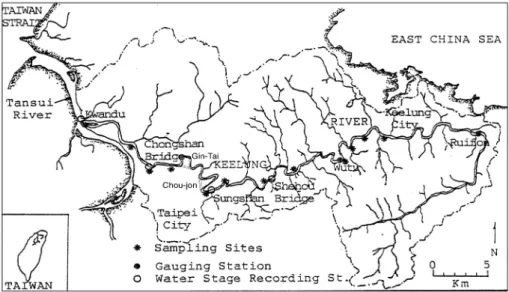
The Keelung River has the longest tidal excursion and worst pollution problems of the three tributaries of the Tansui River. Artificial cutoff of the Keelung River (Figure 1, Gin-Tai reach and Chou-jon reach) will change the hydrologic, hydraulic and water quality characteristics of the river. The Tansui River clean-up project will increase the number of households connected to sewers of the separate system, which, combined with both an interception system and sewage treatment plant, will reduce pollution to the river. Although the project will reduce the pollutant loading, it will intercept the natural base flow and, hence, affect the improvement of water quality.

A well planned monitoring system can effect proper, timely measures and resolutions on water quality monitoring as well as pollution control. In the past, the design of monitoring stations was generally based on personal experience. Lo et al. (1996) analyzed the spatial variation from the simulation results of river water quality models of the Keelung River and used Kriging theory to select the optimal locations of a water quality monitoring network. The sampling frequency was determined by the proportional sampling method with respect to variances of water quality, significance level and confidence interval. This study investi-gates the effects of artificial cutoff of the Keelung River on a monitoring system and on the river water quality. The results provide decision-makers with several options for selecting optimal conditions applicable to the actual environment.

River water quality model

Under steady-state conditions, one-dimensional equations for Biochemical Oxygen Demand (BOD) and Dissolved Oxygen (DO) of a river can be expressed as

(1)

Water Science and Technology

Vol 46 No 11–12 pp 231–236 © IWA Publishing 2002 231 − ∂

( )

∑

A is the cross-sectional area of flow (m2), x is the flow distance (m), Q is the flow rate (CMD), L is the ultimate carbonaceous BOD (CBOD, mg/L), D is the oxygen deficit

(mg/L), K_ris the BOD removal rate (1/day), K_dis the deoxygenation coefficient of BOD

(1/day), K_ais the reaeration coefficient (1/day), E is the longitudinal dispersion coefficient (m2/day), and S₁is the BOD loading (kg/m3/day) and S₂represents all other sources and sinks of DO (kg/m3_{/day). To solve these two equations, the river reach is initially divided} into separate segments. Each segment is then treated as a completely mixing zone. The finite difference method can be applied to the numerical analysis to obtain the BOD and oxygen deficit in each river segment (Robert and Mueller, 1987).

The total length of the Keelung River was 81 km and was reduced to 76.1 km after artifi-cial cutoff. The new length was segmented into 31 reaches as before (Lo et al., 1996). The locations of reach numbers 25–31 remained the same, but the locations of reach numbers 20–24 shifted from 19.6, 18.5, 17.5, 14.7 and 11.9 km to 16.1, 15.0, 13.9, 12.5 and 11.5 km, respectively. The locations of numbers 1–19 all shifted downward by 4.9 km. Before artificial cutoff, stream velocity and the depth of each reach were computed from stream flow by the method of “discharge coefficients” (Lo et al., 1996). After artificial cutoff, stream velocity and the depth of the new channel reaches were computed from the Manning formula. The slope of artificial channel became 1.5/10,000, and the side slope of the trape-zoidal cross section became 1:4. The roughness coefficient of the Manning formula was chosen to be 0.015.

The values of the model parameters were determined by laboratory or in situ

experi-ments and further adjusted during model calibration. The value of K_awas calculated from

the O’Connor and Dobbins equation. Because new channel reaches have much higher

velocity and shallow depth, the K_avalues of these reaches are much higher than those of

other reaches. The rates of benthic oxygen demand S_dwere determined by an in situ benthic

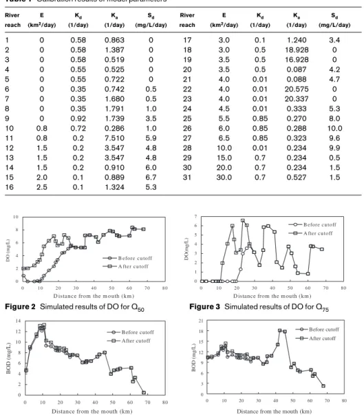
respirometer. The results showed no significant S_dfor the non-tidal and new channel reach-es of the Keelung River, but, for the tidal reachreach-es, the valureach-es of S_dranged from 1.0 to 10.0 mg/L/day. All calibration results of the model parameters are shown in Table 1.

The simulated DO values before and after artificial cutoff under Q₅₀and Q₇₅are shown

S.L. Lo

et al.

232

Figure 1 Map of the Keelung River in Northern Taiwan

− ∂

( )

∑

in Figure 2 and Figure 3, respectively. In Figure 2, the DO values of downstream reaches after artificial cutoff increase by approximately 2 mg/L. In Figure 3, the point of minimum DO of the oxygen sag curve shifts downstream by about 9–10 km. The improvement in the

DO values of downstream reaches results from much higher reaeration coefficients (K_a).

The simulated BOD values increased slightly for downstream reaches after artificial

cutoff (Figures 4 and 5). Under Q₇₅flowrate, BOD values increased by about 0.3–0.8 mg/L.

Because the channel length is reduced and because the velocity increases after artificial cut-off, the biological decomposition time is shortened, causing the BOD values of down-stream reaches to increase slightly.

Optimization of the monitoring network

The Kriging method provides relatively robust estimates of random functions and their variances. Matheron (1963) pointed out that the variance of estimation can be computed before the actual measurements are available and suggested that Kriging can be applied to locate measurement points in such a way that the estimation variance is minimized. The

S.L. Lo et al. 233 0 2 4 6 8 1 0 0 1 0 2 0 3 0 4 0 5 0 6 0 7 0 8 0 D istance from the m outh (km )

DO (mg/L) B e fo re cu to ff A fte r c u to ff 0 1 2 3 4 5 6 7 0 10 20 30 40 50 60 70 80

D istance from the m outh (km )

DO(mg/L)

B efore cu toff A fter cu toff

Figure 2 Simulated results of DO for Q₅₀ Figure 3 Simulated results of DO for Q₇₅

0 2 4 6 8 10 12 14 0 10 20 30 40 50 60 70 80

Distance from the mouth (km)

BOD (mg/L) Before cutoff After cutoff 0 3 6 9 12 15 18 21 0 10 20 30 40 50 60 70 80

Distance from the mouth (km)

BOD (mg/L)

Before cutoff After cutoff

Figure 4 Simulated results of BOD for Q₅₀ Figure 5 Simulated results of BOD for Q₇₅ Table 1 Calibration results of model parameters

River E Kd Ka Sd River E Kd Ka Sd

reach (km2_{/day) (1/day) (1/day) (mg/L/day) reach (km}2_{/day) (1/day) (1/day) (mg/L/day)}

1 0 0.58 0.863 0 17 3.0 0.1 1.240 3.4 2 0 0.58 1.387 0 18 3.0 0.5 18.928 0 3 0 0.58 0.519 0 19 3.5 0.5 16.928 0 4 0 0.55 0.525 0 20 3.5 0.5 0.087 4.2 5 0 0.55 0.722 0 21 4.0 0.01 0.088 4.7 6 0 0.35 0.742 0.5 22 4.0 0.01 20.575 0 7 0 0.35 1.680 0.5 23 4.0 0.01 20.337 0 8 0 0.35 1.791 1.0 24 4.5 0.01 0.333 5.3 9 0 0.92 1.739 3.5 25 5.5 0.85 0.270 8.0 10 0.8 0.72 0.286 1.0 26 6.0 0.85 0.288 10.0 11 0.8 0.2 7.510 5.9 27 6.5 0.85 0.323 9.6 12 1.5 0.2 3.547 4.8 28 10.0 0.01 0.234 9.9 13 1.5 0.2 3.547 4.8 29 15.0 0.7 0.234 0.5 14 1.5 0.2 0.910 6.0 30 20.0 0.7 0.234 1.5 15 2.0 0.1 0.889 6.7 31 30.0 0.7 0.527 1.5 16 2.5 0.1 1.324 5.3

Kriging method has been applied to the optimal monitoring network design for groundwa-ter management (Hughes and Lettenmaier, 1981; Carrera et al., 1984; Loaiciga, 1989). Assuming there are n measuring points, x₁, x₂..., x_n, the corresponding measured data are

Z(x₁), Z(x₂),..., Z(x_n), respectively. If x₁, x₂..., x_nare located in the same region or subdo-main, then average water quality in region V in the Kriging estimation can be written as

where V denotes the length, area or volume of the region V in one-, two-, or three-dimen-sional space, respectively. The estimate Z* of the average value Z_aveis considered to be a weighted average of the n available data:

where λ_iare weighting factors or Kriging coefficients. The Kriging method is purposed on

an accurate estimation of Z_aveby Z*. Thus, the Kriging linear estimate should satisfy two

main conditions: (i) it should be unbiased, which means the expectation value of estimated

Z* is equal to the expectation value of average measured Z_ave, E[Z*] = E[Z_ave], with Journel and Huijbregts (1978) proving that the unbiased condition is satisfied if

and (ii) it should have minimum variance, meaning Min E[(Z* – Z_ave)2_{]. Therefore, in order} to comply with these two conditions of Kriging theory, the minimum E[(Z* – Z_ave)2_{] is used} as the objective function, and Eq. (5) is the constrained equation. This nonlinear program-ming can be performed using Lagrange multipliers and leads to the solution of the Kriging equations (Carrera et al., 1984). The “branch and bound” algorithms can be used for select-ing optimal locations from a discrete set of possible measurement stations (Nakamura and Riley, 1981; Carrera et al., 1984).

If monitoring stations are designed to detect worsening water quality conditions, river water quality can be better managed and controlled. From the flow-duration curve recorded at Wutu station in consideration of medium/low flow such as Q₅₀, Q₆₀, Q₇₀, Q₇₅, Q₈₀, Q₉₀, etc., it was found that the corresponding flowrates were 9.10, 6.10, 4.30, 3.41, 2.80 and

1.33 m3_{/sec. Using four different water temperatures (30°C, 28°C, 25°C and 20°C), 24}

dif-ferent combinations of distinct conditions were simulated. The results of the BOD and DO distributions in each river reach are shown in Figure 6 and Figure 7, respectively. Compared with the distributions before artificial cutoff, the BOD results showed similar distributions, but the DO distributions were quite different. Because the DO model already includes BOD results, and because there is a great BOD fluctuation at the 9th and 10th reaches as a result of wastewater from the Liutu industrial zone and sewage from northern Wutu, the optimal monitoring locations are determined by the DO simulation results.

S.L. Lo et al. 234 Z V Z x dx ave v = 1

_∫

∑

∑

Distance from the mouth (km)

BOD (mg/L) 0 2 4 6 8 1 0 0 1 0 2 0 3 0 4 0 5 0 6 0 7 0 D i s t a n c e f r o m t h e m o u t h ( k m ) DO (mg/L)

Figure 6 Simulated results of BOD for medium/low

Figure 7 Simulated results of DO for medium/low

(3)

(4)

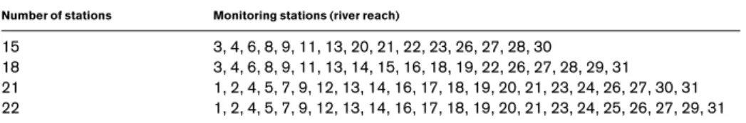
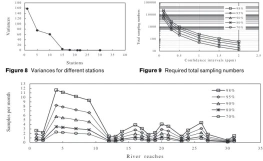
Proceeding with the selection of monitoring stations, the simulated DO data of each river reach were input into an optimization model. Figure 8 shows the calculated variances for different numbers of monitoring stations. The fewer the stations, the larger the variance, and vice versa. The optimization results for 15, 18, 21 and 22 monitoring stations are shown in Table 2. As shown by the decreasing trend of variances, 21 monitoring stations are needed and more monitoring stations should be set up downstream.

Sampling frequency

After the optimal locations of the monitoring stations are chosen by Kriging theory, the sampling frequency should be determined. Provided that the water quality of each monitor-ing station is normally distributed,

Z = (x – µ) / σ (6)

where Z is the standardized random variable, x is a random variable, µ is the mean value and σ is the standard deviation. Assuming that there is a normal distribution with a significance level of α% and the radius of confidence interval is R, then

R = S_xZ_{α /2}/ √N (7)

where S_xis the standard deviation of samples, N is the number of samples and Z_α/2is the dis-tribution coefficient of the normal disdis-tribution. Proportional sampling means that the num-ber of samples needed in each station is distributed in proportion to the variance of sample data in each station (Ward et al., 1979). From this, the greater the variance, the greater the sampling frequency, and vice versa:

where T is the total number of samples in all stations and N_iis number of samples in the ith station. Substituting Eq. (8) into Eq. (7) results in the following equation:

From Eq. (9) the total sampling number T can be determined after significance level and confidence interval have been chosen and water quality variance of each station been calcu-lated. Furthermore, the sampling frequency in each station can be obtained from Eq. (8).

In this study, confidence limits of 98%, 95%, 90%, 80% and 70%, with confidence inter-vals of 0.1, 0.3, 0.5, 1, 1.5 and 2 ppm, respectively, were chosen. The required sampling num-ber increases when the confidence limit is increased and the confidence interval is decreased. Figure 9 shows the required total sampling numbers for 21 stations with respect to different confidence limits and intervals. When the confidence interval is decreased to 0.3 or even 0.1 ppm, a much higher sampling frequency is required. However, when the confidence interval is increased to 1.5 or 2.0 ppm, the sampling frequency becomes too low. Sampling frequen-cies of high and low extremes are not cost-effective. As a result, this study chose a confidence interval of 0.5 ppm for discussion. The results at different confidence limits are given in

S.L. Lo

et al.

235

Table 2 Optimal monitoring stations

Number of stations Monitoring stations (river reach)

15 3, 4, 6, 8, 9, 11, 13, 20, 21, 22, 23, 26, 27, 28, 30 18 3, 4, 6, 8, 9, 11, 13, 14, 15, 16, 18, 19, 22, 26, 27, 28, 29, 31 21 1, 2, 4, 5, 7, 9, 12, 13, 14, 16, 17, 18, 19, 20, 21, 23, 24, 26, 27, 30, 31 22 1, 2, 4, 5, 7, 9, 12, 13, 14, 16, 17, 18, 19, 20, 21, 23, 24, 25, 26, 27, 29, 31 N S S T i xi xi =

∑

∑

Figure 10, which shows that if the confidence interval is 0.5 ppm, the sampling must be per-formed 1–4 times (2 or 3 times is the best) per month to arrive at the objective.

Conclusions

The simulation results indicate that the DO values of downstream reaches after artificial cut-off increased by approximately 2 mg/L. The critical point of the oxygen sag curve shifts to

the mouth of river by about 9–10 km under Q₇₅low flow conditions. Using Kriging theory in

the selection of monitoring stations shows that the required number of stations is 21 and that more monitoring stations should be set up downstream. The optimal sampling frequency is 2–3 times per month at 0.5 ppm DO confidence interval and 90% confidence limit.

Acknowledgement

This study was supported by the National Science Council, Chinese Taiwan, under contract NSC 80-0421-E002-10Z.

References

Carrera, J., Usonoff, E. and Szidarovszky, F. (1984). A method for optimal observation network design for groundwater management. J. Hydrol., 73, 147–163.

Hughes, J.P. and Lettenmaier, D.P. (1981). Data requirements for Kriging: Estimation and network design. Water Resour. Res., 17, 1641–1650.

Journel, A.G. and Huijbregts, Ch. J. (1978). Mining Geostatistics. Academic Press, New York, N. Y. Lo, S.L., Kuo, J.T. and Wang, S.M. (1996). Water quality monitoring network design of Keelung river,

northern Taiwan. Wat. Sci. Tech., 34(12), 49–57.

Loaiciga, H.A. (1989). An optimization for groundwater quality monitoring network design. Wat. Resour. Res., 25, 1771–1782.

Matheron, G. (1963). Traite de Geostatistique Appliquee, vols. 1 and 2, Editions Technip, Paris. Nakamura, M. and Riley, J.M. (1981). A multiobjective branch and bound method for network-structured

water resources planning problems. Wat. Resour. Res., 17, 1349–1359.

Robert, V.T. and Mueller, J.A. (1987). Principle of Surface Water Quality Modeling and Control. Harper and Row Publishers, New York, N. Y.

Ward, R.C., Loftis, J.C., Nielsen, K.S. and Anderson, R.D. (1979). Statistical evaluation of sampling frequencies in monitoring networks. J. Wat. Pollut. Control Fed., 51, 2292–2300.

S.L. Lo et al. 236 0 2 0 4 0 6 0 8 0 1 0 0 1 2 0 1 4 0 1 6 0 1 8 0 0 5 1 0 1 5 2 0 2 5 3 0 3 5 4 0 S ta tions Variances 1 0 1 0 0 1 0 0 0 1 0 0 0 0 1 0 0 0 0 0 0 0 .5 1 1 .5 2 2 .5 C o n fi d e n c e i n t e r v a l s ( p p m )

Total sampling numbers

9 8 % 9 5 % 9 0 % 8 0 % 7 0 %

Figure 8 Variances for different stations Figure 9 Required total sampling numbers

0 1 2 3 4 5 6 7 8 9 1 0 1 1 1 2 1 3 0 5 1 0 1 5 2 0 2 5 3 0 3 5 R iv e r r e a c h e s

Samples per month

9 8 % 9 5 % 9 0 % 8 0 % 7 0 %