國 立 交 通 大 學
電信工程研究所
博 士 論 文
使用超穎材質以降低特定吸收比及交互
方向內隱式時域有限差分法之穩定度改善
SAR Reduction with Metamaterials and
Stability Improvement of ADI-FDTD
研 究 生:黃 竣 南
指導教授:鍾世忠
使用超穎材質以降低特定吸收比及交互
方向內隱式時域有限差分法之穩定度改善
SAR Reduction with Metamaterials and
Stability Improvement of ADI-FDTD
研究生: 黃竣南 Student: Jiunn-Nan Hwang
指導教授:鍾世忠 博士 Advisor: Dr. Shyh-Jong Chung
國立交通大學
電信工程研究所
博士論文
A Dissertation
Submitted to Department of Communication Engineering
College of Electrical and Computer Engineering
National Chiao Tung University
in Partial Fulfillment of the Requirements
for the Degree of Doctor of Philosophy
in
Communication Engineering
Hsinchu, Taiwan
摘要
目前行動通訊裝置使用人數日與俱增,而人們也開始關心手機電磁輻射對人體 的影響。其中,藉由特定吸收效率可以瞭解人頭電磁能量吸收的多寡。目前,時 域有限差分法已應用於人頭特定吸收效率的計算。最近,超穎材質由於具有特殊 物理特性而引起研究人員對其興趣。超穎材質為人造材質,由於其介電係數與導 磁係數為負值,因此超穎材質電磁傳輸特性不同於一般材質。 在本研究中,我們將使用超穎材質以減低人頭與天線間交互電磁現象。首先, 我們利用時域有限差分法結合 Drude 模型來模擬超穎材質。在模擬中,超穎材質 置於天線與人頭間。從模擬結果可知,藉由擺放超穎材質可以有效減低人頭的特 定吸收效率。我們也探討擺放超穎材質對於天線影響。藉由適當擺放超穎材質, 超穎材質對於天線輻射能量和天線場型影響不大。而我們進一步探討擺放位置, 尺寸大小,超穎材質介質係數對於減低特定吸收效率的影響。超穎材質可以藉由 設計分離式環形共振器來實現。在本研究中,我們設計分離式環形共振器,使其 工作頻率為 900 MHz 和 1800 MHz。設計流程也將詳細描述。我們將設計的分離 式環形共振器置於天線與介質體中間,從結果可以發現介質體的特定吸收效率將 會減低。此研究可以提供減低特定吸收效率的方法。 在研究中,我們也發展無條件穩定 ADI-FDTD 模擬方法。我們發現,當使用吸 收邊界於 ADI-FDTD 時,可能會造成演算法不穩定問題。首先,我們探討 Mur 吸 收邊界於 ADI-FDTD 的數值穩定分析。在此演算法中,電磁波傳播方向將會影響 該演算法穩定度。從模擬結果可知,該演算法只有在波行進方向為 0 度,45 度, 90 度時會穩定。我們也推導出該演算法數值色散關係式。發現此演算法數值不 穩定是無法改善。接著,我們探討應用分離場完美匹配層於 ADI-FDTD 的穩定度 分析。穩定度理論分析可以藉由推導穩定矩陣實現。我們發現應用分離場完美匹 配層於 ADI-FDTD 會造成數值不穩定結果。完美匹配層中電導會影響該演算法穩 定度。因此,我們提出改良完美匹配層電導,以改善該演算法穩定度。最後藉由 數值模擬可以驗證分離場完美匹配層和 Mur 吸收邊界於 ADI-FDTD 的數值不穩定 效應。CN-FDTD 為另一種無條件穩定演算法。ADI-FDTD 與 CN-FDTD 差別只是二階 近似項。在本研究中,我們將分析分離場完美匹配層,非分離場完美匹配層,複 數頻率轉換完美匹配層對於 ADI-FDTD 與 CN-FDTD 的影響。我們發現 ADI-FDTD 不穩定是二階近似項所造成。藉由此研究可以提供未來發展應用於 ADI-FDTD 簡 潔穩定的完美匹配層。由於在 ADI-FDTD 中,其時間步階不受穩定法則限制,故 該演算法非常適合模擬超大型積體電路。藉由改良完美匹配層,我們發現所提出 的演算法可以有效率以及準確模擬超大型積體電路時域與頻域電磁特性。 在多天線系統中,增加天線隔絕度為重要參數。在本研究中,藉由在兩天線間 增加一耦合元件,可以有效增加隔絕度。此耦合元件優點為不增加額外天線面 積。在研究中,耦合元件尺寸對於天線隔絕度效率與共振頻率也將做進一步探討,經由天線量測結果,所提出的耦合元件可以增加天線 15dB 的隔絕度,增加 耦合元件對於天線場型亦只有減少 1dB 增益以內的影響
Abstract
The use of the mobile devices has been growing rapidly in the global communities. The influence of electromagnetic (EM) waves from cellular phones on the human head has been widely discussed recently. The specific absorbing rate (SAR) is a defined parameter for evaluating power deposition in human tissue. The finite-difference time-domain (FDTD) is widely used to study the peak SAR in the human head. Recently, metamaterials have inspired great interests in their unique physical properties and novel application. Metamaterials denote artificially constructed materials having electromagnetic properties not general found in nature. Two important parameters, electric permittivity and magnetic permeability determine the response of the materials to the electromagnetic propagation.
In this work, we use the metamaterials to reduce the EM interaction between the antenna and human head. Preliminary simulation of metamaterials is performed by FDTD method with lossy Drude model. The metamaterials are placed between the antenna and human head. From the simulation result, it is found that the peak SAR in the human head can be reduced with the placement of metamaterials. We also study the antenna performance with metamaterials. The antenna radiated power and antenna pattern can be less affected with placement of metamaterials properly. The effects of placement position of metamaterials, metamaterials size, and the medium parameters of metamaterials on the SAR reduction effectiveness are investigated. The metamaterials can be constructed from split ring resonators (SRRs). In this work, we also design the SRRs operated at 900 MHz and 1800 MHz. The design procedure of the SRRs is described. The designed SRRs are placed between the antenna and a dielectric cube. It is found that the peak SAR in the dielectric cube is reduced significantly. This study can provide useful methodology for SAR reduction.
In this work, we develop the alternating direction implicit (ADI) finite-difference time-domain (FDTD) method. However, when employing the absorbing boundary conditions (ABCs) for ADI-FDTD method, this scheme can lead to instability. First, the stability analysis of the Mur’s ABC for ADI-FDTD method is also studied. The effect of the wave propagation direction on the stability of this scheme is investigated. It is found that this scheme can be stable only when the incident wave directions are 0 degree, 45 degree, and 90 degree. We also derive the dispersion relation of this scheme. The instability of this scheme can not be avoided. Then, the stability analysis of split-field perfectly matched layer (PML) for ADI-FDTD is studied. The theoretical stability analysis of this scheme is performed by deriving the amplification matrix. It is found that the split-field PML scheme for ADI-FDTD method will be unstable. The effect of the PML conductivity profile on the stability of this scheme is studied. We
propose the modified PML conductivity profile to improve the stability of this scheme. Finally, numerical simulations are performed to validate the instability of the split-field PML and Mur’s ABC for ADI-FDTD method.
The Crank-Nicolson FDTD (CN-FDTD) is also an unconditionally stable scheme. The difference between the ADI-FDTD and CN-FDTD is the second order perturbation term. In this work, the stability analysis of split-field PML and unsplit-field PML for ADI-FDTD and CN-FDTD are studied. It is found that the instability of PML schemes for ADI-FDTD is due to the perturbation term. This study can provide information to develop a simple and stable PML scheme for ADI-FDTD in future work.
The ADI-FDTD can simulate the VLSI circuits effectively since the time step is not restricted by the Courant stability condition. The modified PML scheme for ADI-FDTD method is employed to simulate the VLSI circuits. It is found that the proposed scheme can model the time domain and frequency domain electromagnetic characteristics of VLSI circuits accurately and effectively.
A coupling element to enhance the isolation between two closely packed antennas for 2.4 GHz wireless local area network (WLAN) application is introduced. The proposed structure occupies two antenna elements and a coupling element in between. By putting a coupling element which artificially creates an additional coupling path between the antenna elements, the antenna isolation can be enhanced. The advantage of this design is that no extra space is needed for antenna elements. With the proposed design, more than 15 dB isolation can be achieved for two parallel individual planar inverted F antennas (PIFAs) with 5 mm spacing. Parametric studies for the design are also included to show how to increase isolation bandwidth and control the isolation frequency.
誌謝
首先感謝指導教授鍾世忠博士。在研究遇到瓶頸時,老師總能點
出問題的關鍵,以整體觀念分析問題,而老師研究謹慎的態度,追根
究柢的精神,讓我更瞭解自己的不足,與老師討論總讓我獲益良多。
在這裡也要特別感謝陳富強教授。在第三章和第四章的內容中,對於
超穎材質的特性研究與時域有限差分法的穩定性分析,陳老師皆提供
許多建議與方向,在超穎材質研究中,在眾多超穎材質中,陳老師根
據經驗提出可能應用於電磁吸收降低的超穎材質,進一步也協助人頭
模型取得,使研究能順利進行。在第四章 ADI-FDTD 穩定度研究中,
與陳老師討論過程釐清數值不穩定的原因,並建議用 VLSI 電感做驗
證,使研究更據說服力。而在論文後續修改中,陳老師也提供許多寶
貴意見,使論文能順利發表,特別感謝陳老師的幫助。在此也感謝口
試委員對於論文建議與指導,使本論文能更加完整。
在這邊特別感謝老婆肖真一路支持與天主的同在,使學業得以完
成。
Contents
Chinese Abstract
...i
English Abstract ... iii
Contents...v
List of Figures ... ix
List of Tables ... xii
Acronyms ... xiv
1. Introduction
...1
1.1
SAR Reduction with Metamaterials
...1
1.2
Stability Analysis of Absorbing Boundary Conditions for ADI
FDTD
...3
1.3
Coupling element for antenna isolation enhancement
...5
1.4
Organization of the Dissertation
...6
2. FDTD Method
...7
2.1 From Maxwell’s Equations to FDTD Method
...8
2.1.1 Three-Dimension Electric and Magnetic Field Equations
...8
2.1.2 Finite Difference Method and Yee Algorithm
...8
2.2 Numerical Stability
...12
2.3 Material Set
...12
2.4 Source Condition
...13
2.5.1 Mur’s ABC
...14
2.5.2 Perfectly Matched Layer (PML)
...14
2.6 Near Field to Far Field Transformation
...15
2.7 Lumped Elements
...17
2.7.1 FDTD Method for Lumped Elements
...17
2.7.2 Resistor
...18
2.7.3 Resistive Voltage Source
...18
2.8 FDTD Method for Computer Calculation
...18
2.8.1 Pre-setting
...19
2.8.2 Time Stepping
...19
2.8.3 Field Recording
...19
3. Study of SAR Reduction with Metamaterials
...20
3.1 Preliminary Studies of SAR Reduction by FDTD Method with
Lossy Drude Model
...21
3.1.1 FDTD Method with Lossy Drude Model ... 21
3.1.2 SAR Calculation Verification ... 23
3.1.3 SAR Calculation in the Head with Metamaterials ... 25
3.2 SRRs Design Methodology and SAR Reduction ... 31
3.2.1 SRR Structure ... 31
3.2.2 SRR Design and Simulation ... 31
3.2.3 SAR Calculation in a Muscle Cube ... 36
3.3 Discussion ... 38
4. Stability Analysis of Absorbing Boundary Condition for
ADI-FDTD Method
...39
4.1 Analysis of Stability and Numerical Dispersion Relation of Mur’s
4.1.1 Stability Analysis of the Mur’s First Order ABC in the ADI
FDTD ... 40
4.1.2 Numerical Dispersion Relation ... 43
4.1.3 Numerical Simulation... 45
4.2 A Modified PML Conductivity Profile for the ADI-FDTD Method
with Split-field PML... 46
4.2.1 Theoretical Amplification Matrix... 46
4.2.2 Stability Analysis ... 48
4.2.3 Modified PML Conductivity Profiles... 51
4.2.4 Numerical Simulation... 55
4.3 PML for CN-FDTD and ADI-FDTD... 57
4.3.1 Unsplit-field PML Scheme ... 58
4.3.2 Split-field PML Scheme ... 59
4.4 Theoretical Stability Analysis ... 60
4.4.1 Unsplit-field PML Scheme... 61
4.4.2 Split-field PML Scheme ... 62
4.5 Numerical Verification... 63
4.6 Simulation of VLSI Circuits ... 65
4.6.1 Multilevel Crossover in VLSI Interconnects... 65
4.6.2 RF Inductor ... 69
4.7 Discussion ... 70
5. Isolation Enhancement Between Two Packed Antennas with
coupling element
...72
5.1 Antenna Design... 73
5.4 Discussion ... 79
6. Conclusion
...80
List of Figures
1.1.1 The SAR distribution in the human head ...1
1.1.2 (a) thin wire structure (b) split-ring resonator (SRR)...2
1.2.1 Flow chart of ADI-FDTD ...3
2.1.1 The fields in the space cell...10
2.1.2 The field components in the Yee cell...12
2.5.1 Absorbing boundary condition for FDTD method ...13
2.5.2 PML absorbing boundary condition ...15
2.6.1 Near Field to Far Field Transformation...16
3.1.1 MRI human head model ...21
3.1.2 Human head model for FDTD computation...21
3.1.3 Test Structure used in SAR calculation ...23
3.1.4 SAR calculation in the muscle cubic for numerical tests ...23
3.1.5 SAR calculation in the muscle cubic...24
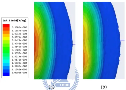
3.1.6 SAR distribution (t=15 ns) in the yz section of the muscle cubic (a)
SAR distribution without metamaterials (b) SAR distribution with
metamaterials ...24
3.1.7 SAR distribution with HFSS solver (a) SAR distribution without
metamaterials (b) SAR distribution without metamaterials. ...25
3.1.8 The head and antenna models for SAR calculation...26
3.1.9 Calculated SAR
1gfrom FDTD simulation...26
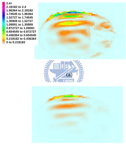
3.1.11 SAR values in the horizontal cross section of this head (a) without
metamaterials (b) with metamaterials...28
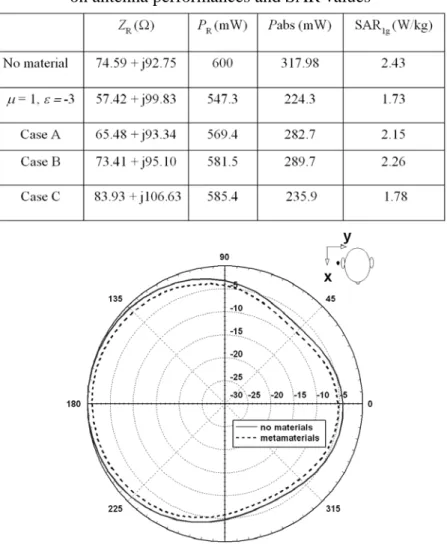
3.1.12 Calculated
φlane radiation pattern at 900 MHz ...29
3.2.1 The structures of split ring resonators (SRRs)...31
3.2.2 Top view of the FDTD setup for SRRs simulation (
H||)...32
3.2.3 Modeled transmission spectra of SRRs placed in the yz plane ...32
3.2.4 Top view of FDTD simulation for SRRs placed in the xz plane (
H⊥) ...33
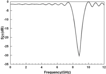
3.2.5 Modeled transmission spectra of SRRs placed in the xz plane ...33
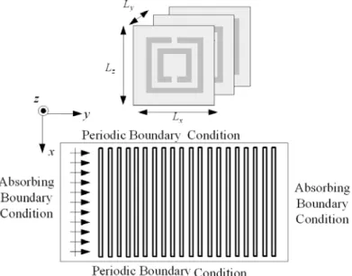
3.2.6 Top view of FDTD simulation for SRRs with dielectric cube ...34
3.2.7 Modeled transmission spectra of SRRs placed in the xz plane with
dielectric cube ...34
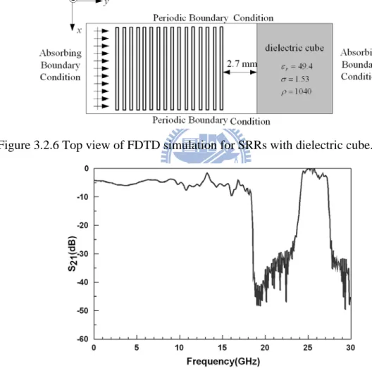
3.2.8 Modeled transmission spectra of the designed SRRs...35
3.2.9 Structure used in SAR calculation...36
4.1.1 The maximum eigenvalues for different propagation direction ...43
4.1.2 Transmission characteristics for power plane study. ... 44
4.1.3 Numerical simulation of the ADI-FDTD with Mur’s ABC (CFLN=3)
...45
4.1.4 Numerical simulation of the ADI-FDTD with Mur’s ABC (CFLN=5)
...45
4.2.1 Four positions for eigenvalue calculation...50
4.2.2 Conductivity profiles for the PML mediums...52
4.2.3a Relative reflection error of the TM ADI-FDTD method with PML
ABC ...54
4.2.3b Relative reflection error of the TE ADI-FDTD method with PML
ABC ...55
4.2.4 The H
xcomponent with the conventional conductivity profile...56
4.2.5 The H
xcomponent with the modified PML conductivity profile...56
4.5.1 The H
xcomponent for ADI-FDTD with unsplit-field PML
(CFLN=2) ...64
4.5.2 The H
xcomponent for ADI-FDTD with split-field PML (CFLN=7)...65
4.6.1 Multilevel crossover in VLSI interconnect...66
4.6.2 Voltage at Port 1 with the conventional PML conductivity profile ...67
4.6.3 Voltage at Port 1 with the modified PML conductivity profile ...67
4.6.4 Voltages at different ports of the multilevel crossover ...68
4.6.5 Cross section view and layout of the spiral inductor with h
3-h
5= 1.3
um, h
2= 3.6 um, h
1= 200 um, h
4= 2.07 um, and h
5= 0.84 um...69
4.6.6 Measured and simulated Q-factor...70
5.1.1 Geometry of two PIFAs using coupling element for isolation
enhancement ...73
5.2.1 Equivalent circuit model of the coupling element... 74
5.2.2 Simulated S parameters for equivalent circuit model
....75
5.2.3. (a) Proposed design for isolation bandwidth enhancement. (b)
Simulated S parameters for the proposed design
....76
5.2.4 Parametric study of the coupling element
....77
5.3.1 Measured S parameters for the reference antenna elements.
....78
5.3.2 Simulated and measured S parameters of the proposed design with
isolation enhancement
..
....78
List of Tables
3.1 electric properties for human head model ... 22
3.2 Comparisons of peak SAR... 26
3.3 Effects of metamaterials on antenna performances and SAR reduction
at 900 MHz ... 27
3.4 Effects of sizes and positions of metamaterials on antenna
performances and SAR values... 29
3.5 Comparisons of SAR reduction techniques with different materials ... 30
3.6 Effect of metamaterials on SAR reduction (P
R= 0.6 W for 900 MHZ)... 30
3.7 Effects of SRRs on the antenna performance and SAR reduction ... 37
3.8 Effect of SAR reduction for 900MHz and 1800MHz bands (P
R= 0.6
W for 900 MHZ AND P
R= 0.125 W for 1800 MHZ)... 37
3.9 Effects of SAR reduction on 5% frequency band for 900MHz and
1800MHz ... 37
4.1 Calculated resonant frequency for different schemes ...44
4.2 Eigenvalues of Λ for free space and PML mediums
σ
=
σ
max...49
4.3
Eigenvalues of Λ for 2D ADI-FDTD with PML ...50
4.4 The calculated eigenvalues of Λ for different conductivity profiles ....53
4.5 Eigenvalues of for Λ and G unsplit PML scheme ...62
4.6 Eigenvalues of Λ and G for split PML scheme ...63
4.7 Multilevel crossover simulation ...68
Chapter 1
Introduction
1.1 SAR Reduction with Metamaterials
The use of the cellular phones has been growing rapidly in the global communities. The absorption of EM energy emitted from cellular phone has been discussed in recent years. Exposure guidelines for protecting the human body from EM exposure have been issued in many countries. More and more people concern the absorption of electromagnetic radiation from cellular phone in the human head.
Figure 1.1.1 The SAR distribution in the human head
The specific absorption rate (SAR) is a defined parameter for evaluating power deposition in human tissue, as shown in Fig. 1.1.1. For the cellular phone compliance, the SAR value must not exceed the exposure guidelines [1, 2]. Some numerical results
have implied that the peak 1 g averaged SAR value (SAR1g) may exceed the exposure
guidelines when a portable telephone is placed extremely close to the head [3, 4]. Therefore, many researchers are working on reducing the SAR values. In [5], a ferrite sheet was proposed to use as a protection attachment between the antenna and a head. It was found that a ferrite sheet can result in SAR reduction and the radiation pattern of the antenna can be less affected. In [6], a PEC reflector was arranged between a human head and the driver of a folded loop antenna. Numerical results showed that the radiation efficiency can be enhanced and the peak SAR value can be reduced. In [7], a study on the effects of attaching conductive materials to cellular phone for SAR reduction has been presented. It indicated that the position of the shielding material is
an important factor for SAR reduction effectiveness.
Recently, metamaterials have inspired great interests due to their unique physical properties and novel application [8, 9]. Metamaterials denote artificially constructed materials having electromagnetic properties not generally found in nature. Two important parameters, electric permittivity and magnetic permeability determine the response of the materials to the electromagnetic propagation. Mediums with negative permittivity can be obtained by arranging the metallic thin wires periodically [10]. On the other hand, an array of split ring resonators (SRRs) can exhibit negative effective permeability [11]. The metallic thin wires and split ring resonators are narrow-banded and lossy materials, as shown in Fig. 1.1.2.
x L z L y L
w
l
r 2 c d g l (a) (b)Figure 1.1.2 (a) thin wire structure (b) split-ring resonator (SRR).
When one of the effective medium parameters is negative and the other is positive, the medium will display a stop band. The metamaterials is on a scale less than the wavelength of radiation and uses low density of metal. The structures are resonant due to internal capacitance and inductance. The stop band of metamaterials can be designed at operation bands of cellular phone while the size of metamaterials is similar to that of cellular phone. In [12], the designed SRRs operated at 1.8 GHz were
used to reduce the SAR value in a lossy material.The metamaterials are designed on
circuit board so it may be easily integrated to the cellular phone. Simulation of wave propagation into metamaterials was proposed in [13]. The authors developed the FDTD method with lossy Drude models for metamaterials simulation. This method is a useful approach to study the wave propagation characteristics of metamaterials [14] and has been further developed with the perfectly matched layer and extended to three-dimension problem [15].
In this work, we will use metamaterials for SAR reduction. An anatomically based human head model and a dipole antenna are assumed. The metamaterials are placed between the antenna and a human head. Preliminary study of SAR reduction with
metamaterials is performed by 3-D FDTD method with lossy Drude model. In order to study SAR reduction of antenna operated at the GSM 900 band, the effective medium parameter of metamaterials is set to be negative at 900 MHz. Different positions, sizes, and negative medium parameters of metamaterials for SAR reduction effectiveness are also analyzed. To investigate the influence of metamaterials on the
antenna, the peak SAR1g and antenna performances are demonstrated. The use of
metamaterials is also compared with other SAR reduction techniques. We design the metamaterials from periodically arrangement of split ring resonators (SRRs). By properly designing structure parameters of SRRs, the effective medium parameter can be negative around 900 MHz and 1800 MHz bands. The SAR value in a simplified muscle cube with the presence of SRRs is studied. Numerical results are demonstrated to validate the effect of SAR reduction with metamaterials.
1.2 Stability Analysis of Absorbing Boundary Conditions for
ADI-FFDTD
Finite-Difference Time-Domain (FDTD) method has been widely used to analyze the electromagnetic problems [16, 17]. Due to the explicit nature of this method, the time step size is restricted by the Courant, Friedrichs, and Lewy (CFL) stability condition. Recently, a stable alternating direction implicit (ADI) scheme was introduced for the FDTD method. The ADI-FDTD method is an attractive method due to its unconditionally stability with large CFL number [18-21]. The flowchart of ADI-FDTD is shown in Fig. 1.2.1.
Update Ex implicitly(with current source) along y direction Update Ey implicitly(with current source)
along z direction Update Ez implicitly(with current source)
along x direction
Update Hx, Hy, Hz explicitly
Update magnetic source
t=t+Δt/2
Update Ex implicitly(with current source) along z direction Update Ey implicitly(with current source)
along x direction Update Ez implicitly(with current source)
along y direction
Update Hx, Hy, Hz explicitly
Update magnetic source
t=t+Δt/2
When the ADI-FDTD method is used to simulate unbounded region problems, efficient absorbing boundary conditions (ABCs) must be employed. The commonly used ABCs are Mur’s first order ABC and perfectly matched layer (PML) medium. In [22, 23], the Mur’s first order ABC was implemented in the ADI-FDTD method to simulate microstrip circuits. A split field PML [24] was employed for the ADI-FDTD method [25, 26]. However, the implementation of ABCs in the ADI-FDTD method can affect the stability of this scheme. For analytical ABCs, it is found that the implementation of the third order Higdon’s ABC in the ADI-FDTD method will cause instability in the simulation results [27]. In [28, 29], it is found that the ADI-FDTD method with split-field PML will lead to late-time instability from numerical simulations. In [28], the authors indicate that the instability from the split-field PML equations can be prevented by using an unsplit form PML implementation. However, the split-field PML formulation is less complicated and more straightforward compared to the unsplit form PML implementation. Therefore, a more stable PML implementation for ADI-FDTD method is highly desirable.
It is important to analyze the stability of the absorbing boundary condition for the ADI-FDTD method. In this work, first, the stability analysis of the Mur’s first order ABC in the ADI-FDTD method is demonstrated. The theoretical stability analysis of this scheme also is studied by deriving the amplification matrix. The effect of the wave propagation direction on the stability of this scheme is investigated. From the stability analysis, it is found that the ADI scheme of the Mur’s first order ABC is unstable. Since we focus on analyzing the stability of the Murs’ ABC at the boundary and do not consider the stability of the total computation domain, the proposed stability analysis is approximate. The stability analysis of the total computational domain can be accomplished by numerical simulation with a large number of time steps. In this work, the numerical tests of the ADI-FDTD method with Mur’s ABC are performed. Numerical results of this scheme with different time step size will be demonstrated to validate the instability of this scheme.
Then, the theoretical stability analysis of the ADI-FDTD method with split-field PML will be studied through deriving the amplification matrix. The amplification matrix is derived using the actual updating equations of the field components. From the stability analysis, it is found that this scheme will be unstable at the PML interface and inside the PML regions. The effect of the PML conductivity profile on the stability of this scheme will be investigated [30]. We find that the instability of this scheme is due to the conductivities within the PML medium. The instability of this scheme inside the PML regions can be improved significantly with the modified PML conductivity profile. Numerical results of the 3-D ADI-FDTD method with split-field PML will be demonstrated to validate the theoretical results.
The ADI-FDTD method is an attractive method since the time step size is not restricted by the CFL condition. Therefore, this method can model the electromagnetic effects of the VLSI circuits efficiently. The frequency domain characteristics of the VLSI circuit can be obtained from the Fourier transform of the transient time domain waveform and it requires a large number of time steps to complete the simulation by FDTD method. This study will be difficult or even impossible due to the late-time instability of ADI-FDTD method with PML absorbing boundary condition. It is not apparent in the literature that anyone has studied the frequency domain characteristics of the VLSI circuits by the ADI-FDTD method with
PML absorbing boundary condition.
The Crank-Nicolson FDTD (CN-FDTD) is found to be another alternative unconditionally stable FDTD method. The ADI-FDTD can be seen as an approximation of the CN-FDTD scheme [31]. In [32, 33], the CN -FDTD with split-field PML and nearly PML (NPML) were proposed. It is shown that the CN-FDTD can remain unconditionally stable with PML implementation. The stability analysis of the PML schemes for the CN-FDTD and ADI-FDTD will be studied. The Von Neumann analysis is used to determine the stability of these schemes. The
difference between the CN-FDTD and ADI-FDTD is the Δt2
perturbation term. From this study, it is found that the perturbation term will affect the stability of PML schemes for ADI-FDTD method. This study can provide information to improve the PML scheme for ADI-FDTD method.
In previous study [30], it is found that the PML conductivity profile will affect the stability of the ADI-FDTD method with Berenger’s PML absorber. The modified PML conductivity profile is employed in this work to investigate the electromagnetic effects of the VLSI circuits in time domain and frequency domain. From the simulation results, it is found that the instability of this scheme can be improved with the modified PML conductivity profiles. Numerical simulations of the VLSI interconnect and RF inductor will be performed to show the efficiency and accuracy of the proposed scheme
1.3. Coupling element for antenna isolation enhancement
The isolation between antennas is a critical parameter in many practical applications such as antenna arrays, diversity antennas and also multiple input multiple output (MIMO) communication systems. However, when antennas are closely packed, strong mutual coupling will degrade radiation patterns and decrease antenna efficiency, which will cause deterioration in signal-to-noise ratio and signal to-interference-plus-noise ratio of the systems
create an additional coupling path for enhancing the isolation. The coupling element is placed between antennas and therefore no extra space is needed with this design. This coupling element is not physically connected to the antenna elements and is flexible for controlling the center frequency, bandwidth, and level of isolation. To demonstrate the idea, two antenna elements for using in 2.4 GHz WLAN band are studied. From this study, it is found that the design can achieve more than 15 dB isolation improvement with 5 mm antenna spacing. The detail parametric studies are provided, which show the design of the proposed structure.
1.4 Organization of the Dissertation
This dissertation is organized as follows: First, we will discuss FDTD modeling method and its algorithm in Chapter 2. The FDTD method can use to simulate the metamaterials, calculate the radiation pattern of the antenna affected by the metamaterials, and calculate the SAR values in the human head. In Chapter 3, we will employ the Drude model into FDTD to investigate the effect of the metamaterials on SAR reduction. The design concept of split ring resonators (SRRs) is introduced. With the use of periodical boundary condition and total field / scatter field FDTD schemes, we will design the SRRs to operate at 900MHz and 1800MHz. The SAR reduction with the designed SRRs will be demonstrated. In Chapter 4, the stability analysis of the absorbing boundary conditions (ABCs) for ADI-FDTD will be demonstrated. Theoretical stability analysis and numerical simulation of the split-field PML and Mur’s ABC for ADI-FDTD method will be studied. The modified PML conductivity profile is proposed to improve the stability of the split-field PML scheme for ADI-FDTD. The CN-FDTD can remain stable with PML scheme. The difference between the ADI-FDTD and CN-FDTD is the perturbation term. With this modified PML scheme, the time domain and frequency domain characteristics of VLSI circuits will be investigated. In Chapter 5, a coupling element to enhance the isolation between two closely packed antennas for 2.4 GHz wireless local area network (WLAN) application is introduced. The proposed structure occupies two antenna elements and a coupling element in between. The advantage of this design is that no extra space is needed for antenna elements. The proposed coupling element for antenna isolation will be discussed. Conclusions are drawn in Chapter 6.
Chapter 2
FDTD Method
The finite difference time domain (FDTD) is widely used to simulate the
electromagnetic problems. In this chapter, the basic FDTD algorithm is described. To simulate open region problems, the absorbing boundary condition (ABC) is employed for FDTD method. The commonly used ABCs include Mur’s ABC and perfect matched layer (PML). With the implementation of near field to far field transformation algorithm, the FDTD method can simulate the radiation pattern of the antenna. The modeling of the lumped elements by FDTD method will also be discussed. Finally, the flow of the FDTD computation will be described.
2.1 From Maxwell’s Equations to FDTD Method.
We will derive the 3-D time domain Maxwell’s equations to develop FDTD method. In this study, we consider the source free region with lossy electric and lossy magnetic mediums. To calculate the magnetic loss, the magnetic current density M is defined as
'
M =ρH (2.1.1)
To calculate electric loss, we define the equivalent electric current J
J =σE (2.1.2)
Theρ'
is magnetic resistivity and σ is the electric conductivity. From Maxwell’s
equations, we can obtain
H E t H μ ρ μ ' 1∇× − − = ∂ ∂ (2.1.3) 1 E H E t σ ε ε ∂ = ∇× − ∂ (2.1.4)
2.1.1 Three-dimension Electric and Magnetic Field Equations
Based on the equations (2.1.3) and (2.1.4), we can derive the 3-D electric and magnetic field equations.
⎟⎟ ⎠ ⎞ ⎜⎜ ⎝ ⎛ − ∂ ∂ − ∂ ∂ − = ∂ ∂ x z y x H y E z E t H 1 ρ' μ (2.1.5) ⎟ ⎠ ⎞ ⎜ ⎝ ⎛ − ∂ ∂ − ∂ ∂ − = ∂ ∂ y x z y H z E x E t H 1 ρ' μ (2.1.6) ⎟⎟ ⎠ ⎞ ⎜⎜ ⎝ ⎛ − ∂ ∂ − ∂ ∂ − = ∂ ∂ z y x z H x E y E t H 1 ρ' μ (2.1.7) 1 y x z x H E H E t ε y z σ ∂ ⎛ ⎞ ∂ = ∂ − − ⎜ ⎟ ∂ ⎝ ∂ ∂ ⎠ (2.1.8) 1 y x z y E H H E t ε z x σ ∂ = ⎛∂ −∂ − ⎞ ⎜ ⎟ ∂ ⎝ ∂ ∂ ⎠ (2.1.9) 1 y x z z H H E E t ε x y σ ∂ ⎛ ∂ ⎞ ∂ = − − ⎜ ⎟ ∂ ⎝ ∂ ∂ ⎠ (2.1.10)
The six field partial differential equations form the basic FDTD algorithms.
2.1.2 Finite Difference Method and Yee Algorithm
In this section, we will derive the FDTD method based on Yee algorithm [16]. In Yee algorithm, the derivatives of space and time are expressed by centre difference method. By applying the Yee algorithm for Maxwell’s equations, the FDTD method
can be obtained. To begin the development of FDTD, we consider 1-D lossless condition as an example. x E t Hy z ∂ ∂ = ∂ ∂ μ 1 (2.1.11) According to a derivative definition, (2.1.11) can be written as
x E t H z x y t Δ Δ = Δ Δ → Δ → Δ 0 lim0 1 lim μ (2.1.12) We can note that the exact solution of (2.1.12) is (x, t)
Based on the Maxwell’s equation, the derivatives of time and space in (2.1.12) are discretized by using centre difference expression, therefore we can obtain
(
)
(
)
(
)
(
)
n i t i z i z x n y n y x x x E x x E t t t H t t H Δ Δ − − Δ + = Δ Δ − − Δ + 2 2 1 2 2 μ (2.1.13)The solution of (2.1.13) is (xi, tn) and ( , )x t will be close to (x, t). i n
Based on the FDTD method, the magnetic field ( )
2 y n t H t +Δ can be expressed as
(
)
(
)
[
(
)
(
)
]
n i i t i z i z x n y x n y E x x E x x x t t t H t t H 2 2 +Δ 2 − −Δ 2 Δ Δ + Δ − = Δ + μ (2.1.14)We denote i and n to express the space and time position, respectively. (2.1.14) can be further modified as
[
n]
i n i n i n i E E x t H H +12 −12 +12− −12 Δ Δ + = μ (2.1.15)From (2.1.15), in order to calculate the magnetic fieldHin+1/ 2, we need to obtain the same magnetic field in the earlier time step at the same location and the electric fields located at± Δx/ 2. Similarly, the electric field can be obtained as follow
1 1/ 2 1/ 2 1/ 2 1/ 2 1 n n n n i i i i t E E H H x ε + + + + = + + Δ ⎡Δ ⎣ + − ⎤⎦ (2.1.16)
From (2.1.15) and (2.1.16), the electric and magnetic fields in the FDTD can be obtained from the fields in the earlier time step. The fields in space and time can be expressed as shown in Fig. 2.1.1.
i-1 i-1/2 i i+1/2 i+1 i+3/2 n-1 n-1/2 n n+1/2 n+1 n+3/2 (i,n) /2 t Δ / 2 x Δ 1/ 2 n i E+ 1/2 n i E− 1/ 2 1 n i H++ 1/ 2 n i H+ 1/ 2 n i H− 1 1/ 2 n i E++
Figure 2.1.1 The fields in the space cell.
In (2.1.16), the time and space are variables. From (2.1.16), any 3-D location in the Yee cell can be expressed as
( , , )i j k = Δ(i x j y k z, Δ , Δ (2.1.17) ) Here, Δx, Δy, and Δz are space increment in x, y, and z direction.
We can define the function u in the space and time in the Yee cell as , ,
( , , , ) i j kn
u i x j y k z n zΔ Δ Δ Δ =u (2.1.18) The Δt is time increment and n is an integer.
Based on the Yee algorithm, we can obtain the space derivative of u in the x direction
( , , , ) 1/ 2, , 1/ 2, , [( ) ]2 n n i j k i j k u u u i x j y k z n z O x x x + − − ∂ Δ Δ Δ Δ = + Δ ∂ Δ (2.1.19)
For time consideration, we can obtain the time derivative of u 1/ 2 1/ 2 , , , , 2 ( , , , ) [( ) ] n n i j k i j k u u u i x j y k z n z O t t t + − − ∂ Δ Δ Δ Δ = + Δ ∂ Δ (2.1.20)
In (2.1.19) and (2.1.20), O[(Δx) ]2 and O[(Δt) ]2 are error terms.
From previous study, it is found that the FDTD is based on the Maxwell’s equation.
For example, the field component Hx in space and time can be expressed as
⎟ ⎟ ⎟ ⎟ ⎟ ⎟ ⎟ ⎟ ⎟ ⎠ ⎞ ⎜ ⎜ ⎜ ⎜ ⎜ ⎜ ⎜ ⎜ ⎜ ⎝ ⎛ − Δ − − Δ − = Δ − + − − + − + n k j i x k j i n k j i z n k j i z n k j i y n k j i y k j i n k j i x n k j i x H z E E z E E t H H , , ' , , , 2 / 1 , , 2 / 1 , 2 / 1 , , 2 / 1 , , , , 2 / 1 , , 2 / 1 , , 1 ρ μ (2.1.21)
However, there will be some computational calculation problem for Hx i j k|n, ,
and 1/ 2 , , |n x i j k H + 、 |, ,1/ 2 n x i j k H − . We can rewritten Hx i j k|n, , as
2 2 / 1 , , 2 / 1 , , , , − + + = n k j i x n k j i x n k j i x H H H (2.1.22)
After substituting (2.1.22) into (2.1.21), we can obtain
⎟ ⎟ ⎟ ⎟ ⎟ ⎟ ⎟ ⎟ ⎟ ⎠ ⎞ ⎜ ⎜ ⎜ ⎜ ⎜ ⎜ ⎜ ⎜ ⎜ ⎝ ⎛ + − Δ − − Δ − Δ = − − + − + − + − + 2 2 / 1 , , 2 / 1 , , ' , , , 2 / 1 , , 2 / 1 , 2 / 1 , , 2 / 1 , , , , 2 / 1 , , 2 / 1 , , n k j i x n k j i x k j i n k j i z n k j i z n k j i y n k j i y k j i n k j i x n k j i x H H z E E z E E t H H ρ μ (2.1.23)
(2.1.23) can be further modified as
⎟ ⎟ ⎟ ⎟ ⎟ ⎟ ⎟ ⎠ ⎞ ⎜ ⎜ ⎜ ⎜ ⎜ ⎜ ⎜ ⎝ ⎛ Δ − − Δ − ⎟ ⎟ ⎟ ⎟ ⎟ ⎠ ⎞ ⎜ ⎜ ⎜ ⎜ ⎜ ⎝ ⎛ Δ + Δ + ⎟ ⎟ ⎟ ⎟ ⎟ ⎠ ⎞ ⎜ ⎜ ⎜ ⎜ ⎜ ⎝ ⎛ Δ + Δ − = − + − + + + z E E z E E t t H t t H n k j i z n k j i z n k j i y n k j i y k j i k j i k j i n k j i x k j i k j i k j i k j i n k j i x , 2 / 1 , , 2 / 1 , 2 / 1 , , 2 / 1 , , , , ' , , , , 2 / 1 , , , , ' , , , , ' , , 2 / 1 , , 2 1 2 1 2 1 μ ρ μ μ ρ μ ρ (2.1.24)
The electric fieldsE ,x E and y Ez can be obtained by the same procedure. For
example, the electric fieldEzcan be expressed as , , , , , , , , , , 1 , , 1/ 2 1/ 2 1/ 2, , 1/ 2, , , , 1/ 2 1/ 2 , , , 1/ 2, , 1/ 2, , , 1 2 | 1 2 | | | | | 1 2 i j k i j k n z i j k i j k i j k n z i j k n n y i j k y i j k i j k n n i j k x i j k x i j k i j k t E t E H H t x t H H y σ ε σ ε ε σ σ + + + + − + + + − Δ ⎛ ⎞ − ⎜ ⎟ ⎜ ⎟⋅ Δ ⎜ ⎟ + ⎜ ⎟ ⎜ ⎟ ⎝ ⎠ = ⎛ ⎞ ⎛ Δ ⎞ − ⎜ ⎟ ⎜ ⎟ Δ ⎜ ⎟ ⎜ ⎟ + Δ ⋅⎜ ⎟ ⎜ + ⎟ − − ⎜ ⎟ ⎜ ⎟ ⎜ ⎟ ⎜ Δ ⎟ ⎝ ⎠ ⎝ ⎠ (2.1.25)
We can derive the six field components based on the FDTD method. The field components located in the Yee cell is shown in Fig. 2.1.2. It can be found that the electric field component is surrounded by the magnetic field components and the
magnetic field component is surrounded by the electric field components ( , , ) y H i j k ( , , ) z E i j k ( 1, , ) z E i+ j k ( , , 1) x E i j k+ ( , , ) x E i j k ( , , 1) y E i j k+ ( , 1, 1) x E i j+ k+ ( 1, , 1) y E i+ j k+ ( , , 1) z H i j k+ ( 1, , ) y E i+ j k ( 1, 1, ) Ez i+ j+ k ( 1, , ) x H i+ j k x Δ y Δ z Δ
Figure 2.1.2 The field components in the Yee cell.
2.2 Numerical Stability
In the FDTD method, we need to decide the grid size first. The grid size will affect the numerical dispersion. When the grid size is fixed, the time step size Δt can also be decided based on the stability criterion.
The grid size will depend on the highest operation frequency fu of the modeled
structure. The grid size is usually set to be smaller thanλu /10 to avoid serious
numerical dispersion.
After the grid size is fixed, the time step size Δt can also be calculated. When the wave propagates in one time step, the propagation distance should not be over the grid size. To avoid numerical stability problem, the time step size should meet the FDTD Courant-Friedrich-Levy (CFL) criterion.
( ) ( ) ( )
2 2 2 1 1 1 1 t c x y z Δ ≤ + + Δ Δ Δ (2.2.1)2.3 Material Set
In this research, the material setting for FDTD simulation includes:
A. Metal Structure: The ground plane or the microstrip is metal structure. We usually
assume the metal is perfect electric conductor (PEC). The thickness of metal is set to be very small and the tangential electric field is zero for metal structure.
B. Dielectric structure: The dielectric constant εr is set in FDTD for different
dielectric materials.
constant between two different materials. For example, we usually set the dielectric constant for air is ε0 and dielectric constant for dielectric material is εr.
The dielectric constant of the interface is 0
2 r
ε +ε
.
2.4 Source Condition
For FDTD simulation, the sine wave is usually used with operation frequency f . 0
The expression for sine wave is
0 0
( ) sin(2 )
f t =E π f n tΔ (2.4.1)
In our simulation, the Gaussian source is commonly used. We can set the source that is centered at time step n and has a 1/e characteristic decay of 0 ndecay time steps, the Gaussian source can be expressed as
0 [( ) / ] 0
( ) n n ndecay
f t =E e− − (2.4.2) In the FDTD simulation, we set the source for electric field directly. For example, if we set the source at i for Es z component, it can be written as
0 0 | ( ) sin(2 ) S n z i E = f t =E πf n tΔ (2.4.3)
2.5 Absorbing Boundary Condition
In the FDTD method, the absorbing boundary condition (ABC) is used to simulate open region problem. As shown in Fig 2.5.1, the electric field components at the boundaries should meet a particular condition to avoid reflection wave from the boundary. 1 i= i=imax max j= j 1 j= lattice boundary radiated wave source
Figure 2.5.1 Absorbing boundary condition for FDTD method.
condition [34] and perfectly matched layer (PML) [24]. They are discussed briefly.
2.5.1 Mur’s ABC
There are two types Mur’s ABCs including Mur’s first order ABC and Mur’s
second order ABC. We consider the electric field component Ezin a 2-D space at
x= Δi xand y= Δ . For Mur’s first order ABC,j y Ez can be expressed as
(
)
1 1 , 1, 1, , n n n n i j i j i j i j c t x E E E E c t x + + − − Δ − Δ = + − Δ + Δ (2.5.1)If we assume xΔ = Δ , the Mur’s second order ABC in 2-D domain can be expressed y
as
(
)
(
)
( )
1 1, 1, , 1, , 1 2 , , 1 , , 1 1, 1 1, 1, 1 2 ( 2 2 ) 2( )( ) n n n n n i j i j i j i j i j n i j n n n n n n i j i j i j i j i j i j c t x x E E E E E c t x c t x E c t E E E E E E x c t x + − − − + + − − + − − − Δ − Δ Δ − + − + + Δ + Δ Δ + Δ = Δ + − + + − + Δ Δ + Δ (2.5.2)In the Mur’s first order ABC, the field componentEzatx= Δi x is calculated from
z
E at x= Δi x at earlier time step and the field componentEz atx= − Δ at the (i 1) x current time step. The Mur’s ABC is simple and easy to implement.
2.5.2 Perfectly Matched Layer (PML)
The Berenger proposed the PML absorbing boundary condition in 1994 [24]. By using the electric and magnetic conductivities, the reflection wave can be minimized inside the PML medium. The PML medium can absorb the propagation wave in any direction. When using the PML, we need to split the electric and magnetic field
components. For TM wave, the field components Ezx and Hx in the PML can be
expressed as ⎟ ⎟ ⎠ ⎞ ⎜ ⎜ ⎝ ⎛ Δ − ⎟ ⎟ ⎟ ⎟ ⎠ ⎞ ⎜ ⎜ ⎜ ⎜ ⎝ ⎛ Δ + Δ + ⎟ ⎟ ⎟ ⎟ ⎠ ⎞ ⎜ ⎜ ⎜ ⎜ ⎝ ⎛ Δ + Δ − = + − + + + x H H t t E t t E n j i y n j i y x n j i zx x x n j i zx 2 / 1 , 2 / 1 2 / 1 , 2 / 1 , 1 , | | 2 1 | 2 1 2 1 | ε σε ε σ ε σ (2.5.3) ⎟ ⎟ ⎠ ⎞ ⎜ ⎜ ⎝ ⎛ Δ − − ⎟⎟ ⎟ ⎟ ⎟ ⎠ ⎞ ⎜⎜ ⎜ ⎜ ⎜ ⎝ ⎛ Δ + Δ + ⎟⎟ ⎟ ⎟ ⎟ ⎠ ⎞ ⎜⎜ ⎜ ⎜ ⎜ ⎝ ⎛ Δ + Δ − = − + − + y E E t t H t t H n j i z n j i z y n j i x y y n j i x 2 / 1 , 2 / 1 , * 2 / 1 , * * 2 / 1 , | | 2 1 | 2 1 2 1 | μ σ μ μ σ μ σ (2.5.4)
Theσxandσ*xare electric conductivity and magnetic conductivity, respectively. They
conductivity in the PML medium. Wave source * 1 1 (0,0, y, y) PML σ σ * 2 2 (0,0, y, y) PML σ σ * 2 2, ( x, x ,0,0) PMLσ σ * 1 1, ( x, x , 0, 0) PMLσ σ * * 1 1, 2 2, ( x, x , y , y ) PMLσ σ σ σ * * 2 2, 2 2, ( x , x , y , y ) PMLσ σ σ σ * * 1 1, 1 1, ( x, x , y, y ) PMLσ σ σ σ PML(σ σx2, *x2,,σ σy1, y*1,) outgoing wave perfect conductor
Figure 2.5.2 PML absorbing boundary condition
The PML impedance can be matched to the free space impedance with the condition μ
σ ε
σ *
= (2.5.5) The PML conductivity profile is usually scaled to reduce the reflection error.
s m opt s Δ + ≈ = π σ σ 150 ) 1 ( max m m s s d s s s) max 0 ( =σ − σ s = x, y, z (2.5.6)
where d is the thickness of PML absorber, Δs is the cell size, and s0 represents the
interface. Typically, we choose m = 4 for optimum PML performance [25]
2.6 Near Field to Far Field Transformation
It is not practical to directly simulate the electric and magnetic fields in the far field within the FDTD grid. This will require a large computational domain to include the far field. The field components in the far field can be calculated by near field to far field transformation [35]. First, we calculate the equivalent electric current and equivalent magnetic current in the near field in the region enclosed the computational domain. From the near field equivalent electric current and equivalent magnetic current, we can obtain the field components in the far field. We can calculate the antenna radiation pattern by using this method.
As shown in Fig 2.6.1, we use the virtual surface S to enclose the B region. First ab
we can calculate the tangential fieldsE ands H . After obtaining thes E ands H , we can s
calculate the equivalent surface electric current J and equivalent surface magnetic s
J rs( )= ×n H rˆ s( ) (2.6.1) ˆ
( ) s( )
s
M r = − ×n E r (2.6.2) where nˆ is normal to the surface of Sab
Grid boundary(ABC)
Near to far field transformation boundary ˆ S S J = ×n H ˆ S S M = ×n E ab S , s s H E ˆ n 1 cells B A
Figure 2.6.1 Near field to far field transformation
In the near field to far field transformation, the near field in the closed volume is calculated first. Then, the field components in the far field can be calculated by Kirchhoff surface integral representation (KSIR) as
( )
( )
( )
( )
' ' ' ' ' 2 ' ' 3 ' ' , , , ' ˆ 4 1 , da dt t r cR R t r R R R t r n t r s∫
⎥ ⎦ ⎤ ⎢ ⎣ ⎡∇ − − ∂ = r r r r r r ψ ψ ψ π ψ (2.6.3) whererris any point in the far field '
rris the point at the surface of the FDTD computational domain
'
Rr r r= −r r
| |
R= Rr
ˆ
nis normal to the computational surface
c is light velocity '
a is closed surface for FDTD method
The KSIR can calculate the field components in the far field outside the computational domain. Therefore, we can calculate the field components in the far field as follow
A. The near field components of arbitrary scatter can be calculated by FDTD method easily.
B. The far field components in any direction can be calculated from the KSIR method.
in the far field. The frequency domain field components can be obtained by using Discrete Fourier Transformation (DFT) method.
2.7 Lumped Elements
FDTD method can also be used to simulate linear and non-linear lumped elements [36, 37]. We assume the lumped elements are place in the z-direction, and the FDTD method for lumped elements is described as follow
2.7.1 FDTD Method for Lumped Elements
We consider the Maxwell’s equation with current source c D H J t ∂ ∇× = + ∂ r r r (2.7.1) where Jc =σE r r
andDr =εEr , we can discretized the (2.7.1) by central difference
method 1/ 2 1/ 2 , , 1/ 2, , 1/ 2, , , , , , 1 , , , , 1/ 2 1/ 2 , , , , , 1/ 2, , 1/ 2, , , , , | | 1 2 | | | | 1 1 2 2 n n i j k y i j k y i j k i j k i j k n n z i j k z i j k n n i j k i j k x i j k x i j k i j k i j k t t H H x E E t t H H y σ ε ε σ σ ε ε + + + − + + + − + Δ ⎛ ⎞ ⎛ − ⎞ ⎛ Δ ⎞ − ⎜ ⎟ ⎜ ⎟ ⎜ ⎟ Δ ⎜ ⎟ ⎜ ⎟ ⎜ ⎟ = Δ + Δ ⎜ ⎟ ⎜ + ⎟ ⎜ + ⎟ − ⎜ ⎟ ⎜ ⎟ ⎜ ⎟ ⎜ ⎟ ⎜ ⎟⎜ Δ ⎟ ⎝ ⎠ ⎝ ⎠⎝ ⎠ (2.7.2)
It should be noticed that the magnetic field is at (n+1/2) time step, which is located between theEz i j k|n, , andEz i j k|n, ,+1 . TheJcis also at the time step (n+1/2)th time step and can be calculated by
(
)
, , 1/ 2 1/ 2 1 , , , , , , , , , , | | | | 2 i j k n n n n c i j k i j k z i j k z i j k z i j k J + =σ E + =σ E +E + (2.7.3)We assume all the lumped elements are in free space (ε = ε0, σ = 0, and Jc = 0). The
H
∇× for FDTD can be rewritten as
1/ 2 1/ 2 1/ 2 1/ 2 1/ 2, , 1/ 2, , , 1/ 2, , 1/ 2, 1/ 2 , , |n |n |n |n y i j k y i j k x i j k x i j k n i j k H H H H H x y + + + + + − − + + − − ∇× = + Δ Δ (2.7.4)
Therefore, (2.7.2) can become
1 1/ 2 , , , , , , 0 |n |n n z i j k z i j k i j k t E E H ε + = +Δ ∇× + (2.7.5)
In the FDTD method, we will introduce the current densityJLfor lumped elements
C L D H J J t ∂ ∇× = + + ∂ r r r r (2.7.6) Assuming the element located at Ez i j k|, , in the z direction. The relation between the
current density JLand lumped element current ILis L L I J x y = Δ Δ (2.7.7) , , | z i j k V =E Δz (2.7.8) From (2.7.5), the FDTD algorithm for lumped element can be written as
, ,1 , , , ,1/ 2 1/ 2 0 0 |n |n n n z i j k z i j k i j k L t t E E H I x y ε ε + = +Δ ∇× + − Δ + Δ Δ (2.7.9) 2.7.2 Resistor
We assume to place a resistor at Ez i j k|, , in the z direction. The relation for voltage and current is |, ,1/ 2
(
|, ,1 |, ,)
2 n n n z i j k z i j k z i j k z I E E R + = Δ + + 1/ 2 , , |n z i j k L I J x y + = Δ Δ (2.7.10) Substituting the (2.7.10) into (2.7.9), we can obtain the FDTD algorithm for resistor.1 0 0 1/ 2 , , , , , , 0 0 1 2 | | 1 1 2 2 n n n z i j k z i j k i j k t z t R x y E E H t z t z R x y R x y ε ε ε ε + + Δ Δ Δ ⎛ − ⎞ ⎛ ⎞ ⎜ Δ Δ ⎟ ⎜ ⎟ ⎜ ⎟ ⎜ ⎟ = + ∇× Δ Δ Δ Δ ⎜ + ⎟ ⎜ + ⎟ ⎜ Δ Δ ⎟ ⎜ Δ Δ ⎟ ⎝ ⎠ ⎝ ⎠ (2.7.11)
2.7.3 Resistive Voltage Source
The FDTD can also simulate the resistive voltage source. We assume the element is placed in z direction and the relation between the voltage and current is
(
)
1/ 2 1/ 2 1 , , , , , , | | | 2 n n n n S z i j k z i j k z i j k S S V z I E E R R + + = Δ + + + 1/ 2 , , |n z i j k L I J x y + = Δ Δ (2.7.12) where VSn+1/ 2is excitation source andR is matching impedance SThe FDTD algorithm for resistive voltage source is
1 0 0 1/ 2 0 1/ 2 , , , , , , 0 0 0 1 2 | | 1 1 1 2 2 2 n n n S n z i j k z i j k i j k S S t z t t R x y R x y E E H V t z t z t z R x y R x y R x y ε ε ε ε ε ε + + + Δ Δ Δ Δ ⎛ − ⎞ ⎛ ⎞ ⎛ ⎞ ⎜ Δ Δ ⎟ ⎜ ⎟ ⎜ Δ Δ ⎟ ⎜ ⎟ ⎜ ⎟ ⎜ ⎟ = Δ Δ + Δ Δ ∇× + Δ Δ ⎜ + ⎟ ⎜ + ⎟ ⎜ + ⎟ ⎜ Δ Δ ⎟ ⎜ Δ Δ ⎟ ⎜ Δ Δ ⎟ ⎝ ⎠ ⎝ ⎠ ⎝ ⎠ (2.7.13)
2.8 FDTD Method for Computer Calculation
calculate the electric and magnetic fields in each time step. Before running the FDTD for each time step, we need to set the FDTD parameters like grid size, time step size, source condition. The flow of FDTD method for computation is explained below
2.8.1 Pre-Processing
A. Define the FDTD grid size
B. Define the time step size to meet the stability condition C. Calculate the FDTD parameters for different materials 2.8.2 Time Stepping
A. Assign the excitation
B. Calculate the electric field components
C. Employ the absorbing boundary condition to absorb the outgoing wave. D. Calculate the magnetic field components
2.8.3 Post-Processing
A. Recording the electric and magnetic fields at each time step. B. Calculate the electric and magnetic fields in far field.
Chapter 3
Study of SAR Reduction with
Metamaterials
In this work, the EM interaction between the antenna and the human head is reduced with metamaterials. Preliminary study of SAR reduction with metamaterials is performed by FDTD method with lossy Drude model. It is found that the specific absorption rate (SAR) in the head can be reduced by placing the metamaterials
between the antenna and the head. The antenna performances and radiation pattern
with metamaterials are analyzed. A comparative study with other SAR reduction techniques is also provided. The metamaterials can be obtained by arranging split ring resonators (SRRs) periodically. In this research, we design the SRRs operated at 900 MHz and 1800 MHz bands. The design procedure will be described. Numerical results of the SAR values in a muscle cube with the presence of SRRs are shown to validate the effect of SAR reduction. These results can provide helpful information in designing the mobile communication equipments for safety compliance.
3.1 Preliminary Studies of SAR Reduction by FDTD Method with
Lossy Drude Model
3.1.1 FDTD Method with Lossy Drude Model
Preliminary studies of SAR reduction with metamaterials were performed by FDTD with lossy Drude model. The SAR reduction effectiveness and antenna performance with different positions, sizes, and negative medium parameters of metamaterials will be analyzed. The head model used in this study was obtained from Magnetic resonance imaging (MRI) based head model through The Whole Brain
Atlas website. In the MRI human head model, different colors of the human head
represent different tissues, as shown in Fig. 3.1.1. In this study, six types of tissues, i.e., bone, brain, muscle, eyeball, fat, and skin, were involved in this model.
Figure 3.1.1 MRI human head model
The MRI human head model is discretized for FDTD simulation. Fig. 3.1.2 shows a horizontal cross section through the eyes of this head model. The electrical properties of tissues were taken from [3, 4], as shown in Table 3.1.
Table 3.1 electric properties for human head model 900MHz 1.8GHz Tissue ρ εr σ εr σ Bone 1810 17.4 0.19 15.5 0.39 Brain 1040 44.1 0.89 42.2 1.18 Muscle 1040 51.8 1.11 49.4 1.53 Eyeball 1010 74.3 1.97 73.7 2.33 Fat 920 10.0 0.17 9.55 0.22 Skin 1010 39.5 0.69 38.9 0.95
The formulation of SAR is defined as σ 2ρ
2
E
SAR= , where E, σ, and ρ are the
electric field, conductivity, and mass density in the head, respectively.
Simulations of metamaterials are performed by FDTD method with lossy Drude model [13]. The method is a useful method to understand the wave propagation
characteristics of metamaterials. In this method, let μ and ε be modeled by the
following expressions ⎟⎟ ⎠ ⎞ ⎜ ⎜ ⎝ ⎛ Γ + − = ) ( 1 2 0 e pe i
ω
ω
ω
ε
ε
(3.1.1) ⎟ ⎟ ⎠ ⎞ ⎜ ⎜ ⎝ ⎛ Γ + − = ) ( 1 2 0 m pm i ω ω ω μ μ , (3.1.2)where ωp and Γ denote the corresponding plasma and damping frequencies,
respectively.
We can provide a slight variation of (3.1.1) as
⎟⎟ ⎠ ⎞ ⎜ ⎜ ⎝ ⎛ Γ + Γ + − = ) )( ( 1 1 1 2 0 e e pe i i
ω
ω
ω
ε
ε
(3.1.3)This model is actually Lorentz medium model, e.g.,
⎟ ⎟ ⎠ ⎞ ⎜ ⎜ ⎝ ⎛ − Γ + − = 2 0 2 2 0 1 e e pe L i ω ω ω ω ε ε , (3.1.4) where Γe=Γe1+Γe2and 1 2 2 0e=ΓeΓe ω .
With this method, we can treat the metamaterials as homogenous materials with frequency-dispersive material parameters.
3.1.2 SAR Calculation Verification
The developed FDTD method for SAR calculation is studied and verified. Fig.
3.1.3 shows the muscle cube and antenna models in this study. The antenna was arranged parallel to the cube axis. The muscle cube was formed by muscle tissue with εr = 51.8, σ = 1.11 , and ρ = 1040 at 900 MHz.
Fig. 3.1.3 Test Structure used in SAR calculation.
0 4 8 12 16 20 Time(ns) 0 1 2 3 4 5 6 7 8 S A R (W /K g )
SAR(27 averaged fields) SAR(48 averaged fields)
0 4 8 12 16 20 Time(ns) 0 1 2 3 4 5 6 7 S A R (W /K g ) SAR(dt=9ps) SAR(dt=4.5ps)
(a) different sampled fields (b) different grid size and time step Fig. 3.1.4 SAR calculation in the muscle cubic for numerical tests.
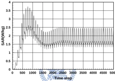
The SAR value was calculated for an antenna output power equal to 1 W. In this FDTD simulation, the Δx =5mm, Δy=5mm, Δz=5mm, and Δt=9.0 ps were used. The
calculated steady-state SAR1g value is shown in Fig. 3.1.4. First, the peak SAR value
was calculated from 27 averaged electric fields. It is found that the calculated peak
SAR1g without metamaterials was 3.70 W/kg. Then, 48 electric fields were averaged
to obtain the SAR values. The calculated peak SAR1g was 3.87 W/kg. Similar results
can be obtained for SAR calculation with different sampled electric fields.
Since the grid size will affect the accuracy of the FDTD simulation, the calculated SAR values for different grid size and time step were studied. The smaller grid size
with Δx =2.5mm, Δy=2.5mm, Δz=2.5mm, and Δt=4.5 ps were also studied. The