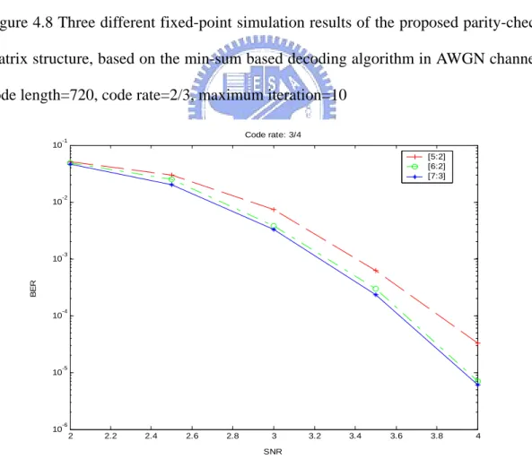
低密度對偶檢查碼結構之改進以及其解碼器之超大型積體電路實現

全文

(1)國立交通大學電子工程學系電子研究所碩士班碩士論文. 低密度對偶檢查碼結構之改進以及其解碼器之超大型積體電路實現. An Improved LDPC Code Structure and Its VLSI Decoder Realization. 研究生：朱元志指導教授：陳紹基博士. 中華民國九十四年七月.

(2) 低密度對偶檢查碼結構之改進以及其解碼器之超大型積體電路實現 An Improved LDPC Code Structure and Its VLSI Decoder Realization 研究生：朱元志. Student：Yuan-Jih Chu. 指導教授：陳紹基博士. Advisor：Sau-Gee Chen. 國立交通大學電子工程學系. 電子研究所所碩士班. 碩士論文 A Thesis Submitted to Institute of Electronics College of Electrical Engineering and Computer Science National Chiao Tung University in Partial Fulfillment of the Requirements for the Degree of Master of Science in Electronics Engineering. July 2005 Hsinchu, Taiwan, Republic of China. 中華民國九十四年七月.

(3) 低密度對偶檢查碼結構之改進以及其解碼器之超大型積體電路實現學生：朱元志. 指導教授：陳紹基博士. 國立交通大學. 電子工程學系電子研究所碩士班. 摘. 要. 由於低密度對偶檢查碼 (LDPC) 的編碼增益接近向農 (Shannon) 極限以及解碼程序上擁有低複雜度的特性，所以在近年來受到廣泛的討論。本文中，我們利用差分集合 (difference family) 的概念來建構一種新的低密度對偶檢查碼結構，此結構在編碼上擁有低複雜度的特性，以及在解碼器的設計上易於超大型積體電路 (VLSI) 實現。此外，在解碼器的設計上，我們使用部分平行 (semi-parallel) 的架構並使其平行度為 10，設計一個碼率為 3/4、長度為 960 位元、最大循環解碼次數為 10 的非規則低密度對偶檢查碼解碼器，在 0.18 µm 製程下，此解碼器之資料流為每秒 370MHz、面積為 80 萬個邏輯閘、消耗功率為 550mW。. I.

(4) An Improved LDPC Code Structure and Its VLSI Decoder Realization Student: Yuan-Jih Chu. Advisor: Dr. Sau-Gee Chen. Department of Electronics Engineering & Institute of Electronics National Chiao Tung University. ABSTRACT In recent years, low-density parity-check (LDPC) codes have attracted a lot of attention due to the near Shannon limit coding gain when iteratively decoded. In this thesis, we construct a new structure of irregular LDPC codes based on using the difference families. The resulting codes can be encoded with low complexity and are suitable for the VLSI implementation of their decoder. With the semi-parallel architecture and a parallel factor of 10, an irregular LDPC decoder has been implemented, of which the code rate is 3/4, the code length is 960 bits, and the maximum number of decoding iterations is 10, respectively. The irregular LDPC decoder can achieve a data decoding throughput of up to 370Mbps, an area of 800k gate counts, and a power consumption of 550mW using the UMC 0.18 µm ASIC process technology.. II.

(5) 誌謝本篇論文的完成承蒙指導教授陳紹基博士兩年多來的悉心指導教誨，讓我能夠確立研究的方向，給予我多方面的協助，在此至上由衷的感激。其次，感謝曲健全學長以及廖彥欽學姊無私地提供協助，使我受益良多。謝謝實驗室的同學世民、觀易、佳旻、偉廷以及承穎，謝謝你們在課業及生活上給予我許多的幫助。還有實驗室的學弟妹們,謝謝你們帶給我們許多美好的回憶。最後，感謝我的家人在背後支持與鼓勵我，還有在天上的爸爸，因為有你的支持及栽培，我才能順利的完成學業，謹致上無限的敬意與感激。. III.

(6) Contents 中文摘要......................................................................................................................Ⅰ ABSTRACT ...............................................................................................................Ⅱ ACKNOWLEDGEMENT ...........................................................................................Ⅲ CONTENTS.................................................................................................................Ⅳ LIST OF TABLES .......................................................................................................Ⅵ LIST OF FIGURES .....................................................................................................Ⅶ Chapter 1 Introduction................................................................................................1 Chapter 2 Low-Density Parity-Check Code..............................................................3 2.1 Fundamental Concept of LDPC Code ...............................................................3 2.2 Code Construction .............................................................................................7 2.3 Encoding ..........................................................................................................10 2.4 Decoding ..........................................................................................................17 2.4.1 Decoding Procedure in One Iteration .....................................................18 2.4.2 Iterative Decoding Procedure .................................................................23 2.4.3 Efficient Check Node Computation........................................................25 Chapter 3 A New Structure for Low-Density Parity-Check Code Using the Difference Family.....................................................................................33 3.1 The Difference Family .....................................................................................33 3.2 The Proposed Structure of LDPC Code...........................................................35 Chapter 4 Simulation Results ...................................................................................39 4.1 Floating-Point Simulations ..............................................................................42 4.2 Fixed-Point Simulations...................................................................................46 4.2.1 Quantization of Initially Received Signal...............................................46 4.2.2 Quantization of rm ,l and q m,l .................................................................50 4.2.3 Summary of Fixed-Point Simulation Results .........................................54 Chapter 5 VLSI Implementation of LDPC Decoder ..............................................56 5.1 Semi-parallel Decoder Architecture for the Proposed LDPC Codes ...............56 5.2 Architectures of the Check Node Function Unit and the Variable Node Function Unit ...................................................................................................59. IV.

(7) Chapter 6 Conclusion ................................................................................................76 References ...................................................................................................................78 Autobiography............................................................................................................81. V.

(8) List of Tables. (. ). Table 2.1. Efficient computation step of p1T = −γ −1 − ET −1 A + C s T .................14. Table 2.2. Efficient computation step of p 2T = −T −1 ( As T + Bp1T ) ......................14. Table 2.3. Summary of Richardson’s encoding procedure. ..................................14. Table 2.4. Summary of the sum-product algorithm ..............................................29. Table 2.5. Summary of the min-sum based algorithm..........................................30. Table 2.6. Summary of the min-sum algorithm ....................................................31. Table 4.1. Polynomials of each of the circulant matrices of the proposed irregular LDPC codes .........................................................................................40. Table 4.2. Polynomials of each of the circulant matrices of the quasi-cyclic irregular LDPC codes ..........................................................................41. Table 5.1. Area, speed, latency and power consumption of the reformulated CNFUs and VNFUs architectures for the sum-product algorithm ......70. Table 5.2. Area, speed, latency and power consumption of the re-mapped CNFUs and VNFUs architectures for the sum-product algorithm....................70. Table 5.3. Area, speed, latency and power consumption of the CNFUs and VNFUs architectures for the min-sum based algorithm ......................71. Table 5.4. Summary of comparison the area, speed and power consumption of the different CNFUs and CNFUs architectures for the sum-product algorithm and the min-sum based algorithm .......................................71. Table 5.5. Summary of the proposed LDPC decoder ...........................................74. Table 5.6. Comparison of LDPC decoders ...........................................................74. Table 5.7. Basic MCS set of TGnSync proposal ..................................................75. VI.

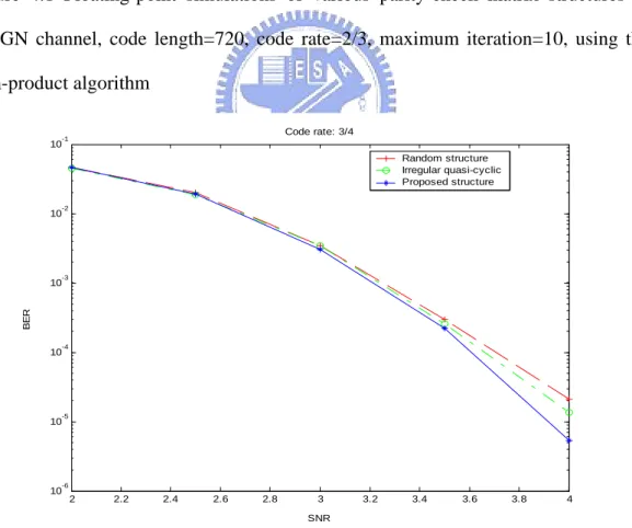
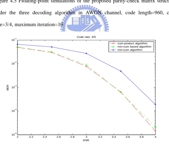
(9) List of Figures Figure 2.1. Example of a (8, 4, 2)-regular LDPC code and its corresponding Tanner graph. There are 8 variable nodes (vi) and 4 check nodes (ci).. .4. Figure 2.2. Example of a low-density parity-check code matrix where (n, j, k) = (20, 3, 4).................................................................................................7. Figure 2.3. Example of a rate-1/2 quasi-cyclic code from two circulant matrices, where a1 ( x) = 1 + x and a 2 ( x) = 1 + x 2 + x 4 ....................................10. Figure 2.4. The parity-check matrix in an approximate lower triangular form......12. Figure 2.5 (a) Example of a rate-1/2 quasi-cyclic code. (a) Parity-check matrix with two circulants, where a1 ( x) = 1 + x and a 2 ( x) = 1 + x 2 + x 4 ............17 Figure 2.5 (b) Example of a rate-1/2 quasi-cyclic code. (b) Corresponding generator matrix in systematic form ....................................................................17 Figure 2.6. Notations for iterative decoding procedure..........................................24. Figure 2.7. Serial configuration for computing check node update .......................26. Figure 2.8. Parallel configuration for computing check node update ....................28. Figure 4.1. Floating-point simulations of various parity-check matrix structures in AWGN channel, code length=720, code rate=2/3, maximum iteration=10, using the sum-product algorithm....................................43. Figure 4.2. Floating-point simulations of various parity-check matrix structures in AWGN channel, code length=960, code rate=3/4, maximum iteration=10, using the sum-product algorithm....................................43. Figure 4.3. Floating-point simulations of various parity-check matrix structures in AWGN channel, code length=1200, code rate=4/5, maximum iteration=10, using the sum-product algorithm....................................44. Figure 4.4. Floating-point simulations of the proposed parity-check matrix. VII.

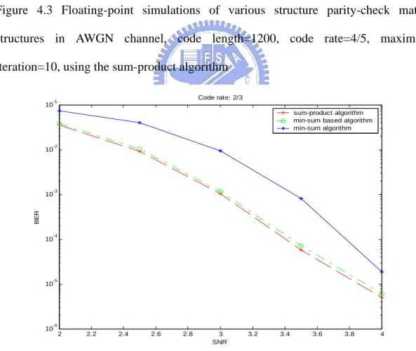
(10) structure, under the three decoding algorithm in AWGN channel, code length=720, code rate=2/3, maximum iteration=10.............................44 Figure 4.5. Floating-point simulations of the proposed parity-check matrix structure, under the three decoding algorithm in AWGN channel, code length=960, code rate=3/4, maximum iteration=10.............................45. Figure 4.6. Floating-point simulations of the proposed parity-check matrix structure, under the three decoding algorithm in AWGN channel, code length=1200, code rate=4/5, maximum iteration=10...........................45. Figure 4.7. Three different fixed-point simulation results of the proposed parity-check matrix structure, based on the sum-product decoding algorithm in AWGN channel, code length=720, code rate=2/3, maximum iteration=10.........................................................................47. Figure 4.8. Three different fixed-point simulation results of the proposed parity-check matrix structure, based on the min-sum based decoding algorithm in AWGN channel, code length=720, code rate=2/3, maximum iteration=10.........................................................................48. Figure 4.9. Three different fixed-point simulation results of the proposed parity-check matrix structure, based on the sum-product decoding algorithm in AWGN channel, code length=960, code rate=3/4, maximum iteration=10.........................................................................48. Figure 4.10. Three different fixed-point simulation results of the proposed parity-check matrix structure, based on the min-sum based decoding algorithm in AWGN channel, code length=960, code rate=3/4, maximum iteration=10.........................................................................49. Figure 4.11. Three different fixed-point simulation results of the proposed parity-check matrix structure, based on the sum-product decoding VIII.

(11) algorithm in AWGN channel, code length=1200, code rate=4/5, maximum iteration=10.........................................................................49 Figure 4.12. Three different fixed-point simulation results of the proposed parity-check matrix structure, based on the min-sum based decoding algorithm in AWGN channel, code length=1200, code rate=4/5, maximum iteration=10.........................................................................50. Figure 4.13. Two different fixed-point simulation results of the proposed parity-check matrix structure, based on the sum-product decoding algorithm in AWGN channel, code length=720, code rate=2/3, maximum iteration=10.........................................................................51. Figure 4.14. Two different fixed-point simulation results of the proposed parity-check matrix structure, based on the min-sum based decoding algorithm in AWGN channel, code length=720, code rate=2/3, maximum iteration=10.........................................................................51. Figure 4.15. Two different fixed-point simulation results of the proposed parity-check matrix structure, based on the sum-product decoding algorithm in AWGN channel, code length=960, code rate=3/4, maximum iteration=10.........................................................................52. Figure 4.16. Two different fixed-point simulation results of the proposed parity-check matrix structure, based on the min-sum based decoding algorithm in AWGN channel, code length=960, code rate=3/4, maximum iteration=10.........................................................................52. Figure 4.17. Two different fixed-point simulation results of the proposed parity-check matrix structure, based on the sum-product decoding algorithm in AWGN channel, code length=1200, code rate=4/5, maximum iteration=10.........................................................................53 IX.

(12) Figure 4.18. Two different fixed-point simulation results of the proposed parity-check matrix structure, based on the min-sum based decoding algorithm in AWGN channel, code length=1200, code rate=4/5, maximum iteration=10.........................................................................53. Figure 4.19. Floating-point vs. fixed-point simulation results of the proposed parity-check matrix structure for the sum-product and min-sum based algorithm in AWGN channel, code length=720, code rate=2/3, maximum iteration=10.........................................................................54. Figure 4.20. Floating-point vs. fixed-point simulation results of the proposed parity-check matrix structure for the sum-product and min-sum based algorithm in AWGN channel, code length=960, code rate=3/4, maximum iteration=10.........................................................................55. Figure 4.21. Floating-point vs. fixed-point simulation results of the proposed parity-check matrix structure for the sum-product and min-sum based algorithm in AWGN channel, code length=1200, code rate=4/5, maximum iteration=10.........................................................................55. Figure 5.1. Semi-parallel decoder for the proposed irregular LDPC code structure of rate 3/4, and code length 960...........................................................57. Figure 5.2. Illustration of overlapped decoding procedure ....................................59. Figure 5.3. ⎛ ⎛ x ⎞⎞ Function plot of φ ( x) = − ln⎜⎜ tanh⎜ ⎟ ⎟⎟ ..............................................60 ⎝ 2 ⎠⎠ ⎝. Figure 5.4. Architecture of check node function unit for the sum-product algorithm ..............................................................................................................61. Figure 5.5. Architecture of a 4-input variable node function unit for the sum-product algorithm.........................................................................61. Figure 5.6. Reformulated architecture of check node function unit for the. X.

(13) sum-product algorithm.........................................................................63 Figure 5.7. Reformulated architecture of a 4-input variable node function unit for the sum-product algorithm...................................................................63. Figure 5.8. Re-mapped architecture performing both check node update and variable node update operations for the sum-product algorithm .........65 −x. Figure 5.9. Function plot of g ( x) = ln(1 + e. Figure 5.10. Function plot of h( x) = ln(e x − 1) .......................................................67. Figure 5.11. Architecture of check node function unit for the min-sum based. ) ....................................................66. algorithm ..............................................................................................68 Figure 5.12. Architecture of a 4-input variable node function unit for the min-sum based algorithm....................................................................................68. XI.

(14) Chapter 1 Introduction. With the continuous growth of wireless communication technology, people have eventually become addicted to wireless products such as mobile phones and wireless LAN due to the convenience and enjoyment it has brought to our lives. However, the resources of the wireless frequency spectra are limited and valuable. The improvement of transmission efficiency for wireless communication has therefore become the focus of research in communication systems. The use of error correction codes is one of the main solutions to raising the transmission efficiency. Among various error correction codes, one called low-density parity-check code (LDPC) should be especially taken into account. LDPC codes were first presented by Gallager [1] in 1962 and have received great attention recently due to, its near Shannon limit coding gain when iterative decoded [2]. LDPC codes are currently widely considered a serious competitor to the turbo codes. The main advantages of LDPC codes over turbo codes are that LDPC decoders are known to require an order of magnitude less arithmetic computations, and the decoding algorithm for LDPC codes is parallelizable and can potentially be accomplished at significantly greater speeds. The disadvantage of the LDPC codes is the high complexity required in encoding. Recently, several efficient encoding approaches have been proposed [3,4,5]. In [5], it introduced an approach that used difference families to construct irregular quasi-cyclic codes free of 1.

(15) 4-cycles while reducing the encoding complexity to become linear to the code length. However, the performance was not as good as expected. The aim of this thesis is to construct a new structure of LDPC codes that improves the performance while using the concept of the difference families, and contact VLSI design of the corresponding decoder. This thesis is organized as follows. In chapter 2, basic concept of the LDPC codes including the code construction, encoding and decoding will be introduced. Chapter 3 will propose a new structure of LDPC codes by using difference families. In chapter 4, the simulation results for the LDPC codec will be discussed in chapter 2 and chapter 3 will be shown. Chapter 5 will discuss the VLSI implementation of the LDPC decoder. In the end of this thesis, brief conclusions will be presented in chapter 6.. 2.

(16) Chapter 2 Low-Density Parity-Check Code. In this chapter, an introduction to low-density parity-check code will be given, including the fundamental concepts of LDPC code, code construction, encoding and decoding mechanism.. 2.1 Fundamental Concept of LDPC Code. A binary LDPC code is a binary linear block code that can be defined by a sparse binary m × n parity-check matrix. A sparse matrix is a matrix where only a small fraction of its entries are ones. Non-binary LDPC codes over GF(q) are discussed in [6]. Hereafter, binary LDPC codes will be called LDPC codes for short. For any m × n parity-check matrix H, it defines a (n, j, k)-regular LDPC code if every column vector of H has the same weight j and every row vector of H has the same weight k. Here the weight of a vector is the number of ones in the vector. By counting the ones in H, it follows that n × j = m × k . Hence if m < n , then j < k . Suppose the parity-check matrix has full rank, the code rate of H is. r = (n − m) / n = (k − j ) / k = 1 − j / k . If not all the columns or all the rows of the parity-check matrix H have the same number of ones, an LDPC code is said to be irregular.. 3.

(17) As suggested by Tanner [7], an LDPC code can be represented as a bipartite graph. An LDPC code corresponds to a unique bipartite graph and a bipartite graph also corresponds to a unique LDPC code. In a bipartite graph, one type of nodes, called the variable nodes, correspond to the symbols in a codeword. The other type of nodes, called the check nodes, correspond to the set of parity check equations. If the parity-check matrix H were an m × n matrix, it would have m check nodes and n variable nodes. A variable node vi is connected to a check node cj by an edge, denoted as (vi, cj), if and only if the entry hi,j of H is one. A cycle in a graph of nodes and edges is defined as a sequence of connected edges which starts from a node and ends at the same node, and satisfies the condition that no node (except the initial and final node) appears more than once. The number of edges on a cycle is called the length of the cycle. The length of the shortest cycle in a graph is called the girth of the graph. Regular LDPC codes are those where all nodes of the same type have the same degree. The degree of a node is the number of edges connected to that node. For example, Figure2.1 shows a (8, 4, 2)-regular LDPC code and its corresponding. ⎡1 ⎢1 H =⎢ ⎢0 ⎢ ⎣0. 0 0. 1 0. 0 1. 1 0. 0 1. 1 0. 1 1. 1 0. 0 1. 0 1. 1 0. 1 0. c1. 0⎤ 1 ⎥⎥ 0⎥ ⎥ 1⎦ c3. c2. c4. check nodes. variable. nodes v1. v3. v2. v4. v5. v6. v7. v8. Figure 2.1 Example of a (8, 4, 2)-regular LDPC code and its corresponding Tanner graph.. There are 8 variable nodes (vi) and 4 check nodes (ci). 4.

(18) Tanner graph. In this example, all the variable nodes have a degree of 2 and all the check nodes have a degree of 4. The edges (c1, v3), (v3, c3), (c3, v7), and (v7, c1) depict a cycle in the Tanner graph. Since this turns out to be the shortest cycle, the girth of this graph is 4. Irregular LDPC codes were introduced in [8] and [9]. For such codes, the degrees of each set of nodes are chosen according to some distribution. A polynomial γ (x) of the form. γ ( x) = ∑ γ i x i −1. (2.1). i≥2. is a degree distribution if γ (x) has nonnegative coefficients and γ (1) = 1 .. Given a. degree distribution pair (λ , ρ ) to form a sequence of code ensembles C n (λ , ρ ) , where n is the length of the code and where dv. λ ( x) = ∑ λi x i −1 i=2. (2.2). dv. ρ ( x) = ∑ ρ i x. i −1. i=2. specify the variable and check node degree distributions. More precisely, λi and ρ i represent the fraction of edges emanating from variable and check nodes of degree i respectively; d v and d c are denoted as the maximum variable and check node degree. Assume that the code has n variable nodes. The number of variable nodes of degree i is then. n. λi / i λ /i =n 1 i ∑ λ j / j ∫ λ ( x)dx j ≥2. 0. dv d 1 v ⎛ 1 x i 1 dv λ ⎞ ⎜⎜ ∫ λ ( x)dx = ∫ ∑ λi x i −1dx = ∑ λi | = ∑ i ⎟⎟ 0 i 0 i =2 i ⎠ i =2 i =2 ⎝ 0. and so the total number of edges emanating from all variable nodes E is equal to. 5. (2.3).

(19) ⎛ ⎞ ⎜ ⎟ λi / i E = ∑⎜n 1 ⋅i⎟ = i≥2 ⎜ λ ( x)dx ⎟ ⎝ ∫0 ⎠. n 1. ∫. 0. λ ( x)dx. (2.4). Similarly, assuming that the code has m check nodes, E can also be expressed as. E=. m 1. ∫. 0. (2.5). ρ ( x)dx. Since the number of edges emanating from all variable nodes is equal to that emanating from all check nodes, we have E=. n 1. ∫. 0. λ ( x)dx. =. m 1. ∫. 0. ρ ( x)dx. (2.6). Hence 1. ∫ ρ ( x)dx m=n ∫ λ ( x)dx 0 1. (2.7). 0. Assuming that H has full rank, the rate of LDPC codes in the ensemble is ∆. r (λ , ρ ) =. n−m = 1− n. 1. ∫ λ ( x)dx ∫ ρ ( x)dx 0 1. (2.8). 0. Further more, the average degree j of a variable node and average degree k of a check node are. j=. E = n. 1. =. dv. ∑λ j =2. j. /j. 1 1. ∫ λ ( x)dx 0. (2.9). k=. E = m. 1. =. dc. ∑ρ j =2. j. /j. 6. 1 1. ∫ ρ ( x)dx 0.

(20) 2.2 Code Construction Gallager’s method [1]. Define an (n, j, k) parity-check matrix as a matrix of n columns that has j ones in each column, k ones in each row, and zeros elsewhere. In follows from this definition than an (n, j, k) parity-check matrix has nj / k rows and thus a rate r ≥ 1 − j / k . In order to construct an ensemble of (n, j, k) matrices, consider first the special (n, j, k) matrix in Figure 2.2, for which n, j and k will be 20, 3 and 4, respectively.. 1 1 1 1 0 0 0 0 0 0 0 0 0 0 0 0 0 0 0 0 0 0 0 0 1 1 1 1 0 0 0 0 0 0 0 0 0 0 0 0 0 0 0 0 0 0 0 0 1 1 1 1 0 0 0 0 0 0 0 0 0 0 0 0 0 0 0 0 0 0 0 0 1 1 1 1 0 0 0 0 0 0 0 0 0 0 0 0 0 0 0 0 0 0 0 0 1 1 1 1 1 0 0 0 1 0 0 0 1 0 0 0 1 0 0 0 0 0 0 0 0 1 0 0 0 1 0 0 0 1 0 0 0 0 0 0 1 0 0 0 0 0 1 0 0 0 1 0 0 0 0 0 0 1 0 0 0 1 0 0 0 0 0 1 0 0 0 0 0 0 1 0 0 0 1 0 0 0 1 0 0 0 0 0 0 0 0 1 0 0 0 1 0 0 0 1 0 0 0 1 1 0 0 0 0 1 0 0 0 0 0 1 0 0 0 0 0 1 0 0 0 1 0 0 0 0 1 0 0 0 1 0 0 0 0 1 0 0 0 0 0 0 1 0 0 0 0 1 0 0 0 0 1 0 0 0 0 0 1 0 0 0 0 1 0 0 0 0 1 0 0 0 0 1 0 0 1 0 0 0 0 0 0 0 1 0 0 0 0 1 0 0 0 0 1 0 0 0 0 1 Figure 2.2 Example of a low-density parity-check code matrix where (n, j, k) = (20, 3, 4) This matrix is divided into j sub-matrices, each containing a single 1 in each column. The first of these sub-matrices contains all its 1’s in descending order which is, the ith row contains 1’s in columns (i − 1)k + 1 to ik . The other sub-matrices are. 7.

(21) merely column permutations of the first. We define the ensemble of (n, j, k) codes as the ensemble resulting from random permutations of the columns of each of the bottom ( j − 1) sub-matrices of a matrix such as in Figure 2.2 with equal probability assigned to each permutation. This definition is somewhat arbitrary and is made for mathematical convenience. In fact such an ensemble does not include all (n, j, k) codes as just defined. Also, at least ( j − 1) rows in each matrix of the ensemble are linearly dependent. This simply means that the codes have a slightly higher information rate than the matrix indicates.. MacKay’s method [10] A computer-generated code was introduced by MacKay [10]. The parity-check matrix is randomly generated. First, the parameters n, m, j, and k are chosen to conform an (n, m, j, k)-regular LDPC code where n, j and k are the same as in Gallager’s code and m is the number of the parity-check equations in H. Then, 1’s are randomly generated into j different positions of the first column. The second column is generated in the same way, but checks are made to insure that no two columns have a 1 in the same position more than twice. This constraint is to avoid a 4-cycle to appear in the Tanner graph, which will cause the performance to drop by about 0.5dB. An avoidance of 4-cycles in a parity-check matrix is therefore required. The next few columns are generated sequentially and checks for 4-cycles must be performed on each generation. In this procedure, the number of 1’s in each row must be recorded, and if any row already has k 1’s, the next column generating will not select that row.. 8.

(22) Construction by Quasi-Cyclic Code [5]. A code is quasi-cyclic if, for any cyclic shift of a codeword by l places, the resulting word is also a codeword. A cyclic code is a quasi-cyclic code with l = 1 .. Consider the binary quasi-cyclic codes described by a parity-check matrix H = [ A1 , A2 ,... Al ] where A1 , A2 ,... Al are binary v × v circulant matrices. The algebra of. (2.10). (v × v ). binary circulant matrices is isomorphic to the algebra of polynomials modulo x v − 1 over GF(2). A circulant matrix A is completely characterized by the polynomial. a( x) = a 0 + a1 x + a 2 x 2 + .... + a v −1 x v −1. (2.11). where the coefficients are from the first row of A , and a code C with parity-check matrix of the form (2.10) can be completely characterized by the polynomials a1 ( x), a 2 ( x),..., al ( x) .. Figure2.3(a) shows an example of a rate-1/2 quasi-cyclic code. where a1 ( x) = 1 + x and a 2 ( x) = 1 + x 2 + x 4 . Figure2.3(b) shows the corresponding Tanner graph representation.. For this example we can see the edges (c1, v6), (v6, c4),. (c4, v8), (v8, c1) depict a 4-cycle in this graph which is to be avoided for performance consideration. The method for avoiding 4-cycle condition will be discussed in the next chapter.. ⎡1 ⎢ ⎢0 H = ⎢0 ⎢ ⎢0 ⎢1 ⎣. 1 0 0 0 1 0 1 0 1⎤ ⎥ 1 1 0 0 1 1 0 1 0⎥ 0 1 1 0 0 1 1 0 1⎥ ⎥ 0 0 1 1 1 0 1 1 0⎥ 0 0 0 1 0 1 0 1 1⎥⎦. (a) A parity-check matrix with two circulant matrices. 9.

(23) c1. c3. c2. c5. c4. check nodes. variable nodes v1. v2. v3. v4. v5. v6. v7. v8. v9. v10. (b) Tanner graph representation Figure2.3 Example of a rate-1/2 quasi-cyclic code from two circulant matrices, where a1 ( x) = 1 + x and a 2 ( x) = 1 + x 2 + x 4. 2.3 Encoding. Since LDPC code is a linear block code, it can be encoded by the conventional method. However, using conventional method will introduce an encoding complexity proportional to the quadratic of the code length. The high encoding cost of LDPC codes becomes a major drawback when compared to the turbo codes which has a linear encoding complexity with time. In this section, we will introduce some improved methods.. Conventional method. Let u = [u 0 , u1 , u 2 ,..., u k −1 ] be a row vector of message bits with length k and c = [c 0 , c1 , c 2 ,..., c n −1 ] be a codeword with length n. Let G with dimension k × n be the generating matrix of this code. It can be derived that c = uG .. (2.12). If H is the parity-check matrix of this code with dimension r × n where r = n − k . Then 10.

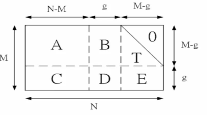
(24) Hc T = 0T ⇒ cH T = 0 ⇒ uGH T = 0. (2.13). ⇒ GH = 0 T. Suppose a sparse parity-check matrix H with full rank is constructed. Gaussian elimination and column reordering can be used to derive an equivalent parity-check matrix in the systematic form H systematic = [ P I r ] . Thus equation (2.13) can be solved to get the generating matrix in systematic form as. G systematic = [ I k P T ] .. (2.14). Finally, the generating matrix G can be obtained by doing the reverse column reordering to the G systematic .. Forcing H to have lower triangular form [4]. In [4] it was suggested to force the parity-check matrix to be in the lower triangular form. Under this restriction, it guarantees a linear time encoding complexity, but, in general, it also results in some loss of performance.. Richardson’s method [3]. Figure 2.4 shows how to bring the parity-check matrix into an approximate lower triangular form using row and column permutations. Note that since this. 11.

(25) Figure 2.4 The parity-check matrix in an approximate lower triangular form transformation was accomplished solely by permutations, the matrix is still sparse. More precisely, assume that the matrix is written in the form ⎛A B T⎞ ⎟⎟ H = ⎜⎜ C D E ⎝ ⎠. (2.15). where A is (m − g ) × (n − m) , B is (m − g ) × g , T is (m − g ) × (m − g ) , C is. g × (n − m) , D is g × g , and E is g × (m − g ) . Further, all these matrices are sparse and T is lower triangular with ones along the diagonal. Multiplying this matrix from the left by ⎛ I ⎜⎜ −1 ⎝ − ET. 0⎞ ⎟ I ⎟⎠. (2.16). can result in A ⎛ ⎜⎜ −1 ⎝ − ET A + C. T⎞ ⎟. − ET B + D 0 ⎟⎠ B. −1. (2.17). Let x = ( s, p1 , p 2 ) denote the codeword of this parity-check matrix where s is the message bits with length (m − n) , p1 and p 2 combin ed are the parity bits, p1 has length g , and p 2 has length (m − g ) . The constrained equation Hx T = 0 T splits naturally into two equations, namely As T + Bp1T + Tp 2T = 0. (2.18). and. (− ET. −1. ). (. ). A + C s T + − ET −1 B + D p1T = 0 .. (2.19). Define γ = − ET −1 B + D and assume for the moment that γ is nonsingular. Then 12.

(26) from equation (2.19) we conclude that. (. ). p1T = −γ −1 − ET −1 A + C s T .. (. (2.20). ). Hence, once the g × (n − m) matrix − γ −1 − ET −1 A + C s T has been pre-computed, the determination of. p1 can be accomplished with a time complexity of. Ο( g × (n − m)) simply by performing a multiplication with this (generically dense) matrix. This complexity can be further reduced as shown in Table 2.1. Rather than. (. ). pre-computing − γ −1 − ET −1 A + C s T and then multiplying with s T , p1 can be determined by breaking the computation into several smaller steps, each of which is computationally efficient. To this end, we first determine As T , which has complexity of Ο(n) , since A is sparse. Next, we multiply the result by T −1 . Since T −1 [ As T ] = y T. is equivalent to the system [ As T ] = Ty T , this can also be. accomplished in Ο(n) time with by back-substitution, because T. is lower. triangular and sparse. The remaining steps are fairly straightforward. It follows that the overall complexity of determining p1 is Ο(n + g 2 ). In a similar manner, noting from equation (2.18) that. p 2T = −T −1 ( As T + Bp1T ) , we can accomplish the. determination of p 2 in time complexity of Ο(n) as shown step by step in Table 2.2. A summary of this efficient encoding procedure is given in Table 2.3. It entails two steps, the preprocessing step and the actual encoding step. In the preprocessing step, we first perform row and column permutations to bring the parity-check matrix into the approximate lower triangular form with as small a gap g as possible. In actual encoding then entails the steps listed in Table 2.1 and 2.2. The overall encoding complexity is Ο(n + g 2 ) , where g is the gap of the approximate triangulation.. 13.

(27) (. ). Table 2.1 Efficient computation step of p1T = −γ −1 − ET −1 A + C s T Operation. Comment. Complexity. As T. Multiplication by sparse matrix. Ο(n ). T −1 [ As T ]. T −1 [ As T ] = y T ⇔ [ As T ] = Ty T. Ο(n ). − E[T −1 As T ]. Multiplication by sparse matrix. Ο(n ). Cs T. Multiplication by sparse matrix. Ο(n ). [− ET −1 As T ] + [Cs T ]. Addition. Ο(n ). − γ −1[− ET −1 As T + Cs T ]. Multiplication by dense g × g matrix. Ο g2. ( ). Table 2.2 Efficient computation step of p 2T = −T −1 ( As T + Bp1T ) Operation. Comment. Complexity. As T. Multiplication by sparse matrix. Ο(n ). Bp1T. Multiplication by sparse matrix. Ο(n ). [ As T ] + [ Bp1T ]. Addition. Ο(n ). − T −1 [ As T + Bp1T ]. − T −1 [ As T + Bp1T ] = y T ⇔ −[ As T + Bp1T ] = Ty T. Ο(n ). Table 2.3 Summary of Richardson’s encoding procedure It entails two steps: A processing step and the actual encoding step Preprocessing: Input: Non-singular parity-check matrix H. Output: An equivalent ⎛A B T⎞ ⎟⎟ parity-check matrix of the form ⎜⎜ ⎝C D E ⎠. such that − ET −1 B + D. is. non-singular. 1. [Triangulation] Perform row and column permutations to bring the parity-check matrix H into the approximate lower triangular form ⎛A B T⎞ ⎟⎟ H = ⎜⎜ ⎝C D E ⎠ with as small a gap g as possible. 14.

(28) 2. [Check] Check that − ET −1 B + D is non-singular, performing further column permutations if necessary to ensure this property. ⎛ I ⎜⎜ −1 ⎝ ET. 0 ⎞⎛ A B T ⎞ ⎛ A ⎟⎟⎜⎜ ⎟⎟ = ⎜⎜ −1 I ⎠⎝ C D E ⎠ ⎝ − ET A + C. T⎞ ⎟ − ET B + D 0 ⎟⎠ ⎛A B T⎞ ⎟⎟ such that Encoding: Input: Parity-check matrix of the form ⎜⎜ ⎝C D E ⎠ B. −1. − ET −1 B + D is non-singular and a vector s denote the message bits has length. (m − n) . Output: The vector x = ( s, p1 , p 2 ) where p1 has length g and p 2 has length (m − g ) , such that Hx T = 0 T . 1. Determine p1 as shown in Table 2.1. 2. Determine p 2 as shown in Table 2.2.. Quasi-cyclic code [5]. As a review of quasi-cyclic code in section 2.2, the quasi-cyclic code can be described by a parity-check matrix H = [ A1 , A2 ,... Al ] and each of a circulant matrix. A j is completely characterized by the polynomial a ( x) = a 0 + a1 x + .... + a v −1 x v −1 with coefficients from its first row. A code C with parity-check matrix H can be completely characterized by the polynomials a1 ( x), a 2 ( x),..., al ( x) . As for the encoding, if one of the circulant matrices is invertible (say Al ) the generator matrix for the code can be constructed in the following systematic form ⎡ ⎢ G = ⎢ I v ( l −1) ⎢ ⎢ ⎣⎢. ( A l− 1 A 1 ) T ⎤ ⎥ ( A l− 1 A 2 ) T ⎥ ⎥ ... −1 T ⎥ ( A l A l − 1 ) ⎦⎥. (2.21). resulting in a quasi-cyclic code of length vl and dimension v(l − 1) . Encoding can be achieved with linear complexity using a v(l − 1) -stage shift register. Regarding the. 15.

(29) algebraic computation, the polynomial transpose is defined as n −1. a ( x ) T = ∑ a i x n −i , x n = 1 .. (2.22). i =0. For a binary [n, k] code, length n = vl and dimension k = v(l − 1) , the k-bit message. [i0 , i1 ,..., ik −1 ]. is described by the polynomial i ( x) = i0 + i1 x + ... + ik −1 x k −1 and the. codeword for this message is c( x) = [i ( x), x k p ( x)] , where p(x) is given by l −1. p ( x) = ∑ i j ( x) ∗ (al−1 ( x) ∗ a j ( x)) T ,. (2.23). j =1. i j (x) is the polynomial representation of the information bits iv ( j −1) to ivj −1 , where i j ( x) = iv ( j −1) + iv ( j −1) +1 x + ... + ivj −1 x v −1. (2.24). and polynomial multiplication (∗) is mod x v − 1 . As an example, consider a rate-1/2 quasi-cyclic code with v = 5 , l = 2 , first circulant is described by a1 ( x) = 1 + x and the second circulant is described by a 2 ( x) = 1 + x 2 + x 4 , which is invertible and. a 2− 1 ( x ) = x. + x2 + x4 .. (2.25). The generator matrix contains a 5 × 5 identity matrix and the 5 × 5 matrix described by the polynomial (a 2−1 ( x) ∗ a1 ( x)) T = (1 + x 2 ) T = 1 + x 3 .. (2.26). Figure 2.5 shows the example parity-check matrix and the corresponding generator matrix.. 16.

(30) ⎡1 ⎢ ⎢0 H = ⎢0 ⎢ ⎢0 ⎢1 ⎣. 1 0 0 0 1 0 1 0 1⎤ ⎥ 1 1 0 0 1 1 0 1 0⎥ 0 1 1 0 0 1 1 0 1⎥ ⎥ 0 0 1 1 1 0 1 1 0⎥ 0 0 0 1 0 1 0 1 1⎥⎦. (a) A parity-check matrix with two circulants ⎡1 ⎢ ⎢0 G = ⎢0 ⎢ ⎢0 ⎢0 ⎣. 0 0 0 0 1 0 0 1 0⎤ ⎥ 1 0 0 0 0 1 0 0 1⎥ 0 1 0 0 1 0 1 0 0⎥ ⎥ 0 0 1 0 0 1 0 1 0⎥ 0 0 0 1 0 0 1 0 1⎥⎦. (b)The corresponding generator matrix in systematic form Figure 2.5 Example of a rate-1/2 quasi-cyclic code. (a) Parity-check matrix with two circulants, where a1 ( x) = 1 + x and a 2 ( x) = 1 + x 2 + x 4 . (b) Corresponding generator matrix in systematic form.. 2.4 Decoding [11]. There are several decoding algorithm for LDPC codes. All of them are iterative decoding. Messages between variable nodes and check nodes are exchanged back and forth. The decoder expects that error will be corrected progressively by using this iterative message-passing algorithm. At present, there are three types of iterative decoding algorithms applied to LDPC codes in general.. Sum-product algorithms, also known as message passing algorithm. Min-sum based algorithms. Min-sum algorithms.. 17.

(31) 2.4.1 Decoding Procedure in One Iteration Now we make a description of the message passing algorithm in one iteration. Here is a simple example of irregular LDPC code. The parity check matrix is shown below.. ⎡1 H =⎢ ⎣1. 1 0. x1. 0⎤ 1 ⎥⎦. 0 1. x2. S1 S2. x4. x3. v v If the received codeword sequence is x , then we can use H x T = 0 T to try whether the received codeword sequence is a codeword, i.e.,. ⎡ x1 ⎤ ⎢ ⎥ ⎡1 1 0 0⎤ ⎢ x 2 ⎥ ⎡0⎤ T T =⎢ ⎥ Hx = O ⇒ ⎢ ⎥ ⎣1 0 1 1 ⎦ ⎢ x 3 ⎥ ⎣0⎦ ⎢ ⎥ ⎣x4 ⎦ ⇒. (2.27). Equation S1 : x1 ⊕ x2 = 0 Equation S 2 : x1 ⊕ x3 ⊕ x4 = 0. where “ ⊕ ” denotes the modulo-2 addition. The message passing algorithm uses Tanner graph for decoding procedure, which is shown below. S1. x1. x2. check node. S2. x3. x4. variable. node. For x1 estimation: Step1: Suppose. p0. and. p1 are the priori-probability of. x2 ,. where. p 0 + p1 = 1 , we can use Equation S1 ( x1 ⊕ x 2 = 0) to estimate the post-probability of x1 as follows:. 18.

(32) S1. x1. P ( x1 = 0) = P ( x 2 = 0) = p 0 P ( x1 = 1) = P ( x 2 = 1) = p1 .. x2. (2.28). ( p 0 , p1 ). In the same way, suppose q 0 and q1 are the priori-probability of x3 , where q 0 + q1 = 1 and r0 and r1 are the priori-probability of x 4 where r0 + r1 = 1 , we can use Equation S 2 that ( x1 ⊕ x3 ⊕ x 4 = 0) to estimate the post-probability of x1 , using the following equation: P ( x1 = 0) = P ( x 3 ⊕ x 4 = 0) = P ( x 3 = 0) P ( x 4 = 0) + P ( x 3 = 1) P ( x 4 = 1) = q 0 r0 + q1 r1 (2.29) P ( x1 = 1) = P ( x 3 ⊕ x 4 = 1) = P ( x 3 = 1) P ( x 4 = 0) + P ( x 3 = 0) P ( x 4 = 1) = q1 r0 + q 0 r1 S2. x1 Step2: Based on Equation S1. x3 x4 (q 0 , q1 ) (r0 , r1 ) and Equation S 2 , we can estimate the final. post-probability of x1 , by using:. P ( x1 = 0) ∝ P ( S1 = 0 and x1 = 0) P ( S 2 = 0 and x1 = 0) = p 0' q 0' P ( x1 = 1) ∝ P ( S1 = 0 and x1 = 1) P ( S 2 = 0 and x1 = 1) = p1' q1'. S1 ' 0. (2.30). S2. ' 1. (p , p ). ( q 0' , q1' ). x1 where p 0' = p 0 , p1' = p1 , q 0' = q 0 r0 + q1 r1 and q1' = q1 r0 + q 0 r1 . It can be summed up that if a check node S i is connected by three variable nodes x i , x j and x k , and if the priori-probability of the variable nodes x i and x j are (q 0 , q1 ) and 19.

(33) (r0 , r1 ) , respectively, we can use the check Equation S i to estimate the post-probability of x k in step1 which is CHK (q 0 , q1 , r0 , r1 ) = (q 0 r0 + q1 r1 , q1 r0 + q 0 r1 ) .. (2.31). Similarly, if a variable node x i is connected by two check nodes that are S i and. S j , and if the message of the S i and S j are collected from step1 are ( p 0' , p1' ) and (q 0' , q1' ) , respectively, we can estimate the final post-probability of x i as ⎛ ⎞ p' q' p' q' VAR( p0' , p1' , q0' , q1' ) = ⎜⎜ ' ' 0 0 ' ' , ' ' 1 1 ' ' ⎟⎟ . ⎝ p0 q0 + p1 q1 p0 q0 + p1 q1 ⎠. (2.32). Since the summation of the priori-probability on any variable node x k is one, in other words p 0 + p1 = 1 , we can transform the priori-probability to a single-value function. Let L( p o , p1 ) = ln. po = ln λ , then equations (2.31) and (2.32) can be p1. rewritten as. CHK ( L1 , L2 ) = CHK ( L1 ⊕ L2 ) = ln −. 1 + λ1λ 2 λ1 + λ 2. L1 + L2 2. L1 + L2 2. +e 1+ e e e = ln L1 − L2 L1 L2 L −L − 1 2 e +e e 2 +e 2 L + L2 L − L2 = ln(cosh( 1 )) − ln(cosh( 1 )) 2 2 L L = 2 tanh −1 (tanh( 1 ) × tanh( 2 )) 2 2 = ln. L1. L2. VAR ( L1 , L2 ) = ln(λ1λ 2 ) = ln λ1 + ln λ 2 = L1 + L2 .. (2.33). (2.34). Equations (2.33) and (2.34) are computation in Log-Likelihood Ratio (LLR) form. This transform can reduce the number of parameters, and equation (2.34) VAR ( L1 , L2 ) only needs an addition operation rather than multiplication.. Furthermore, equation (2.33) can be further reformulated to different manners.. 20.

(34) There are. L1 L ) × tanh( 2 )) 2 2 = sign( L1 ) sign( L2 )φ (φ ( L1 ) + φ ( L2 )). CHK ( L1 ⊕ L2 ) = 2 tanh −1 (tanh(. (2.35). where ⎛ x ⎞⎞. ⎛. ⎛ ex +1⎞. φ ( x) = − ln⎜⎜ tanh⎜ ⎟ ⎟⎟ = ln⎜⎜ x ⎟⎟ and φ (φ ( x)) = x , ⎝ 2 ⎠⎠ ⎝ ⎝ e −1⎠. (2.36). and. L1 + L2 L − L2 )) − ln(cosh( 1 )) 2 2 − L +L L1 + L2 L1 − L2 1+ e 1 2 = − + ln − L −L 2 2 1+ e 1 2. CHK ( L1 ⊕ L2 ) = ln(cosh(. = sign(L1 ) × sign(L 2 ) × min( L1 , L2 ) + ln. 1+ e. − L1 + L2. 1+ e. − L1 − L2. ≈ sign( L1 ) × sign( L2 ) × min( L1 , L2 ) .. (2.37) (2.38). When the check node computation is in the form of equation (2.35), we call it the sum-product algorithm. Similarly, when the check node computation is in the form of equation (2.37), we call it the min-sum based algorithm, and the fourth term ln. 1+ e. − L1 + L2. 1+ e. − L1 − L2. in equation (2.37) is called the correction factor. Last of all, when the. check node computation is the form of equation (2.38), or in other words an approximate form, we call it the min-sum algorithm. The above discussion of check node computation is only about a check node connected by two or three variable nodes. Now, we will discuss the case when the number of variable nodes are more than three, and then discuss the general form. Consider a check node S 1 connected by four variable nodes x1 , x 2 , x 3 and x 4 . The priori-probability of variable nodes x1 , x 2 and x 3 are ( p 0 , p1 ) , (q 0 , q1 ). and. (r0 , r1 ) .. We. can. use. the. check. Equation. x1 ⊕ x 2 ⊕ x 3 ⊕ x 4 = 0 to estimate the post-probability of x 4 , namely, 21. S1 ,. that. is,.

(35) P ( x 4 = 0) = P ( x1 ⊕ x 2 ⊕ x 3 = 0) = P ( x1 = 0) P ( x 2 = 0) P ( x 3 = 0) + P ( x1 = 1) P ( x 2 = 1) P ( x 3 = 0) + P ( x1 = 0) P ( x 2 = 1) P ( x 3 = 1) + P ( x1 = 1) P ( x 2 = 0) P ( x3 = 1) = p 0 q 0 r0 + p1 q1 r0 + p 0 q1 r1 + p1 q 0 r1 P ( x 4 = 1) = P ( x1 ⊕ x 2 ⊕ x 3 = 1) = P ( x1 = 1) P ( x 2 = 1) P ( x 3 = 1) + P ( x1 = 1) P ( x 2 = 0) P ( x 3 = 0) + P ( x1 = 0) P ( x 2 = 1) P ( x 3 = 0) + P ( x1 = 0) P ( x 2 = 0) P ( x3 = 1) = p1 q1 r1 + p1 q 0 r0 + p 0 q1 r0 + p 0 q 0 r1 (2.39) S1. x1 ( p 0 , p1 ). x3 x2 x4 ( q 0 , q 1 ) ( r0 , r1 ). Then, one can transform equation (2.39) to a LLR form, and obtain CHK ( L1 ⊕ L2 ⊕ L3 ) = ln. = ln. λ λ λ + λ1 + λ 2 + λ3 p 0 q 0 r0 + p1 q1 r0 + p 0 q1 r1 + p1 q 0 r1 = ln 1 2 3 p1 q1 r1 + p1 q 0 r0 + p 0 q1 r0 + p 0 q 0 r1 1 + λ1λ 2 + λ 2 λ3 + λ3 λ1 e e e +e +e +e = ln 1 + e L1 e L2 + e L2 e Le + e Le e L1 L1. L2. Le. L1. L3. L2. x + L3. −. ⎡1 + e L1 e L2 1 + ⎢ L1 L2 ⎣e +e. ⎤ L3 ⎥+e ⎦. 1 + e L1 e L2 + e L3 L1 L2 e +e. x + L3. 1 + e x e L3 e 2 +e 2 ln = = ln x x − L3 x − L3 − e + e L3 2 e +e 2. ⎛ ⎛ ⎛ x + L3 ⎞ ⎞ ⎛ x − L3 ⎞ ⎞ = ln⎜⎜ cosh ⎜ ⎟ ⎟⎟ − ln⎜⎜ cosh ⎜ ⎟ ⎟⎟ 2 2 ⎝ ⎝ ⎠ ⎠⎠ ⎠ ⎝ ⎝ ⎛ ⎛ L ⎞⎞ ⎛ x⎞ = 2 tanh −1 ⎜⎜ tanh ⎜ ⎟ tanh ⎜ 3 ⎟ ⎟⎟ ⎝2⎠ ⎝ 2 ⎠⎠ ⎝. (2.40). 1 + e L1 e L2 1 + e L1 e L2 x ⇒e = L . From equation (2.33), it can be seen that where x = ln L e 1 + e L2 e 1 + e L2 x = CHK ( L1 ⊕ L2 ) . Equation (2.40) can be computed in a recursive manner such that. CHK ( L1 ⊕ L2 ⊕ L3 ) = CHK (CHK ( L1 ⊕ L2 ) ⊕ L3 ) . The general form for check node. 22.

(36) computation can be derived as CHK ( L1 ⊕ L2 ⊕ ... ⊕ Ll ) = CHK (CHK (...CHK (CHK ( L1 ⊕ L2 ) ⊕ L3 )...) ⊕ Ll ) . (2.41) Similarly, consider that a variable node x1 connected by three check nodes S1 , S 2 and S 3 , and the message collected by S1 , S 2 and S 3 are ( p 0 , p1 ) , (q 0 , q1 ) and (r0 , r1 ) , respectively. The final post-probabilities of the variable node x1 are P ( x1 = 0) = P( S1 = 0 and x1 = 0) P ( S 2 = 0 and x1 = 0) P ( S 3 = 0 and x1 = 0) = p 0 q 0 r0 P ( x1 = 1) = P ( S1 = 0 and x1 = 1) P ( S 2 = 0 and x1 = 1) P ( S 3 = 0 and x1 = 1) = p1 q1 r1 .. S1. S 2 ( q 0 , q1 ). ( p 0 , p1 ). (2.42). S3 ( r0 , r1 ). x1 Then, one can transform equation (2.38) into a LLR form, and obtain VAR ( L1 , L2 , L3 ) = ln(λ1λ 2 λ3 ) = ln λ1 + ln λ 2 + ln λ3 = L1 + L2 + L3 .. (2.43). So equation (2.43) can also be computed in a recursive manner such that VAR ( L1 , L2 , L3 ) = VAR (VAR ( L1 , L2 ), L3 ) , and the general form to the variable node computation can be derived as VAR ( L1 , L2 ,..., Ll ) = VAR (VAR...(VAR (VAR ( L1 , L2 ), L3 )...), Ll ) .. (2.44). 2.4.2 Iterative Decoding Procedure [12]. The discussion in section 2.4.1 is about the decoding procedure in one iteration. Now, we consider the actual decoding procedure. It means that there will involve many iterations for a decoding process. First, let us describe some notations for the iterative decoding procedure in Figure 2.6. M (l ) denotes the set of check nodes that are connected to the variable node l , i.e., positions of “1”s in the l th column of the 23.

(37) parity-check matrix. L(m) denotes the set of variable nodes that participate in the. m th parity-check equation, i.e., the positions of “1”s in the m th row of the parity-check matrix. L(m) \ l represents the set L(m) excluding the l th variable node and M (l ) \ m represents the set M (l ) excluding the m th check node. ql ,m denotes the. Variable node index l. Check node index m. ⎡ ⎢ ⎢ ⎢ ⎢ ⎢ ⎢ ⎢ ⎢ ⎢ ⎢ ⎢ ⎢ ⎢ ⎣. 1. M (1) \1. L(3) \1. L(3). M (1). 0. 0. 0. 0. 0 1. 0. 0. 0 1. 1 1. 0 0 1 1 1 1 0 0. 0. 0. 0. 0 1. 0 1. 0 1. ⎥. 0⎥ ⎥. 0 0 0⎥⎥ ⎥ 0 0 0⎥⎥. 0 1. 0 1. 1. 1⎤⎥. 0 1⎥⎥. 0 1. ⎥. 0⎥⎦. Figure 2.6 Notations for iterative decoding procedure probability message that variable node l sends to check node m . rm ,l denotes the probability message that the m th check node gathers for the l th variable node. The probability message of ql ,m and rm ,l are computation in LLR domain. The iterative decoding procedure is shown below.. 1. Initialization Let Ll = ln. P ( y l x l = 0) P ( y l xl = 1). =. 2. σ2. yl. (2.45). be the log likelihood ratio of a variable node, where P (a b) specifies that given b is transmitted, the probability that the receiver received a, where σ 2 is the noise variance. For every position (m, l ) such that H m ,l = 1 , q m,l is initialized as. q m,l = Ll . 24. (2.46).

(38) 2. Message passing Step1 (message passing from check nodes to variable nodes): Each check node m gathers all the incoming message q m,l ’s, and update the message on the variable. node l based on the messages from all other variable nodes connected to the check node m . rm ,l = CHK (∑ ⊕q m ,l ' ) .. (2.47). l ' ∈L ( m ) \ l. Step2 (message passing from variable nodes to check nodes): Each variable node l passes its probability message to all the check nodes that are connected to it.. q m ,l = VAR( VAR (rm ',l ), Ll ) = Ll + m '∈M ( l ) \ m. ∑r. m ',l m '∈M ( l ) \ m. .. (2.48). Step3 (decoding): For each variable node l , messages from all the check nodes that are connected to the variable node l are summed up.. ql = VAR( VAR (rm ,l ), Ll ) = Ll + m∈M ( l ). ∑r. m ,l m∈M ( l ). .. (2.49). Hard decision is made on q l , and the resulting decoded input vector xˆ is checked against the parity-check matrix H . If Hxˆ T = 0 , the decoder stops and output xˆ . Otherwise it repeats steps 1-3 until it reaches the specified maximum iteration loops.. 2.4.3 Efficient Check Node Computation. According to equation (2.41), the check node update computation can be implemented in a serial configuration. Consider a particular check node m with l connections from variable nodes. The incoming messages are then q m ,1 , q m , 2 ,..., q m ,l . The goal is to compute the outgoing messages rm ,1 , rm , 2 ,..., rm ,l . Let us define two sets of. auxiliary. binary. random. variables. 25. f1 = q m,1 ,. f 2 = f1 ⊕ q m, 2 ,.

(39) f 3 = f 2 ⊕ q m ,3 , …. ,. f l = f l −1 ⊕ q m,l , and. bl = q m ,l ,. bl −1 = bl ⊕ q m ,l −1 ,…,. b1 = b2 ⊕ q m,1 . We can obtain CHK ( f1 ) , CHK ( f 2 ) , …, CHK ( f l ) and CHK (b1 ) , CHK (b2 ) , …, CHK (bl ) in a recursive manner based on the knowledge of. q m ,1 , q m , 2 ,..., q m ,l . Using the parity-check node constraint (q m,1 ⊕ q m , 2 ⊕ ... ⊕ q m ,l ) = 0 , the outgoing message from check node m can be simply expressed as rm ,i = CHK ( f i −1 ⊕ bi +1 ), i = 2,3,..., l − 1, rm ,1 = CHK (b2 ),. (2.50). rm ,l = CHK ( f l −1 ). The total computational load consists of the forward recursive computation of CHK ( f i ) , the backward recursive computation of CHK (bi ) , and the final pair-wise part in equation (2.50), which amounts to 3(l − 1) core operation of the type. CHK (a ⊕ b) per check node. Clearly, the above procedure is exactly the forward-backward algorithm, as shown in Figure 2.7. The serial nature of computations makes a latency of O(l ) units of time in computing a check node update.. Figure 2.7 Serial configuration for computing check node update An efficient implementation for computing check node update is introduced by 26.

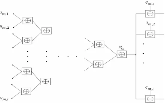
(40) [13]. A simple parallel configuration that enables fast check node update is described l. here. First, an auxiliary binary random variable S m = ∑ ⊕ q m ,i is defined. Then, S m i =1. can be computed using the parallel configuration shown in Figure 2.8. The computation at each check node in the parallel configuration is CHK (a ⊕ b) . The latency in computing the S m is of order O(log l ) , resulting in a speed-up factor of O[d c log(l )] compared to the serial configuration. Having obtained S m , the. i = 1,2,..., l , can be computed in an efficient way. Consider. outgoing message r. m. ,. i. ,. l. CHK ( S m ) = CHK ( ∑ ⊕ q m ,i ) = CHK ( q m ,i ⊕ i =1. = ln. 1+ e. l. ∑. CHK(. j = 1 ,j ≠ i. l. CHK(. e. ∑. j = 1 ,j ≠ i. l. ∑⊕q. j =1, j ≠ i. m, j. ). ⊕ q m,j ) + q m,l. .. ⊕ q m,j ). +e. (2.51). q m,l. l. Since the term CHK (. ∑⊕ q. j =1, j ≠ i. m, j. ) in equation (2.51) is exactly equivalent to the. outgoing message rm ,i from check node m to all the variable nodes i, where. i ∈ (1,2,..., l ) , equation (2.51) becomes 1 + e m ,i r. CHK ( S m ) = ln. + qm , i. e m ,i + e r. qm ,i. .. (2.52). Then, rm ,i can be obtained by reformulating equation (2.52) as. 1 + e m ,i r. e. CHK ( S m ). =. e. rm , i. + qm ,i. +e. qm , i. ⇒ e m ,i r. + CHK ( S m ). ⇒ e m,i (e r. qm , i. ⇒ e m,i =. e. ⇒ e m,i =. e. r. r. e e. +e. qm , i + CHK ( S m ). − e CHK ( S m ) ) = e. q m , i + CHK ( S m ) qm , i. −e. −1. CHK ( S m ). q m , i + CHK ( S m ). −1. q m , i −CHK ( S m ). −1. ⇒ rm ,i = ln. e e. =. + qm , i. q m , i + CHK ( S m ). −1. r. e (e. q m , i + CHK ( S m ). qm , i −CHK ( S m ). −1. − 1) × e CHK ( S m ). × e −CHK ( S m ). qm , i + CHK ( S m ). −1. qm , i −CHK ( S m ). −1. 27. = 1 + e m ,i. − CHK ( S M ) .. (2.53).

(41) Lastly, let’s define. rm ,i = CHK ( S m. q m,i ), where i = 1,2,..., l .. (2.54). It can be seen that for each i ∈ {1,2,..., l} , the message rm ,i can be computed simultaneously by a parallel implementation of the new core computation CHK ( S m. q m,i ) as shown in Figure 2.8. Clearly, only l − 1 core computation of. type CHK (a ⊕ b) and l core computation of type CHK (a. b) are necessary for. a particular check node update in this parallel configuration.. Figure 2.8 Parallel configuration for computing check node update In the end of this section, we synthesize the contents discussed in sections 2.4.1, 2.4.2 and 2.4.3, and give a summary to the sum-product algorithm, min-sum based algorithm and min-sum algorithm in Table 2.4, Table 2.5 and Table 2.6, respectively.. 28.

(42) Table 2.4 Summary of the sum-product algorithm 1. Initialization: For 1 ≤ l ≤ n L l = ln. P ( yl xl = 0) P ( y l x l = 1). =. 2. σ. For every l , m such that H. 2. y l , where σ. m ,l. 2. is the noise variance. =1. q m ,l = L l. 2. Message passing: Step1: Message passing from check nodes to variable nodes. For each l, m , compute. rm ,l = CHK (q m ,l ' ) = CHK (∑ ⊕q m ,l ' ) l ' ∈L ( m ) \ l. = sign(q m ,l ). l ' ∈L ( m ) \ l. ∏. l ′∈L ( m ). sign(q m,l ′ ) × φ (φ (. ∑q. l ′∈L ( m ). m ,l ′. ) − φ ( q m ,l ). ⎛ ex +1⎞ ⎛ ⎛ x ⎞⎞ ⎟⎟ and φ (φ ( x)) = x . where φ ( x) = − ln⎜⎜ tanh⎜ ⎟ ⎟⎟ = ln⎜⎜ x 2 1 e − ⎝ ⎠ ⎝ ⎠ ⎠ ⎝ Step2: Message passing from variable nodes to check nodes. For each l, m , compute. q m ,l = VAR( VAR (rm ',l ), Ll ) = Ll + m '∈M ( l ) \ m. Step3: Decoding. For each l , ql = VAR( VAR (rm ,l ), Ll ) = Ll + m∈M ( l ). For 1 ≤ l ≤ n, xˆ l = 0 if q l > 0, xˆ l = 1 if ql < 0. 29. ∑r. m ,l m∈M ( l ). ∑. r. m ',l m '∈M ( l ) \ m.

(43) If ( H xˆ T = 0 , then xˆ is the estimated codeword , or the number of iteration exceeds a predetermi ned threshold ⇒ the algorithm stops else ⇒ return to step 1. Table 2.5 Summary of the min-sum based algorithm 1. Initialization: For 1 ≤ l ≤ n L l = ln. P ( yl xl = 0) P ( y l x l = 1). =. 2. σ. For every l , m such that H. 2. y l , where σ. m ,l. 2. is the noise variance. =1. q m ,l = L l. 2. Message passing: Step1: Message passing from check nodes to variable nodes. First, compute CHK ( S m ) = CHK (⊕ q m ,l ′ ) l ′∈L ( m ). = CHK(...CHK(CHK(q m,1 ⊕ q m,2 ) ⊕ (CHK(q m,3 ⊕ q m,4 ))...) = CHK (CHK (...CHK (CHK (q m ,1 ⊕ q m , 2 ) ⊕ q m ,3 )...) ⊕ q m ,l ′ ) where CHK (a ⊕ b) = sign(a ) sign(b) × Min( a , b ) + ln. 1+ e. a +b. 1+ e. a −b. Then, for each l, m , compute rm ,l = ln. e e. qm , l + CHK ( S m ). −1. qm , l −CHK ( S m ). −1. − CHK ( S m ). Step2: Message passing from variable nodes to check nodes. For each l, m , compute. q m ,l = VAR( VAR (rm ',l ), Ll ) = Ll + m '∈M ( l ) \ m. 30. ∑r. m ',l m '∈M ( l ) \ m.

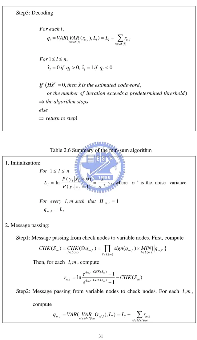
(44) Step3: Decoding For each l ,. ∑r. ql = VAR( VAR (rm ,l ), Ll ) = Ll +. m ,l m∈M ( l ). m∈M ( l ). For 1 ≤ l ≤ n, xˆl = 0 if ql > 0, xˆl = 1 if ql < 0 If ( Hxˆ T = 0, then xˆ is the estimated codeword , or the number of iteration exceeds a predetermined threshold ) ⇒ the algorithm stops else ⇒ return to step1. Table 2.6 Summary of the min-sum algorithm 1. Initialization: For 1 ≤ l ≤ n L l = ln. P ( yl xl = 0) P ( y l x l = 1). =. 2. σ. 2. For every l , m such that H. y l , where σ. m ,l. 2. is the noise variance. =1. q m ,l = L l. 2. Message passing: Step1: Message passing from check nodes to variable nodes. First, compute. CHK ( S m ) = CHK (⊕q m ,l ′ ) = l ′∈L ( m ). ∏. l ′∈L ( m ). sign(q m ,l ′ ) × MIN { q m ,l ′ } l ′∈L ( m ). Then, for each l, m , compute rm ,l = ln. e e. qm , l + CHK ( S m ). −1. qm , l −CHK ( S m ). −1. − CHK ( S m ). Step2: Message passing from variable nodes to check nodes. For each l, m , compute. q m ,l = VAR( VAR (rm ',l ), Ll ) = Ll + m '∈M ( l ) \ m. 31. ∑r. m ',l m '∈M ( l ) \ m.

(45) Step3: Decoding For each l , ql = VAR( VAR (rm ,l ), Ll ) = Ll + m∈M ( l ). ∑r. m ,l m∈M ( l ). For 1 ≤ l ≤ n, xˆl = 0 if ql > 0, xˆl = 1 if ql < 0 If ( Hxˆ T = 0, then xˆ is the estimated codeword , or the number of iteration exceeds a predetermined threshold ) ⇒ the algorithm stops else ⇒ return to step1. 32.

(46) Chapter 3 A New Structure for Low-Density Parity-Check Code Using the Difference Family. In this chapter, we will partition the discussion into two sections. In section 3.1, an introduction to the difference family and the construction of an irregular quasi-cyclic code based on this concept will be discussed. In section 3.2, we will propose a new structure of the low-density parity-check code, and expecting the new structure to bring performance improvement.. 3.1 The Difference Family In [5], a concept using the difference family to construct an irregular quasi-cyclic code with a Tanner graph free of 4-cycle was introduced. A difference family is an arrangement of a group of v elements, such as Z v , into not necessarily disjoint subsets of equal size which meet certain difference requirements. More precisely: Definition 1: The t γ -element subsets of the group Z v , D1 , D2 ,..., Dt with. Di = {d i ,1 , d i , 2 ,..., d i ,γ }. form a. (v, γ , λ ). 33. difference family if the difference.

(47) (d i , x − d i , y ) mod v , (i = 1, 2,..., t ; x, y = 1, 2, ..., γ , x ≠ y ) give each nonzero element of Z v exactly λ times. For example, the subsets D1 = {1, 2, 5} , D2 = {1, 3, 9} of Z 13 form a (13,3,1) difference family with differences From D1 : 2 − 1 = 1 , 1 − 2 = 12 , 5 − 1 = 4 , 1 − 5 = 9 , 5 − 2 = 3 , 2 − 5 = 10 From D2 : 3 − 1 = 2 , 1 − 3 = 11 , 9 − 1 = 8 , 1− 9 = 5 , 9 − 3 = 6, 3 − 9 = 7 . In this work where the difference families with λ = 1 allows the design of codes free of 4-cycles. For an irregular quasi-cyclic code, define the column weight distribution of a length vl rate l − (1 / l ) code as the vector W = [ w1 , w2 ,..., wl ] , where w j is the column weight of the columns in the j th circulant. Denote that wmax is the maximum column weight of the parity-check matrix H wmax = max{w1 , w2 ,..., wl } .. (3.1). To construct an irregular quasi-cyclic code with length vl and rate l − (1 / l ) , so that its parity-check matrix H = [a1 ( x), a 2 ( x),..., al ( x)]. has a weight distribution. W = [ w1 , w2 ,..., wl ] , l sets D1 , D2 ,..., Dl of a (v, γ ,1) difference family with. γ ≥ wmax , and a j (x) can be defined using w j of the elements of D j as a j ( x) = x. d j ,1. +x. d j,2. + ... + x. d j ,w j. .. (3.2). To ensure that the code can be encoded, x v − 1 must be divisible by at least one of the a j (x) . For a regular code, all of the elements in each set are included in each circulant, while for an irregular code the choice of which elements in the set to use is arbitrary. The row weight, ρ , of the parity-check matrix is constant, and given by. 34.

(48) l. ρ = ∑ wi .. (3.3). i =1. To demonstrate that the quasi-cyclic codes are free of 4-cycles we need a well known result of the difference families.. Lemma 3.1 [5]: A pair of elements from Z v occur together exactly λ times in the set of translates of every set in a (v, γ , λ ) difference family.. Lemma 3.2: The codes of construction by using difference families have Tanner graphs free of 4-cycles. Proof: Follows from the choice of λ = 1 . First consider the regular case. Each column of H = [a1 ( x), a 2 ( x),..., al ( x)] is a translate of one of the sets D j in the difference family. To show that there can be no 4-cycles in H , we need to show that no two columns of H can have a nonzero entry in the same two rows, which is equivalent to requiring that two elements of Z v can occur together in at most one of all the translates of the sets in the difference family. Since two elements occur together in exactly λ translates, we need only choose λ = 1 to avoid 4-cycles. The argument follows naturally in the irregular construction. Since only w j of the elements in a given set of the difference family will be taken, removing elements from the set of translates will keep it free of 4-cycles.. 3.2 The Proposed Structure of LDPC Code. According to section 3.1, we can use difference family to construct an irregular quasi-cyclic code free of 4-cycles. In the following section we will describe the construction we wish to propose for LDPC codes using these difference families. Below is our proposed structure of the parity-check matrix H,. 35.

(49) ⎡A H =⎢ 1 ⎣ B1. A2. ... Al −1. B2. ... Bl −1. 0⎤ . Bl ⎥⎦. (3.4). where A1 , A2 ,..., Al −1 , B1 , B2 ,..., and Bl are all v × v circulant matrices. The code length is vl and the code rate is ( 1 −. 2 ). We can use the difference families to l. determine the polynomials of each of the circulant matrix ai ( x) and b j ( x), where. i ∈ {1,2,..., l − 1} and j ∈ {1,2,..., l} , just as the quasi-cyclic code. In order to avoid any 4-cycles in the new structure of the parity-check matrix, we provide a new difference family to solve this problem. First, construct two (v, γ ,1) difference families Family A and Family B and combine the two families to form a new difference Family C which are needed to add the following two constraints. Constraint 1: The differences [( a i , x − a i , y )mod v ] and [( bi , x − bi , y )mod v ], where i = 1,2,..., l − 1; x, y = 1,2,..., γ , x ≠ y , give each element, can not be the same. Constraint 2: The differences [( a i , x − a j , y )mod v ] and [( bi , x − b j , y )mod v ], where i, j = 1,2,..., l − 1, i ≠ j; x, y = 1,2,..., γ , give each element, can not be the same. More precisely, if a parity-check matrix is 4-cycles free, it represents that no two columns of H can have a nonzero entry in the same two rows. Suppose the new circulant matrix is C i = [ Ai , Bi ]T where i ∈ {1,2,..., l} . Constraint 1 is added to avoid the case where any two columns of C i have a nonzero entry in the same two rows. Constraint 2 is added to avoid the case where a column of C i , i ∈ {1,2,..., l} and another column of C j , j ∈ {1,2,..., l} , i ≠ j have a nonzero entry in the same rows. For example, the subsets from the difference Family A are A1 = {3,7} and A2 = {1,6} , and the subsets from the difference Family B are B1 = {1,7} , B 2 = {2,3}. and B3 = {4,6} of Z 13 , which form a new (13,2,1) difference family C. The differences from Constraint 1: 36.

(50) From A1 : 3 − 7 = 9 , 7 − 3 = 4 From B1 : 1 − 7 = 7 , 7 − 1 = 6 From A2 : 1 − 6 = 8 , 6 − 1 = 5 From B 2 : 2 − 3 = 12 , 3 − 2 = 1 . The differences from Constraint 2: From A1 and A2 : 3 − 1 = 2 , 3 − 6 = 10 , 7 − 1 = 6 , 7 − 6 = 1 From B1 and B 2 : 1 − 2 = 12 , 1 − 3 = 11 , 7 − 2 = 5 , 7 − 3 = 4 . Regarding the encoding for the new structure, suppose that two of the circulant matrices Al −1 and Bl are invertible, we can derive two generator matrices in the following systematic forms. G 1 systematic. ⎡ ⎢ = ⎢ I v (l − 2) ⎢ ⎢ ⎣⎢. ( A l−−11 A1 ) T ⎤ ⎥ ( A l−−11 A 2 ) T ⎥ = I v (l − 2)G 1 ⎥ ... ⎥ ( A l−−11 A l − 2 ) T ⎦⎥. ⎡ ⎢ = ⎢ I v ( l −1 ) ⎢ ⎢ ⎣⎢. ( B l− 1 B 1 ) T ⎤ ⎥ ( B l− 1 B 2 ) T ⎥ = I v ( l −1 ) G 2 . ⎥ ... ⎥ ( B l− 1 B l − 1 ) T ⎦⎥. [. ]. (3.5). and. G 2 systematic. [. ]. (3.6). Let c = [d , p1 , p 2 ] denote the codeword of the proposed parity-check matrix where d is the message bits with length v(l − 2) , and p1 and p 2 combined are the parity bits, each having the same length v . The encoding procedure is partitioned into two steps.. Encoding Step1: We can use the generator matrix G1 to get the parity bits p1 . That is p1 = d × G1 .. (3.7). Then, combine the parity bits p1 with the message bits d to form an intermediate codeword c ′ where c ′ = [d , p1 ] .. Encoding Step2: The last parity bits p 2 can be derived from the generator matrix 37.

(51) G 2 and the intermediate codeword c ′ . That is p 2 = c′ × G2 .. (3.8). In fact, the encoding procedure for the proposed structure is very similar to the quasi-cyclic code discussed in section 2.3. The parity bits p1 can be generated with linear complexity by using a shift register of size v(l − 2) while encoding of the random codes is via matrix multiplication. For example, encoding of the Encoding Step1 requires vα 1 binary operations, α 1 is one less than the column weight of G1 , while matrix multiplication requires v[2v(l − 2) − 1] binary operations. Similarly, the parity bits p 2 can also be obtained by using a shift register of size v(l − 1) that needs vα 2 binary operations to complete the computation, where α 2 is one less than the column weight of G 2 . Since the encoding complexities of Encoding Step1 and Encoding Step2 are linear functions of to the code length, so is the total encoding complexity of the proposed structure which can be implemented by shift register and some combinatory logic.. 38.

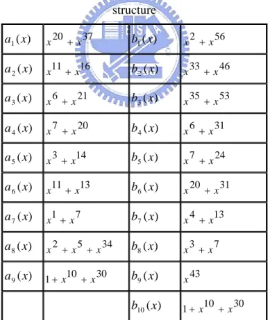
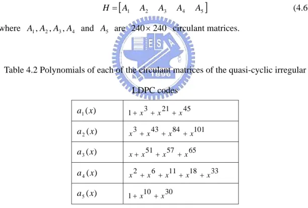
(52) Chapter 4 Simulation Results. In the beginning of this chapter, we will make a comparison of error correction performances by using some different structures of parity-check matrices such as irregular quasi-cyclic code, randomly constructed code and the proposed structure irregular code. Then, we will make a comparison of error correction performances by using some different decoding algorithms such as sum-product algorithm, min-sum based algorithm and min-sum algorithm. In the end, we will furthermore analyze the finite-precision effects on the decoding performance, and decide proper finite word lengths of variables considering tradeoffs between the performance and the hardware cost. Before proceed to the following simulation, some parameters should be described here: 1: The polynomials of each of the circulant matrices of the proposed LDPC code structure are shown in Table 3.1. Three proposed structures of irregular LDPC codes have been constructed. When the rate is 2/3 and code length is 720 with degree distribution W=[4, 4, 4, 4, 5, 3], the parity-check matrix is of the form ⎡A H =⎢ 5 ⎣ B5. A6. A7. A8. A9. B6. B7. B8. B9. 0 ⎤ B10 ⎥⎦. (4.1). where A5 , A6 ,..., A9 , B5 , B6 ,..., B9 and B10 are 120 × 120 circulant matrices. When the rate is 3/4 and code length is 960 with degree distribution W=[4, 4, 4, 4, 4, 4, 5, 3], 39.

(53) the parity-check matrix is of the form ⎡A H =⎢ 3 ⎣ B3. A4. A5. A6. A7. A8. A9. B4. B5. B6. B7. B8. B9. 0 ⎤ B10 ⎥⎦. (4.2). where A3 , A4 ,..., A9 , B3 , B 4 ,..., B9 and B10 are 120 × 120 circulant matrices. When the rate is 4/5 and code length is 1200 with degree distribution W=[4, 4, 4, 4, 4, 4, 4, 4, 5, 3], the parity-check matrix is of the form ⎡A H =⎢ 1 ⎣ B1. A2. A3. A4. A5. A6. A7. A8. A9. B2. B3. B4. B5. B6. B7. B8. B9. 0 ⎤ B10 ⎥⎦. (4.3). where A1 , A2 ,..., A9 , B1 , B 2 ,..., B9 and B10 are 120 × 120 circulant matrices.. Table 4.1 Polynomials of each of the circulant matrices of the proposed LDPC code structure 20. +x. 37. b1 ( x). x. 11. +x. 16. b2 ( x ). x. a1 ( x). x. a 2 ( x). x. a 3 ( x). x. a 4 ( x). x. a 5 ( x). x. a 6 ( x). x. a 7 ( x). 1 7 x +x. a8 ( x). x. a 9 ( x). 1+ x. 2. 33. +x. 46. 35. +x. 53. 6. +x. 21. b3 ( x). x. 7. +x. 20. b4 ( x ). x. 3. +x. 14. b5 ( x). x. b6 ( x ). x. b7 ( x ). x. b8 ( x). x. b9 ( x). x. b10 ( x). 1+ x. 11. 2. +x. +x 10. 13. 5. +x. +x. 34. 30. 56. +x. 6. +x. 31. 7. +x. 24. 20. +x. 31. 4. +x. 13. 3. +x. 7. 43 10. +x. 30. 2: The polynomials of each of the circulant matrices of the irregular quasi-cyclic codes are shown in Table 3.2. Three quasi-cyclic irregular LDPC codes have been 40.

(54) constructed. When the rate is 2/3 and code length is 720 with degree distribution W=[4, 5, 3], the parity-check matrix is of the form H = [A3. A5 ]. A4. (4.4). where A3 , A4 and A5 are 240 × 240 circulant matrices. When the rate is 3/4 and code length is 960 with degree distribution W=[4, 4, 5, 3], the parity-check matrix is of the form H = [ A2. A3. A5 ]. A4. (4.5). where A2 , A3 , A4 and A5 are 240 × 240 circulant matrices. When a rate 4/5, code length is 1200 with degree distribution W=[4, 4, 4, 5, 3], the parity-check matrix is of the form H = [A1. A2. A3. A5 ]. A4. (4.6). where A1 , A2 , A3 , A4 and A5 are 240 × 240 circulant matrices.. Table 4.2 Polynomials of each of the circulant matrices of the quasi-cyclic irregular LDPC codes 3. +x. 21. +x. 45. +x. 43. +x. 84. +x. a1 ( x). 1+ x. a 2 ( x). x. a 3 ( x). x+x. a 4 ( x). x. a 5 ( x). 1+ x. 3. 2. 51. +x 10. +x. 6. 57. +x. 11. +x. +x. +x. 101. 65 18. +x. 33. 30. 3: The randomly constructed codes are derived from [14] and [15], and they have a regular column weight of four with similar parameters. This means that for a rate of 2/3 and code length of 720 with a random structure, the column weight is four and the averaged row weight is twelve. Similarly, for a rate of 3/4 and code length of 960 with. 41.

(55) a random structure, the column weight is four and the average row weight is sixteen. Finally, for a rate of 4/5 and code length of 1200 with a random structure, the column weight is four and the average row weight is twenty. 4: For the decoding algorithm, we adopt the sum-product algorithm, min-sum based algorithm and min-sum algorithm. The maximum iteration loops = 10 . 5: We use the AWGN channel and BPSK modulation method as our test environment.. 4.1 Floating-Point Simulations Figures 4.1-4.3 show the error correction performance for different structures of the parity-check matrix that use the sum-product algorithm for iterative decoding. We can see that in Figures 4.1-4.3, using the proposed structures of the parity-check matrix, the decoding performance is the best, compared to the irregular quasi-cyclic codes and randomly constructed codes. Figures 4.4-4.6 show the error correction performance for different decoding algorithms such as the sum-product algorithm, the min-sum based algorithm and the min-sum algorithm. In the simulations and figures the proposed parity-check matrix structures assume some different code lengths and code rates. We can see that in Figures 4.4-4.6, the decoding performances are almost the same for the sum-product and the min-sum based algorithms combined with iterative decoding. As shown, the min-sum algorithm has the worst performance of all the compared algorithms. This is due to the fact that the min-sum algorithm in the check node update is an approximate form and using the approximation will cause a performance penalty of about 0.5dB.. 42.