一個基於花與葉片之植物辨識系統

國

立

交

通

大

學

多媒體工程研究所

碩

士

論

文

一 個 基 於 花 與 葉 片 之 植 物 辨 識 系 統

A Plant Recognition System Based on Leaf and Flower

研 究 生：楊志鴻

指導教授：陳玲慧 教授

一個基於花與葉片之植物辨識系統

研究生：楊志鴻

指導教授：陳玲慧 博士

國立交通大學多媒體工程研究所

摘要

本篇論文中我們提出一個基於花與葉片之植物辨識系統，針對台

中都會公園的植物，利用照相手機所拍攝的花朵影像及葉片影像進行

辨識。辨識系統共分為三大部分。第一部分為花朵辨識系統，總共使

用了花朵的十四種特徵，包含三種外型以及十一種顏色的特徵。為了

從複雜的背景中擷取出花朵的部分，我們提出了一個快速自動化切割

物體的方法，並藉由使用者互動方式擷取出花朵部分。第二部份為葉

片辨識系統，共使用了葉片的五個外型特徵。葉片自動辨識系統分為

兩個階段，第一階段先將與輸入影像差異大的種類刪除，而第二階段

依據第一階段過濾後的數種名單進行最後的辨識動作。系統的第三部

份為針對開花植物中結合花朵以及葉片的辨識系統。首先，分別先將

花朵以及葉片進行辨識。接著，我們提出了一個有效結合花朵以及葉

A Plant Recognition System Based on Leaf and

Flower

Student: Chih-Hung Yang

Advisor: Dr. Ling-Hwei Chen

Institute of Multimedia Engineering

National Chiao Tung University

Abstract

In this thesis, we propose a plant recognition system based on leaf and flower

images. The images are taken in the Taichung Metropolitan Park by the camera

mobile phone. There are three parts in the recognition system: flower, leaf, and

combination of flower and leaf. In the flower recognition part, 14 features of flowers,

including 3 shape features and 11 color features, are used. We propose a fast and

automatic object segmentation method and combine user’s interaction to extract the

flower region. In the leaf recognition part, 5 shape features are extracted. A two-stage

approach is provided for automatic leaf recognition. Firstly, some impossible species

are pruned according to the first three features. Next, the remaining species are tested

of leaf and flower images are recognized respectively. Then, an effective method is

presented to do recognition by combining the recognition results of leaf and flower.

According to experimental results, the combining recognition part can improve the

誌 謝

這篇論文的完成，首先要感謝指導教授陳玲慧博士，在這兩年碩

士生涯中，老師在課業上和生活上給予的指導與關心，讓我在交大學

到的不僅是學業上的知識，還有更多做人做事的道理。另外，要感謝

李建興學長給予的建議以及指導。此外，感謝口試委員鍾國亮教授、

張隆紋教授以及李遠坤教授於口試中給予的指導與建議。

接著，要謝謝實驗室一起生活一起奮鬥的夥伴們，博士班的學長

姐們，民全、萓聖、文超、惠龍、俊旻、占和、盈如以及芳如，還有

畢業的學長姐們，立人、信嘉、偉全、子翔和薰瑩，以及同屆的同學，

益成、明旭與志達，和學妹佳瑄，因為有大家的陪伴，讓我兩年的碩

士生涯過得充實又豐富。

此外，還要感謝資工系壘的隊友們，謝謝你們讓我有機會能在壘

球場上盡情地發揮，並且一起努力拿到校外比賽，瘋竹盃冠軍、北資

盃亞軍的佳績，為我碩士生涯增添許多色彩。

最後，要感謝我最重要的家人：爸爸、媽媽、姐姐、妹妹以及香

鈞，在我的研究生涯中給予各種生活上的協助，讓我能專心於研究

中。謹以此篇論文獻給我的父母，以及所有關心我、鼓勵我的朋友們。

TABLE OF CONTENTS

摘要... i

Abstract... ii

誌 謝... iv

TABLE OF CONTENTS...v

LIST OF FIGURES ... vii

LIST OF TABLES... ix

CHAPTER 1 INTRODUCTION...1

1.1 Motivation...1

1.2 Previous work ...1

1.3 Organization of the Thesis ...4

CHAPTER 2 IMAGE DATABASE...5

2.1 Flower Image Database...5

2.2 Leaf Image Database...7

CHAPTER 3 PROPOSED system ...10

3.1 Flower Recognition Method ...10

3.1.1 Preprocessing for Flower ... 11

3.1.1.1 Flower Area Location by User Interaction...12

3.1.1.2 Spatial Regions Merging...13

3.1.1.3 Small Regions Merging ...15

3.1.1.4 Flower Region Selection and Extraction ...17

3.1.2 Feature Extraction for Flowers ...18

3.1.2.1 Shape Information...18

3.2.1.1 Gray-scale Transformation...24

3.2.1.2 Bi-level Transformation ...25

3.2.1.3 Principle Component Transformation...27

3.2.2 Feature Extraction for Leaf...28

3.2.2.1 Shape Information...29

3.2.3 Leaf Recognition...30

3.2.3.1 Preliminary Stage...30

3.2.3.2 Essential Stage ...38

3.3 Combining Recognition Method...38

3.3.1 Combining Recognition ...39

CHAPTER 4 EXPERIMENTAL RESULTS...41

CHAPTER 5 CONCLUSION...50

LIST OF FIGURES

Fig. 1 Images of 24 distinct flowers ...…...…..……..……….….6 Fig. 2 Some examples of flowers with different colors in the same species ...7 Fig. 3 24 distinct leaves corresponding to the blooming flowers shown in Fig. 1 ..8 Fig. 4 Other 24 species collected with leaves only ………...9 Fig. 5 The flow chart of the proposed method for flower recognition …….…….11 Fig. 6 The flow chart of the preprocessing steps of flower recognition ….……...12 Fig. 7 An example of determining flower area location by user interaction. (a)

Original image. (b) The rectangle is drawn by user …..………..13 Fig. 8 Two Sobel operators for Gx and Gy …..………..…………..…...14

Fig. 9 An example of the preprocessing results. (a) The original image. (b) The result of small region merging. (c) The petal and stamen region selected by user. (d) The stamen region …...18 Fig. 10 An example of the preprocessing results with the colors of petals and

stamens similar. (a) The original image. (b) The result of small region merging. (c) Flower region selected by user. (d) The stamen region …...18 Fig. 11 The HS space divided into 12x6 cells ..………...22 Fig. 12 The flow chart of the proposed method for leaf recognition ...……….…...24 Fig. 13 The flow chart of the preprocessing steps of leaf recognition …...….……24 Fig. 14 An example of gray-level transformation. (a) Original image. (b) Gray-level

image …..………...……….………...25 Fig. 15 An example of bi-level transformation. (a) Gray-level image. (b) Bi-level

image …...………....26 Fig. 16 A special case of bi-level transformation. (a) A bi-level image. (b) The result of first thresholding. (c) The result of second thresholding …...27 Fig. 17 An example of principle component transformation. (a) The boundary of a

leaf image and its principle component. (b) The transformed boundary of a leaf image ………..28 Fig. 18 The bounding box of a leaf ………..29 Fig. 19 The flow chart of leaf recognition method ………..30 Fig. 20 The ranges of three features. (a) The ranges of AR. (b) The ranges of RR. (c)

The ranges of SR ……….………37 Fig. 21 The flow chart of the proposed method for combining recognition……….39

recognition results. (c) The retrieved information of the query image. (d) Combining recognition results ….………...48

LIST OF TABLES

Table 1 The ranges of AR, RR and SR of every plant species in our database ……31 Table 2 Performance on our flower database ………...42 Table 3 Performance comparison between our method and Zou-Nagy’s method

using Zou-Nagy’s database ……….43 Table 4 Performance on our leaf database by returning Top-5 images ..…………..44 Table 5 Performance on our leaf database by returning Top-5 species ..…………..44 Table 6 Performance comparison between our method and Lee-Chen’s method

using Lee-Chen’s database ………….……….45 Table 7 Performance comparison between our method and Saitoh-Kaneko’s method

using the same numbers of Saitoh-Kaneko’s database ...………….……....45 Table 8 Performance comparison ………...…..…46

CHAPTER 1

INTRODUCTION

1.1 Motivation

When wandering around the field or park, we can find out many plants. If there

are no signs for the plants, we can not know their names on the instant. Although we

can try to identify the names of plants by looking up guide books for plant, or

browsing web pages on the Internet through keywords searching, it is inconvenient

and difficult to look for the name of specific plant. Since the camera mobile phone has

been widely used for most people, it would be very useful and convenient if we can

use the plant recognition system to identify the plants directly based on photograph by

camera mobile phone.

1.2 Previous work

Plants are basically classified according to their shapes, colors and structures of

their leaves and flowers. It is very difficult for us to recognize the plant without any

knowledge of botany. In this thesis, we proposed a plant recognition system based on

a photograph. It is a necessary step to extract a flower region or a leaf region of

interest from the background for recognition. However, it is more difficult to achieve

To avoid this difficulty, Saitoh and Kaneko [1, 2] used a piece of black cloth (or

black paper) under the flower and leaf when they took photographs. To separate the

background, they used K-means algorithm [3] for clustering in RGB space and then

removed the background region. Then, they proposed 21 features, including 10

features of flower and 11 features of leaf in recognition phase, and received a high

accuracy rate above 95%. Nevertheless, it is inconvenient and laborious to photograph

flowers and leaves with a piece of back cloth and the direction of leaf should be fixed.

Chen [4] proposed an automatic segmentation algorithm for natural images.

Considering from human vision, they transformed RGB color space into CIELab

color space [5-6]. Then, they also used K-means algorithm [3] to classify all colors in

the image and proposed a two-stage method to segment regions by colors. However,

the segmentation takes a lot of time and is impractical.

Zou and Nagy [7] used the rose curve which was defined by the Italian

mathematician Guido Grandi for segmentation. Firstly, they used a rose curve model

fitting on the initial segmented flower region and allowed interactive adjusting by user

to fit the real flower region. When adjusting the curve of the flower, the system would

Saitoh et al. [8] proposed an automatic method for extracting flower region and

recognition. For extracting the flower boundary, they used the well-known method

proposed by Mortensen and Barrett called Intelligent Scissors (IS) [9]. Pictures were

taken with macro mode setting F value from F2.8 to F3.5. They used 10 features for

flower recognition and received high accuracy above 90%. However, there are some

limitations such as the position of the flower must be in the center of the photograph

and be well focused, with background defocused.

Wang et al. [10] proposed a two-stage approach for leaf image retrieval by using

shape features such as centroid-contour distance (CCD) curve, eccentricity, and angle

code histogram (ACH). The two-stage approach can achieve a performance

comparable to an exhaustive search, but with a much reduced computational

complexity. The average recall rate is 38.1% for 20 return images.

Lee and Chen [11] proposed a classification method for leaf images. They

proposed 5 region-base features for leaf recognition. The accuracy rate is 82.33% and

the recall rate is 48.2% for 10 return images. However, the leaf should be put on the

light panel and the direction of leaf must be fixed when taking picture of leaf. It is

also inconvenient for users to get leaf image by this way.

In this thesis, we propose three methods in our recognition system, including

method is provided for flower segmentation which utilizes user’s interaction to

eliminate the limitations of photographs and to get a correct flower region of interest.

Then, we adopt 14 various features including 3 for shapes and 11 for colors for

recognition. Secondly, a two-stage automatic region-base method is used for leaf

recognition. We use some techniques to remove noises and to solve rotation problem.

Then, we can get the leaf region of interest and adopt 5 shape features for recognition.

Thirdly, we propose a combining recognition method based on a pair of images of

flower and leaf. The features of flower and leaf are extracted respectively by the steps

described above. Then, we combine the features of flower and leaf for recognition.

Experimental results show that the combining recognition method can get higher

accuracy rate than using only flower or leaf.

1.3 Organization of the Thesis

This thesis is composed of five chapters. In Chapter 1, the motivation and

previous works are introduced. Chapter 2 describes the database images including

flower and leaf images used in the study. The proposed recognition method is

CHAPTER 2

IMAGE DATABASE

The image database consists of flower images and leaf images taken in the

Taichung Metropolitan Park by camera mobile phone. Pictures were taken with macro

mode and an aperture value 2.8F. Camera mobile phone used is Nokia N82. All

images are re-scaled to the same size, 320x240 pixels, before recognition.

2.1 Flower Image Database

The flower image database consists of 684 flower images with 24 species. Each

of the flower images will be selected as the testing data, and the remaining 683

images are then used for database. There are at least 20 images for each species and

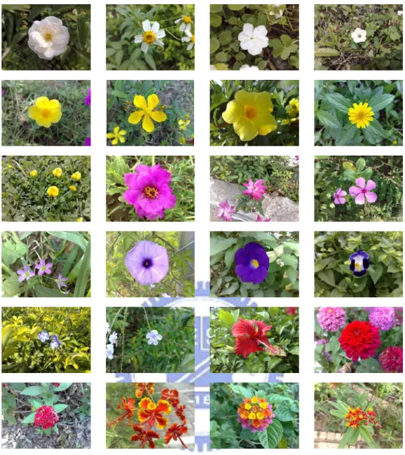
the images are taken from natural scene by camera mobile phone. Fig. 1 shows 24

species of flowers in our database. Several images contain multiple, tiny, overlapping

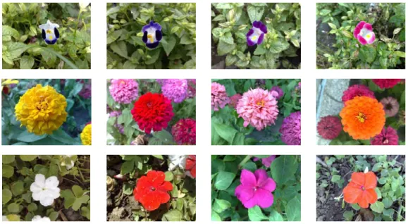
flowers. Some flowers have different colors in the same species as shown in Fig. 2.

Fig. 2 Some examples of flowers with different colors in the same species.

2.2 Leaf Image Database

Leaves are usually clustered, so it is difficult to extract a leaf automatically from

a natural image. As a result, we plucked a leaf and put it on a piece of white paper,

and took the picture of the leaf with camera mobile phone. Thus, leaf images can be

obtained without complex background.

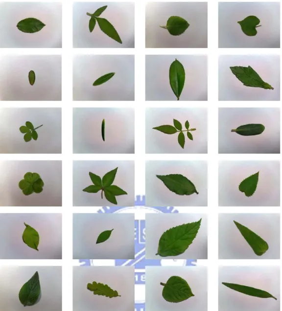
The leaf image database consists of 1920 leaf images from 48 species. Each

species includes 40 images; the 20 images of them are used for database images and

the others are used for testing images. Fig. 3 shows the 24 species of the leaves, which

have corresponding blooming flowers shown in Fig. 1. For the other 24 species, we

only collect the leaves as shown in Fig. 4. For robustness, we plucked 15 to 20 leaves

CHAPTER 3

PROPOSED SYSTEM

In this thesis, we propose a recognition system for plants. The plant recognition

system has three functions which are flower recognition, leaf recognition and

combining recognition. When a user only input a flower image or a leaf image, this

system can recognize the query image and return the possible species to the user.

When the user input a pair of images including the flower and the leaf, this system

can get better result than only using a flower image or a leaf image. Details will be

described in the following sections.

3.1 Flower Recognition Method

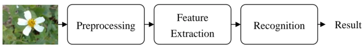
Fig. 5 shows the flow chart of the proposed method for flower recognition. The

whole process consists of three major phases: preprocessing, feature extraction, and

recognition. In the preprocessing phase, the proposed method provides a

semi-automatic technique to find out the flower region. In the feature extraction phase,

3 shape features and 11 color features are extracted for recognition. In the recognition

3.1.1 Preprocessing for Flower

Extracting a flower region from the background is a necessary step for flower

recognition. In order to extract the flower region as correctly as possible, the proposed

method provides a semi-automatic technique to locate the flower area. Because the

flower always has the significant color distinct from the leaves, we can use color

information to segment the region of the flower. Here the K-means algorithm is used

to find the dominant colors of the flower image. According to the statistics, there are

averagely fifty thousand colors in each flower image of our database. It costs

extensive computation time to extract the dominant colors form fifty thousand colors

by K-means. In order to speed up the process time, we first gather the nearby pixels

with the similar colors and merge them into small regions. After that, we can reduce

the colors of a flower image from fifty thousand to hundreds. Next, we use an

automatically segment method proposed in [4] to determine the dominant colors by

K-means and then replace the colors of small regions with the dominant colors. Then,

the region growing technique is applied to merge those neighboring small regions of Result Preprocessing Feature

Extraction Recognition

the same color. Finally, the flower region can be extracted by user selection based on

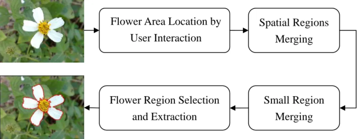
the segmentation results. Fig. 6 shows the flow chart of the preprocessing steps.

3.1.1.1 Flower Area Location by User Interaction

In order to reduce the limitations of input images and to extract the correct

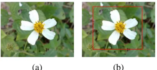
flower region, an interactive method is provided. At first, a rectangle is drawn by

user’s mouse click to bind an interested flower. Fig. 7 shows an example of

determining flower area location by user interaction. We called the region within the

rectangle as the object region. After the flower area is located, we present a

semi-automatic segment method to extract the flower region. The details are described

in the following subsections.

Flower Area Location by User Interaction

Spatial Regions Merging

Small Region Merging Flower Region Selection

and Extraction

(a) (b)

Fig. 7 An example of determining flower area location by user interaction. (a) Original image. (b) The rectangle is drawn by user.

3.1.1.2 Spatial Regions Merging

Most of flowers have the significant color distinct from leaves, therefore the

color information is used to do segmentation and then we can extract the flower

region by user interaction. To reduce the number of colors in the image without losing

the important spatial information of colors, we first gather the nearby pixels with

similar colors in the object region into a small region. Note that the differences of

nearby pixels are below a threshold, we called them have the similar colors. The

threshold is determined by edge detection described as following:

To estimate edge points in the object region, we apply Sobel operators (see Fig.

8). The gradient magnitude G for pixel (x, y) with color value Px, y is defined as

(

) (

)

(

) (

)

Gx is the magnitude of horizontal gradient and Gy is the magnitude of vertical one.

-1 0 1

-2 0 2

-1 0 1

-1 -2 -1

0 0 0

1 2 1

Fig. 8 Two Sobel operators for Gx and Gy

We compute the gradient magnitudes for R, G, and B channels. Next, we take the

maximum value of three gradient magnitudes for each pixel to form another image.

And then the Otsu’s method [12] is applied to the image to get a binary image. Finally,

we can get all edge points from the binary image easily.

According to the edge detection result, the percentage of edge points and smooth

areas can be estimated. Then, we define four color differences: (i) the difference of R

channel, (ii) the difference of G channel, (iii) the difference of B channel, (iv) the total

difference of R, G and B channels which is defined as diff= (r₁−r₂)2+(g₁−g₂)2+(b₁−b₂)2. We calculate the four differences to the 8 neighbors for each pixel in the object region.

After that, we compute the four accumulated histograms and calculate the cumulative

distribution function (CDF), respectively. In each CDF, the difference value at the

same percentage as the smooth areas percentage is considered as threshold. Based on

color of the component is decided by the average color of all pixels in the component.

Each time when the component meets a new point, the four color differences between

the average color of the component and the new point will be calculated. If one of

these differences exceeds the threshold, the new point will be regarded as a starting of

a new component; otherwise, it will be included to the component and the process

will continue. After the process, there will be hundreds of connected component

regions with different sizes. Since most of the connected components are small, we

should merge those small regions. Thus, the next process will be used to merge small

regions. It will first find the dominant colors for these regions based on K-means and

replace the colors of these regions with those found dominant colors. The step is used

to speed up the merging process.

3.1.1.3 Small Regions Merging

In this section, we will apply a modified K-means method to merge small regions.

Before describing this method, we will introduce the used color space. Since the RGB

color space is perceptually non-linear to human vision system, the RGB color space

will be transformed into CIELab color space [5-6] based on ITU-R Recommendation

, 950227 . 0 119193 . 0 019334 . 0 072169 . 0 715160 . 0 212671 . 0 180423 . 0 357580 . 0 412453 . 0 ' ' ' ⎥ ⎥ ⎥ ⎦ ⎤ ⎢ ⎢ ⎢ ⎣ ⎡ ⎥ ⎥ ⎥ ⎦ ⎤ ⎢ ⎢ ⎢ ⎣ ⎡ = ⎥ ⎥ ⎥ ⎦ ⎤ ⎢ ⎢ ⎢ ⎣ ⎡ B G R Z Y X

,

088754

.

1

/

'

000000

.

1

/

'

950456

.

0

/

'

⎪

⎩

⎪

⎨

⎧

=

=

=

Z

Z

Y

Y

X

X

After transforming the average color of each component to CIELab color space,

the modified K-means method is conducted. There is a significant drawback with the

traditional K-means algorithm; the K value cannot be adjusted after decided. Hence,

we use the concept from [4], that is, an “error threshold” is provided to decide the

suitable K. The average error after applying K-means method is defined as the

average color difference among the original colors and the colors of the results by

K-means. Firstly, we set K=2, and then the K-means method is applied. When the

average error is larger than the error threshold, K is increased and K-means method is (3) (2)

(5) (4)

our method, the error threshold is defined as 10% of the Lab color bandwidth. After

the step, the color of each pixel in the object region will be transformed to the nearest

dominant color. Then all neighboring pixels with the same dominant color are merged

into a region.

3.1.1.4 Flower Region Selection and Extraction

Based on the merging results, the object region can be segmented by dominant

colors as shown in Fig. 9(b). Since the system cannot automatically identify the

flower regions from these segment results, a way of utilizing the user interaction is

proposed. From Fig. 9(b), we can find that a flower is segmented to several regions.

To acquire the complete flower region, users can use mouse click to point out the

regions of the petal and stamen. After that, a flower region including the petal and

stamen regions can be extracted as shown in Figs. 9(c) and 9(d). Sometimes the

stamen color is so similar to the petal color, that the stamen region can not be

extracted. To treat this case, the stamen region is defined as the rectangular window

with the flower center as its center, and its area being 1/9 of the flower bounding box.

Fig. 10 shows an example of the preprocessing results with the colors of petals and

(a) (b) (c) (d) Fig. 9 An example of the preprocessing results. (a) The original image. (b) The segmentation results. (c) The petal and stamen region selected by user. (d) The stamen region.

(a) (b) (c) (d) Fig. 10 An example of the preprocessing results with the colors of petals and stamens similar. (a) The original image. (b) The segmentation results. (c) The flower region selected by user. (d) The stamen region.

3.1.2 Feature Extraction for Flowers

Color and shape are the most widely-used features for describing flowers. In this

thesis, 3 shape features and 11 color features are used for flower recognition. Parts of

these features were proposed by Hsu [13].

3.1.2.1 Shape Information

Firstly, the gravity center (gx, gy) of the flower region is computed as follows:

where N is the number of pixels in the flower region, xi and yi are the coordinates of

the ith pixel in the flower region. The distance between the flower center and each

pixel in the flower region is computed as follows:

. 1 , 2 2 N i ) g (y ) g (x di = i− x + i − y ≤ ≤

Without loss of generality, we let di be sorted in an increasing order. That is,

1 1 , 1 ≤ ≤ − ≤d₊ i N

d_{i i} . The CDD [10] is a set of distances from those points in the contour to the shape center. Then the three shape features are described as follows:

F(1): Sharpness. A ratio indicates the relevance sharpness of the petals to the

flower. It is computed as , (1) 90 10 CCD CCD F =

where CCD10 represents the average of the top one-tenth of the shortest CCD and

the and CCD90 represents the average of the top one-tenth of the largest CCD.

F(2): It represents the average of normalized distances computed from the flower

center to every point in the flower region. It is computed as , 1 ) (2 1

∑

where Di is the normalized distance defined as

⎪ ⎪ ⎩ ⎪ ⎪ ⎨ ⎧ ≤ < < − − ≥ = 10 90 10 10 90 10 90 , 0 , , , 1 R d R d R R R R d R d D i i i i i

and R represents the average distance computed from the pixels with d in the (7)

(8)

(9)

first 10% of dj and R90 is computed from the pixels with di in the last 10% dj: , 1 . 0 1 , 1 . 0 1 9 . 0 90 1 . 0 1 10

∑

∑

F(3): Roundness. The roundness represents the similarity between the shape of

petals and a circle. It is computed as

, 4 ) 3 ( ₂ L S F = π

where L is the perimeter of the flower and S is the area of the flower with 1

) 3 (

0< F ≤ . When F(3)is approximating to 1, it means that the shape of flower is

near a circle.

3.1.2.2 Color Information

The flower images are represented in the RGB model. Because flower images

are taken in different days and under various kinds of weather, the RGB values are

converted into the HSV (hue, saturation and value) values [14] in order to reduce the

illumination variation. Our features are taken by the primary, secondary and thirdly

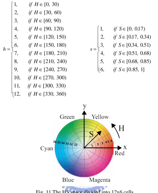
flower colors and the stamen color. Firstly, the H value is divided into 12 partitions

and the S value is divided into 6 partitions and there are totally 72 cells represented by (12) (11)

three dominant color cells appearing in the flower region. Then, the color features can

be summarized as

F(4): the h value of the color cell DC1,

F(5): the s value of the color cell DC1,

F(6): the probability of the color cell DC1,

F(7): the h value of the color cell DC2,

F(8): the s value of the color cell DC2,

F(9): the probability of the color cell DC2,

F(10): the h value of the color cell DC3,

F(11): the s value of the color cell DC3,

F(12): the probability of the color cell DC3,

Since the color of the stamen is also an important characteristic, we will compute

the dominant color of the stamen region. Let SC denote the dominant color cell in the

stamen region, then the color features of the stamen are defined as

F(13): the h value of the color cell SC.

F(14): the s value of the color cell SC.

Note that we have used the following equations to normalize the H and S values

⎪ ⎪ ⎪ ⎪ ⎪ ⎪ ⎪ ⎪ ⎩ ⎪ ⎪ ⎪ ⎪ ⎪ ⎪ ⎪ ⎪ ⎨ ⎧ ∈ ∈ ∈ ∈ ∈ ∈ ∈ ∈ ∈ ∈ ∈ ∈ = ) 360 0 [33 12 ) 330 0 [30 11 ) 300 270 [ 10 ) 270 240 [ 9 ) 240 210 [ 8 ) 210 0 [18 7 ) 180 0 [15 6 ) 150 0 [12 5 ) 120 0 [9 4 ) 90 0 [6 3 ) 60 30 [ 2 ) 30 0 [ 1 , H if , , H if , , H if , , H if , , H if , , H if , , H if , , H if , , H if , , H if , , H if , , H if , h ⎪ ⎪ ⎪ ⎪ ⎩ ⎪⎪ ⎪ ⎪ ⎨ ⎧ ∈ ∈ ∈ ∈ ∈ ∈ = ] 1 .85 0 [ 6 ) 85 0 68 0 [ 5 ) 68 0 51 0 [ 4 ) 51 0 34 0 [ 3 ) 34 0 17 0 [ 2 ) 17 0 0 [ 1 , S if , . , . S if , . , . S if , . , . S if , . , . S if , . , S if , s

Fig. 11 The HS space divided into 12x6 cells.

3.1.3 Flower Recognition

Before recognition, all features, F(i), are normalized to [0, 1] and represented by

f(i). In the recognition phase, we calculate the distances between the query image and

all flower images in the database. The distance disti, which is between the query

where fi(k) denotes the k-th feature value of the i-th database image, f(k) denotes the

k-th feature value of the query image. Then, flower recognition is accomplished using

the k-nearest neighbor algorithm. After that, the recognition system ranks the

distances and returns the Top-20 nearest neighbors. Then, the system gives scores to

each rank such as 1st = 20, 2nd = 19 …, respectively. Next, we sum up the scores of the

same species and compute the similarity. Finally, we rank the similarity and return the

flower images of possible species.

3.2 Leaf Recognition Method

The leaf recognition method is originally proposed by Huang [15]. Based on the

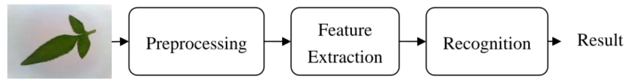
method, we do some improvement in leaf extraction and recognition rate. Fig. 12

shows the flow chart of the proposed method for leaf recognition. The whole process

consists of three major phases: preprocessing, feature extraction and recognition. In

preprocessing phase, we use some techniques to extract the leaf object. In the feature

extraction phase, five shape features are extracted for recognition. Then, we apply a

two-stage recognition based on the extracted features. The impossible species can be

pruned in the first stage. The second stage uses a similarity measure for the remaining

3.2.1 Preprocessing of Leaf

When we take picture of the leaf image, there could be some distortion

(including rotation, translation and scaling) and unbalanced light condition. Therefore,

we have to overcome these problems according to following five steps as shown in

Fig. 13. After that, the leaf object can be extracted and be normalized.

3.2.1.1 Gray-scale Transformation

image to a gray-level image. Each pixel is computed from the original image by , 3 ) , ( ) , ( ) , ( ) , (i j R i j G i j B i j gray = + +

where R(i, j), G(i, j) and B(i, j) denote the red value, green value and blue value at

pixel Pi, j. An example of gray-level transformation is shown in Fig. 14.

(a) (b)

Fig. 14 An example of gray-level transformation. (a) Original image. (b) Gray-level image.

3.2.1.2 Bi-level Transformation

To simplify the cost of computation, we transform the gray-level image to

bi-level image. Otsu’s method [12] is a classical method, which binarizes a gray-level

image to a binary image. The algorithm assumes that an image contains two classes of

pixels. It finds the optimum threshold separating the two classes so that their

within-class variance is minimal.

After using Otsu’s method to find the optimum threshold, the pixels are

separated into background area and leaf object area. The pixel with gray value in the

gray-level image larger than the threshold t be considered as background and set its (14)

gray value to 255; otherwise, it is regarded as the leaf object and set its gray value to 0.

An example of bi-level transformation is shown in Fig. 15.

(a) (b)

Fig. 15 An example of bi-level transformation. (a) Gray-level image. (b) Bi-level image.

By the above steps, we can extract the leaf objects correctly from most of the leaf

images. Some species of the leaf images can not be extracted successfully, because

the size of the leaf is too small or the color of the leaf is too light. Hence, the

following steps will solve this problem on the bi-level image (See Fig. 15(b)). Firstly,

the positions of the black pixels in the bi-level image are recorded. Next, we preserve

the pixels in the gray-level image according to the positions. Then, the Otsu’s method

is applied to these pixels on the gray-level image to do bi-level transformation. Fig. 16

is an example of this case. After bi-level transform, we can get a binary image. Based

(a) (b) (c) Fig. 16 A special case of bi-level transformation. (a) A gray-level image. (b) The

result of first thresholding. (c) The result of second thresholding.

3.2.1.3 Principle Component Transformation

We face another issue that the direction of the leaf images are various during

feature extraction. To solve this problem, we use the principle component to align the

image with the direction of maximum variance.

Let

Xk = (xk, yk) be the position of the k-th boundary point of a leaf pixel,

n = the number of boundary pixels.

We present the steps of principle component transformation as follows:

1. Compute the center point mx of the boundary pixels by

∑

2. Compute the covariance matrix

∑

3. Let V = (ei, ej) be the normalized associated eigenvector of the max eigenvalue of

θ . Note that V is the principle (15)

component of the boundary points.

4. Let the transformation matrix A be _⎥ ⎦ ⎤ ⎢ ⎣ ⎡ − θ θ θ θ cos sin sin cos .

5. Rotate the leaf with θ degree according to Y_k = A(X_k −m_x),

such that the principle component of the boundary points will coincide with the x-axis.

Fig. 17 shows an example of principle component transformation.

(a) (b)

Fig. 17 An example of principle component transformation. (a) The boundary of a leaf image and its principle component. (b) The transformed boundary of a leaf image.

3.2.2 Feature Extraction for Leaf

Note that most leaves have green color, the color information is improper for

recognition. According to the theory of plant taxonomy [16], external leaf

characteristics are important for identifying plant species. Thus, we use the shape

information of leaf for recognition. In this section, 5 shape features are used. We use a

rectangle enclosing the leaf, and call it as a bounding box, B, shown in Fig. 18. (17)

Fig. 18 The bounding box of a leaf.

3.2.2.1 Shape Information

L(1): Aspect Ratio (AR). The AR represents the ratio of the vertical length

(height) to horizontal length (width) of B. It is computed as . (1) B of width B of height L =

L(2): Rectangularity Ratio (RR). The RR represents the ratio of the area of the

leaf to the area of B. It is computed as . (2) B of area the leaf of area the L =

L(3): Sharpness Ratio (SR). The SR represents the ratio of the average of the top

one-tenth of the shortest CCD to the average of the top one-tenth of the largest CCD.

It is computed as . (3) 90 10 CCD CCD L =

L(4): UpAndDown Ratio (UDR). The UDR represents the ratio of the area of the

upper part to the area of lower part of the leaf. It is computed as . (4) leaf the of area leaf the of area L lower upper =

L(5): LeftAndRight Ratio (LRR). The LRR represents the ratio of the area of the

(18)

(19)

(20)

left part to the area of the right part of the leaf. It is computed as . (5) leaf the of area leaf the of area L right left =

3.2.3 Leaf Recognition

Fig. 19 is the flow chart of leaf recognition method. The proposed method

contains two stages: preliminary and essential. The preliminary phase is to prune

some impossible species based on three features. The essential phase is to recognize

the query image based on five features.

3.2.3.1 Preliminary Stage

Since each plant species has its own specific shape, we can use the shape

characteristics to prune impossible species. Here, we take AR, RR, and SR as features.

The steps of the preliminary stage are listed as follows:

(22)

Shape Features Preliminary Stage

Essential

Stage Result

i-th plant specie in database.

2. Let rangei = {rangei(AR), rangei(RR), rangei(SR)}.

3. Consider each plant species in database as a candidate if all the features AR, RR,

and SR of the query image fall in the range of this plant species.

Table 1 and Fig. 20 show the ranges of AR, RR and SR of all plant species in our

database.

Table 1 The ranges of AR, RR and SR of every plant species in our database. (continued)

AR RR SR Plant Species

Min Max Min Max Min Max

S1 0.500005 0.773026 0.313155 0.430668 0.141353 0.306348

S2 0.490891 0.835501 0.655937 0.739268 0.470754 0.728605

S3 0.364929 0.475650 0.561458 0.638728 0.371395 0.477601

S4 0.289997 0.518000 0.591908 0.693873 0.229458 0.425193

Table 1 The ranges of AR, RR and SR of every plant species in our database. (continued)

AR RR SR Plant Species

Min Max Min Max Min Max

S6 0.646994 0.957895 0.483377 0.650202 0.446093 0.579906 S7 0.342713 0.453393 0.592032 0.687368 0.348970 0.452622 S8 0.369100 0.659794 0.684117 0.744928 0.345730 0.555043 S9 0.850267 0.966887 0.341329 0.524770 0.232662 0.405166 S10 0.373110 0.571885 0.467892 0.542941 0.348888 0.466524 S11 0.613636 0.910714 0.324896 0.534139 0.089039 0.461601 S12 0.696098 0.961259 0.463078 0.643130 0.197574 0.579269

Table 1 The ranges of AR, RR and SR of every plant species in our database. (continued)

AR RR SR Plant Species

Min Max Min Max Min Max

S14 0.300813 0.484314 0.482751 0.618298 0.219108 0.420216 S15 0.490697 0.655044 0.580597 0.658235 0.397417 0.586286 S16 0.350489 0.501208 0.594031 0.732827 0.250404 0.408398 S17 0.149356 0.521739 0.311594 0.722101 0.126961 0.180075 S18 0.403383 0.915913 0.534473 0.743730 0.354658 0.523828 S19 0.481512 0.731455 0.501748 0.666173 0.470612 0.699087 S20 0.127660 0.197935 0.515042 0.721839 0.142460 0.169629 S21 0.577416 0.757615 0.561470 0.642953 0.549425 0.709965

Table 1 The ranges of AR, RR and SR of every plant species in our database. (continued)

AR RR SR Plant Species

Min Max Min Max Min Max

S22 0.376590 0.589474 0.556220 0.688156 0.371869 0.487669 S23 0.268229 0.408092 0.638544 0.743659 0.262652 0.397760 S24 0.838626 0.978536 0.644065 0.706955 0.525970 0.725693 S25 0.566434 0.915295 0.549771 0.709073 0.523594 0.748094 S26 0.264264 0.447305 0.603989 0.761816 0.259365 0.423183 S27 0.508361 0.743867 0.598305 0.703685 0.462139 0.684671 S28 0.433658 0.732143 0.635302 0.708608 0.397673 0.715808

Table 1 The ranges of AR, RR and SR of every plant species in our database. (continued)

AR RR SR Plant Species

Min Max Min Max Min Max

S30 0.328562 0.709290 0.619182 0.747966 0.280579 0.567571 S31 0.251634 0.372642 0.470335 0.628621 0.245393 0.371333 S32 0.525510 0.810164 0.526402 0.671394 0.464076 0.746022 S33 0.119326 0.237569 0.346524 0.661944 0.110767 0.136062 S34 0.310665 0.460616 0.579032 0.725554 0.262772 0.444621 S35 0.426464 0.618236 0.628875 0.731921 0.409101 0.607532 S36 0.557103 0.735288 0.569495 0.648156 0.488965 0.678543 S37 0.420440 0.559009 0.636115 0.732630 0.387697 0.545420

Table 1 The ranges of AR, RR and SR of every plant species in our database. (continued)

AR RR SR Plant Species

Min Max Min Max Min Max

S38 0.287793 0.352576 0.579252 0.692514 0.246174 0.352030 S39 0.445313 0.886624 0.630633 0.708960 0.445922 0.582450 S40 0.406164 0.601597 0.635243 0.687023 0.377741 0.549532 S41 0.412806 0.559542 0.658390 0.731062 0.371005 0.516199 S42 0.398457 0.533146 0.606449 0.696520 0.393285 0.524849 S43 0.276878 0.331878 0.538492 0.639607 0.211772 0.310246 S44 0.392135 0.610905 0.584610 0.710791 0.337063 0.553846

Table 1 The ranges of AR, RR and SR of every plant species in our database. (continued)

AR RR SR Plant Species

Min Max Min Max Min Max

S46 0.360243 0.503852 0.630388 0.724279 0.364011 0.492582

S47 0.497874 0.864877 0.421029 0.583044 0.147642 0.541633

S48 0.808081 0.978102 0.412950 0.552835 0.111141 0.357392

(a) (b)

(c)

3.2.3.2 Essential Stage

After the preliminary stage, some candidate species have been selected. Then, we

calculate the distances between the query image and the candidate images in the

database. The distance disti, which is between the query image and the i-th image in

the database, is measured by

∑

where the Li(k) denotes the k-th feature value of the i-th database image, L(k) denotes

the k-th feature value of the query image. Leaf recognition is accomplished using the

k-nearest neighbor algorithm. After that, the recognition system ranks the distances

and returns the Top-20 nearest neighbors. Then, we give scores to each rank such as

1st = 20, 2nd = 19 …, respectively. Next, we sum up the scores of the same species as

the similarity value. Finally, we rank the similarity value and return the leaf images of

possible species.

3.3 Combining Recognition Method

plant only by flower images or leaf images. Therefore, we proposed a recognition

system combining the flower and leaf information to improve recognition rate. Fig. 21

shows the flow chart of the proposed method for combining recognition.

3.3.1 Combining Recognition

In the combining recognition phase, the flower and leaf images of a particular

plant were obtained. Then, the features of the flower and leaf are extracted by the

steps described in sections 3.1 and 3.2. After that, the distances between the query

image and all images in the database are calculated and then the distances are ranked.

The steps are listed below:

1. Get the Top-40 nearest neighbors for the flower and give scores to each rank such

as 1st = 40, 2nd = 39 …, respectively. Next, sum up the scores of the same species.

2. Get the Top-40 nearest neighbors for the leaf and give scores to each rank such as Fig. 21 The flow chart of the proposed method for combining recognition.

Preprocessing Feature Extraction Combining Recognition Result Preprocessing Feature Extraction

1st = 40, 2nd = 39 …, respectively. Next, sum up the scores of the same species.

3. Preserve the species appearing both in step1 and step2. Sum up the scores of the

same species in step1 and step2 as the similarity measure.

4. Rank the similarity measure and return the possible species.

Finally, we can get the most similar species of the query images and the results are

CHAPTER 4

EXPERIMENTAL RESULTS

In this chapter, experiments are conducted to evaluate the performance of the

proposed method. Firstly, the recognition results of flowers are presented based on

two databases. One is our database of 684 flower images consisting of 24 species and

the other is Zou-Nagy’s [7] database of 612 flower images with 102 species. The

performance of our system in flower recognition will be compared with Zou-Nagy’s

method. Secondly, the recognition results of leaves are presented based on two

databases. One is our database of 960 leaf images consisting of 48 species. The other

is Lee-Chen’s [11] database of 600 leaf images with 60 species. We will compare the

performance between our method and Lee-Chen’s method. Thirdly, the recognition

results of combining system are presented based on two databases. One is our

database consisting of 16 species, including 320 flower images and 320 leaf images.

The other is Saitoh-Kaneko’s [1] database containing 16 species with 320 flower

images and 320 leaf images. The performance of our system will be compared with

Saitoh-Kaneko’s method. Finally, we will compare the performance between our three

recognition methods.

Each flower image in our database is re-scaled to 320x240 pixels. We pick out

flower images as the training data. The results are shown in Table 2. The first row of

Table 2 is measured by returning the Top-5 most similar images to the query image of

the flower recognition method. The second row of Table 2 is measured by returning

the Top-5 most similar species to the query image of the flower recognition method.

Table 2 Performance on our flower database. Recognition rate (%)

Top-1 Top-2 Top-3 Top-4 Top-5

Number of images Number of species Similar images 81.43 89.33 92.25 94.44 96.35 684 24 Similar species 76.9 93.12 98.25 99.12 99.71 684 24

We also conduct the proposed method on Zou-Nagy’s [7] database collected

from [17]. All images in Zou-Nagy’s database have the same size of 320x240. There

are six images for each species. Some pictures are quite out of focus and the objects

are too small and overlapping. The results are shown in Table 3. We can see that the

processing time of our method is faster than Zou-Nagy’s and the Top-3 recognition

rate (87.6%) is much higher than Zou-Nagy’s (79%) with 8.5 seconds by user’s

rose-curve adjustments before labeling the flower to the class. Although Zou-Nagy’s

Table 3 Performance comparison between our method and Zou-Nagy’s method using

Zou-Nagy’s database.

Recognition rate (%) Time (s)

Top-1 Top-2 Top-3 Top-4 Top-5 Our method (similar images) 4.3 76.1 83.8 87.6 90.5 91.3 Our method (similar species) 4.3 67.3 84.2 92.2 93 93.5 Zou-Nagy’s method (before labeling) 8.5 52 - 79 - - Zou-Nagy’s method (labeling) 10.7 93 - - - -

In our leaf recognition method, each species of leaf includes 40 images; 20 of

them are selected as database images and the remaining are used for testing data. The

results are shown in Table 4 and Table 5. The results of Table 4 are measured by

returning the Top-5 most similar images, and the results of Table 5 are measured by

returning the Top-5 most similar species. The first row of Table 4 and Table 5 is the

performance of the leaves having blooming flowers. The second row of Table 4 and

Table 5 is the performance of the other leaves. The third row of Table 4 and Table 5 is

Table 4 Performance on our leaf database by returning Top-5 images. Recognition rate (%)

No.

Top-1 Top-2 Top-3 Top-4 Top-5

Number of images Number of species 1 74.8 86.7 91.5 94 95.8 480 24 2 62.1 76 83.3 87.3 91.3 480 24 3 58.1 71.5 79.9 84.7 87.9 960 48

Table 5 Performance on our leaf database by returning Top-5 species. Recognition rate (%)

No.

Top-1 Top-2 Top-3 Top-4 Top-5

Number of images Number of species 1. 68.5 90.4 96 98.3 99.4 480 24 2 60 79 88.3 94.6 96.9 480 24 3 52.6 73.1 82.1 89.1 93.2 960 48

We also conduct the proposed method on Lee-Chen’s [4] database. Each image

size of Lee-Chen’s database is 640x480 pixels. Each species in their database includes

15 images; 10 of them are database images and the others are used for testing data.

The results are shown in Table 6. We can see that the recall rate of our method (51.4%)

is much higher than Lee-Chen’s (48.2%) from Table 6. However, Lee and Chen tuned

the weights of features to achieve the optimal recognition rate. Hence, our recognition

rate (70%) is lower than Lee-Chen’s (82.33%) by returning the most similar image.

Nevertheless, our recognition rate can achieve 94.33% by returning the Top-5 most

Table 6 Performance comparison between our method and Lee-Chen’s method using

Lee-Chen’s database.

Recognition rate (%)

Top-1 Top-2 Top-3 Top-4 Top-5

Recall rate (%) Our method (similar images) 70 77.67 84.33 88.67 91.67 51.4 Our method (similar species) 65 82 88.33 93 94.33 51.4 Lee-Chen’s method 82.33 - - - - 48.2

In order to compare the performance with Saitoh-Kaneko’s [1] method, we

collected the same numbers of species and images with Saitoh-Kaneko’s database, the

reason is that we can not get their database. The recognition results are listed in Table

7. We can see that the recognition rate of our method is much higher than

Saitoh-Kaneko’s method.

Table 7 Performance comparison between our method and Saitoh-Kaneko’s method

using the same numbers of Saitoh-Kaneko’s database. Recognition rate (%)

Top-1 Top-2 Top-3

Our method 97.5 100 100

Saitoh-Kaneko’s method 96.03 99.26 99.26

Only flower images of 24 species; (ii) Only leaf images of 24 species which

correspond to (i); (iii) A pair of flower and leaf images of 24 species. Table 8 shows

the performance results. From Table 8, we can see that the combining method get

higher recognition rate than those using only flower or leaf image. Hence, the

combining recognition method is more effective and can provide better results to user.

Table 8 Performance comparison. Recognition rate (%)

Method

Top-1 Top-2 Top-3 Top-4 Top-5

Number of images Number of species Our method (Flower) 76.9 93.1 98.3 99.1 99.7 684 24 Our method (Leaf) 68.5 90.4 96 98.3 99.4 480 24 Our method (Combining) 94.4 99.7 100 100 100 684 24

We have built a plant recognition system written in Java language on a PC. Figs.

22(a), 22(b) and 22(c) are the interfaces for the flower, leaf and combining

recognition systems, respectively. Figs. 23(a), 23(b) and 23(d) are the interface for

recognition results of flower, leaf and combining recognition systems respectively.

system to know the species of the plant which they did not know before.

(a) (b)

(c)

Fig. 22 Interfaces of recognition system. (a) Flower recognition system. (b) Leaf recognition system. (c) Combining recognition system.

(a)

(b)

(c)

(d)

Fig. 23 Interfaces for recognition results. (a) Flower recognition results. (b) Leaf recognition results. (c) The retrieved information of the query image. (d) Combining recognition results.

CHAPTER 5

CONCLUSION

In this thesis, we have proposed a plant recognition system based on leaf and

flower. In the flower recognition system, we use an automatic segmentation based on

human visual system. Then, a simple and interactive user interface is applied.

According to the shape and color features of the flower, 14 features are extracted from

the segmented flower image. Finally, a similarity measure is provided to do

recognition.

In the leaf recognition system, we also proposed an automatic segmentation

method and a solution to treat rotation problem. Next, we extract 5 features according

to the characteristics of the leaf shapes. Then, we preserve possible species and find

out the similar images from leaf image database by similarity distance.

In the combining recognition system, a new method has been proposed for

recognizing plants based on leaf and flower. Firstly, the features of the leaf and flower

are extracted. Next, we calculate the similarity between the query image and database

images of leaf and flower and then combine the results of leaf and flower. Finally, the

recognition system. This means that our combining recognition system can get higher

REFERENCES

[1] T. Saitoh and T. Kaneko, “Automatic Recognition of Wild Flowers,” Proc.

International Conference on Pattern Recognition, Vol. 2, pp. 507-510, 2000.

[2] T. Saitoh and T. Kaneko, “Automatic Recognition of Wild Flowers,” Systems and

Computers in Japan, Vol. 34, pp. 90-101, 2003.

[3] J. B. MacQueen, “Some methods for classification and analysis of multivariate

observations,” Proceedings of 5-th Berkeley Symposium on Mathematical

Statistics and Probability, Berkeley, University of California Press, 1: pp.

281-297, 1967.

[4] L. J. Chen, “A Fast Automatic Segmentation Algorithm based on Local

Color-Distribution,” Master Thesis, Institute of Multimedia and Engineering,

National Chiao Tung University, Taiwan, ROC, 2007.

[5] Dan Margulis, “Photoshop Lab Color: The Canyon Conundrum and Other

Adventures in the Most Powerful Colorspace,” ISBN 0321356780.

[6] Lab color space, Wikipedia Google, URL:

http://en.wikipedia.org/wiki/Lab_color_space.

[8] T. Saitoh, K. Aoki and T. Kaneko, “Automatic Recognition of Blooming Flowers,”

Proc. International Conference on Pattern Recognition, Vol. 1, pp. 27-30, 2004.

[9] E-N. Mortensen and W-A. Barrett, “Intelligent Scissors for Image Composition,”

Proc. Computer Graphics and Interactive Techniques, pp. 191-198, 1995.

[10] Z. Wang, Z. Chi and D. Feng, “Shape Based Leaf Image Retrieval,” IEE

Proc.-Vis. Image Signal Proc., Vol.150, No. 1, pp. 34-43, 2003.

[11] C.L. Lee and S.Y. Chen, “Classification of Leaf Images,” International Journal

of Imaging Systems and Technology, Vol. 16, No. 1, pp. 15-23, Jul. 5, 2006.

[12] N. Otsu, “A Threshold Selection Method from Gray-level Histogram,” IEEE

Transactions on Systems, Man, Cybernetics 8, 1978.

[13] T. H. Hsu, “An Interactive Method for Flower Recognition,” Master Thesis,

Institute of Multimedia and Engineering, National Chiao Tung University,

Taiwan, ROC, 2008.

[14] HSL and HSV, Wikipedia Google, URL:

http://en.wikipedia.org/wiki/HSI_color_space.

[15] H. Y. Huang, “An Automatic Recognition System of Leaves,” Master Thesis,

Institute of Multimedia and Engineering, National Chiao Tung University,

[16] Plant taxonomy, Wikipedia Google, URL:

http://en.wikipedia.org/wiki/Category:Plant_taxonomy.