一種新的動差法與其應用

國

立

交

通

大

學

應用數學系

碩

士

論

文

一種新的動差法與其應用

A new variant of the method of moments with

applications 

研 究 生：陳哲皓

指導教授：符麥克 教授

中 華 民 國 九 十 八 年 六 月

一種新的動差法與其應用

A new variant of the method of moments with

applications 

研 究 生：陳哲皓 Student：Che-Hao Chen

指導教授：符麥克 Advisor：Michael Fuchs

國 立 交 通 大 學

應 用 數 學 系

碩 士 論 文

Submitted to Department of Applied Mathematics College of Science

National Chiao Tung University in Partial Fulfillment of the Requirements

for the Degree of Master in Applied Mathematics June 2009  Hsinchu, Taiwan, Republic of China 

一種新的動差法與其應用

研究生：陳哲皓 指導老師：符麥克教授

國 立 交 通 大 學

應 用 數 學 系

序

演算分析在計算科學裡是一個重要的工作，這可以幫我們了解這

些演算法適當的用途。在這篇論文中，我們將會用機率的理論來了解

一個演算法所須要運行的時間。為了使這樣機率的方法可以運作，首

先我們考慮演算法的輸入為一個適當的隨機模型，然後讓運行的時間

成為隨機變數，這樣我們就可以嘗試算出它的期望值和變異數，進而

去了解取極限後的行為。在最近幾年，method of moments 已經變成

了解決這些問題的標準工具。

在論文中，我們對一個叫優先樹的資料結構和它們的分析感到興

趣，也會使用 method of moments 來簡化最近一些優先樹結果的證明。

然而，在使用這個方法的過程中，我們會遇到一些困難，此時，我們

將會介紹一個新的 method of moments 來解決這些問題。

以下是我們的論文概述，在第一章，我們將會介紹 method of

moments，並且也會介紹優先樹和關於這資料結構近幾年的結果。第

二章，我們會用一個新的 method of moments 重新證明第一章所提到

的一個結果。第三章，我們再一次使用這方法來解決一個比較複雜的

問題。最後在第四章會給一個結論。

A new variant of the method of moments with

applications 

Student：Che-Hao Chen Advisor：Michael Fuchs

Department of Applied Mathematics

National Chiao Tung University

Preface

Analyzing algorithms in order to understand their usefulness

and appropriateness is a key task in computer science. In

this thesis, we will use probability theory to analyze the

running time of algorithms. In order to perform such a

probabilistic analysis, we will first fix a suitable random

model for the input. Then, the running time becomes a

random variable and properties such as the mean value and

the variance are sought. Once the latter properties are

understood, one also wants to clarify the limit behavior. In

recent years, the method of moments has become a standard

tool for this purpose.

In this thesis, we are interested in a data structure, called

priority trees, and their analysis. One of the goals of the

thesis is to simplify the proofs of some recent results on

asymptotic transfers.

However, in doing so, some new problems will arise which we

will overcome by introducing a new variant of the method of

moments.

We give a short outline of the thesis. In Chapter 1, we are

going to introduce the method of moments. Moreover, we will

introduce priority trees and explain some recent results

concerning this data structure. Then, in Chapter 2, we will

introduce our new method and re-prove some of the results

mentioned in Chapter 1. In Chapter 3, we will apply our new

approach to a more complex example. We will end the thesis

with a short summary in Chapter 4.

誌 謝

首先，感謝我的指導教授符麥克老師在研究所時，

不論在課業和未來的方向，都教導我非常多。也感謝

所有口試委員，在口試時，給了我很多寶貴的意見。

也要謝謝所有在研究所裡的好朋友，不論是１３２

的室友和桌球上認識的朋友，和你們在這二年的相處

真的很非開心。

最後要感謝我的家人，讓我在念書的過程中，能夠

沒有後顧之憂專心在學業上。還要感謝所有在研究所

裡，有幫助過我的所人好朋友們。

Contents

1 Introduction 2

1.1 Method of moments. . . 2

1.2 Priority trees and their probabilistic analysis . . . 8

1.2.1 Priority trees . . . 8

1.2.2 Previous results on priority trees . . . 11

2 Length of the Left Path 17 2.1 Statement of the result . . . 17

2.2 Proof of the result - Theorem 2 . . . 18

3 Number of key comparisons when inserting a random node 31 3.1 Statement of the result . . . 31

3.2 Proof of the result - Theorem 3 . . . 32

4 Conclusion 49

Chapter 1

Introduction

1.1

Method of moments

In basic probability theory, when proving that a sequence of random variables satisfies a central limit theorem, we usually restrict to sequences that are independent and identically distributed (i.i.d.) because in this situation the proof is simpler. The usual proof then uses characteristic functions and is based on Taylor series expansion and L´evy’s continuity theorem. However, for sequences which do not satisfy the i.i.d. assumption, characteristic functions might be intractable. Then, other methods are sought. One such method, the so called “method of moments”, proceeds by calculating the limits of the moments. If the resulting sequence uniquely determines a distribution, then weak convergence to this distribution is established. The theoretical basis of this method is Theorem 30.2 in P. Billingsley [1].

Theorem 1. Suppose that the distribution of X is determined by its moments, that the

Xn have moments of all orders, and that limnE (Xnr) = E (Xr) for r = 1, 2, . . .. Then Xn

converges in distribution to X.

One example of a distribution which is uniquely determined by its moments is the standard normal distribution N(0, 1) and the r-th moment is equal to

E (N(0, 1)r) = (

(2m)!

2m_m!, if r = 2m,

0, if r = 2m + 1.

Therefore, by the above theorem, if we want to prove that a sequence of random variables, say {Xn}n≥0, converges in distribution to the standard normal distribution, we only have to show that for all r ≥ 1,

lim n→∞E (X r n) = ( (2m)! 2m_m!, if r = 2m, 0, if r = 2m + 1. (1.1)

Next, we will demonstrate this approach by discussing an example from the analysis of algorithms in which the first order asymptotic of all moments can be obtained by in-duction.

Example 1: Consider a sequence of random variable {Xn}n≥0that satisfies the following recurrence

Xn = XId n + X

∗

n−1−In, ∀n > 1, (1.2)

with initial conditions X0 = 0 and X1 = 1, where In = Unif{0, n − 1}, Xn = Xd n∗, and {Xn}n≥0, {Xn∗}n≥0 are independent (for background concerning such sequences of random variables we refer to H. K. Hwang and R. Neininger [7]). We will use the method of moments to prove that

X_pn− E (Xn)

Var (Xn) d

−→ N(0, 1).

Solution. In the following four steps, we will repeatedly use the following property: If we have an = 2 n n−1 X j=0 aj + bn,

where {bn}n≥0, a0 and a1 are given, then for n ≥ 2,

an = n + 1 3 a1+ 2(n + 1) n−1 X j=2 bj (j + 1)(j + 2)+ bn. (1.3)

1. From the recurrence (1.2), E (Xn) = 2 n n−1 X k=0 E (Xk) . Hence by equation (1.3), E (Xn) =        0, if n = 0, 1, if n = 1, n+1 3 , if n ≥ 2. (1.4) 2. Let xn = E (Xn) and Pn(z) = E ¡ e(Xn−xn)z¢. Moreover, set P[r] n = _dzzrPn(z) ¯ ¯ z=0. Then, again by the recurrence (1.2), we have

P_n[r] = 2 n n−1 X k=0 P_k[r]+ b[r]_n , where b[r] n = 1 n X i1+i2+i3=r i16=r,i26=r µ r i1, i2, i3 ¶_Xn−1 k=0 P[i1] k P [i2] n−1−k(xk+ xn−1−k− xn)i3. (1.5)

If r = 2, by equation (1.3) and (1.5), we get Var (Xn) = ₄₅2 (n + 1), for all n ≥ 5. 3. Now, we claim: the r-th centralized and normalized moment of Xn satisfies, as

n → ∞, E    Xn− 1₃n q 2 45n   r  = ( (2m)! 2m_m!+ o (1) , if r = 2m, o (1) , if r = 2m + 1.

We use induction on r. By Step 1 and Step 2, we know that the claim holds for r = 1, 2. Now, we assume that the claim with exponents less than r is true.

Case 1: r = 2m

It is easy to see that i3 = 0 gives the main contribution of b[2m]n . Hence

b[2m]_n ∼ 1 n 2m−1_X i=1 µ 2m i ¶_Xn−1 k=0 P_k[i]P_n−1−k[2m−i] ∼ 1 n m−1_X i=1 µ 2m 2i ¶_Xn−1 k=0 P_k[2i]P_n−1−k[2(m−i)].

Then, by induction hypothesis, b[2m] n ∼ 1 n m−1_X i=1 µ 2m 2i ¶_Xn−1 k=0 (2i)! 2i_i! µ 2 45k ¶_i (2(m − i))! 2m−i_{(m − i)!} µ 2 45(n − k − 1) ¶_m−i ∼ (m − 1)(2m)! 2m_{(m + 1)!} µ 2 45 ¶_m nm. By equation (1.3), we have P[2m] n ∼ 2(n + 1) n−1 X j=2 1 (j + 1)(j + 2) (m − 1)(2m)! 2m_{(m + 1)!} µ 2 45 ¶_m jm + (m − 1)(2m)! 2m_{(m + 1)!} µ 2 45 ¶_m nm ∼ 2(m − 1)(2m)! (m − 1)2m_{(m + 1)!} µ 2 45 ¶_m nm₊(m − 1)(2m)! 2m_{(m + 1)!} µ 2 45 ¶_m nm ∼ (2m)! 2m_m! µ 2 45 ¶_m nm_. Case 2: r = 2m + 1

Similarly, we know i3 = 0 gives the main contribution of b[2m+1]n . Hence b[2m+1] n ∼ 1 n X i1+i2=2m+1 i16=2m+1,i26=2m+1 µ 2m + 1 i1, i2 ¶_Xn−1 k=0 P[i1] k P [i2] n−1−k. Then as above, b[2m+1] n = o ³ nm+1₂´_.

Moreover, by equation (1.3), we get P_n[2m+1]= o

³

nm+12

´ . 4. From Step 2 and Step 3, we know

lim n→∞E ÃÃ Xr n− xn p Var (Xn) !_r! = ( _(2m)! 2m_m!, if r = 2m, 0, if r = 2m + 1. Hence our claim follows from Theorem 1.

From the above example, we see that the method of moments is very suitable for se-quences of random variables that satisfy a distributional recurrence relation, a situation that is often encountered in the analysis of algorithms. In particular, no advanced theory is needed. However, there are limitation of this method. We will demonstrate this by a second example.

Example 2 : We consider the sequence of random variables {Xn}n≥0 satisfying the following recurrence

Xn= Xd In+ 1, ∀n > 0, (1.6)

with initial condition X0 = 0, where In= Unif{0, n − 1}. Again, we claim that

X_pn− E (Xn)

Var (Xn) d

−→ N(0, 1).

Solution. We will prove later that, if we have the following recurrence

an= bn+ 1 n n X k=1 ak−1,

where a0 and {bn}n≥0 are given, then, for n ≥ 1,

an = bn+ n X k=2 1 kbk−1+ a0. (1.7)

1. From the recurrence (1.6),

E(Xn) = 1 + 1 n n−1 X k=0 E(Xk) ∀n ≥ 1, Hence by equation (1.7), E (Xn) = ( Hn, if n ≥ 1, 0, if n = 0. 2. Let xn = E (Xn) and Pn(z) = E ¡ e(Xn−xn)z¢. Moreover set P[r] n = z r dzrPn(z) ¯ ¯ z=0. Then, again by the recurrence (1.6), we have

P_n[r] = 1 n n−1 X k=0 P_k[r]+ b[r] n , ∀n ≥ 1,

where b[r] n = 1 n n−1 X k=0 r−1 X i=0 µ r i ¶ P_k[r](1 + xk− xn)r−i. (1.8) If r = 2, by equation (1.7) and (1.8), we have Var (Xn) ∼ log n, for all n ≥ 1. 3. Now, we claim: the r-th centralized and normalized moment of Xn satisfies, as

n → ∞, E µµ Xn_√− log n log n ¶_r¶ = ( (2m)! 2m_m!+ o (1) , if r = 2m, o (1) , if r = 2m + 1.

We use induction on r. By Step 1 and Step 2, we know that the claim holds for r = 1, 2. Now, we assume that the claim with exponents less than r is true.

Case 1: r = 2m From equation (1.8), b[2m] n = 1 n n−1 X k=0 2m−1_X i=0 µ 2m i ¶ P_k[i](1 + xk− xn)2m−i.

In this step, we have some trouble. By induction hypothesis, we have, for the term with i = 2m − 1, 1 n n−1 X k=0 µ 2m 2m − 1 ¶ P_k[2m−1](1 + xk− xn)1 = o ³ logm−12 n ´ . All other terms are smaller. Hence,

b[2m]_n = o

³

logm−12 n

´ . By (1.7), this then yields Pn[2m] = o

³ logm+12 n ´ . Hence E¡(Xn− xn)2m ¢ = o ³ logm+12 n ´ . But this approximation is too large for our purpose.

The latter situation is typical for sequence of random variables that satisfy a “one-side” recurrence of the type (1.6). It is the main task of this thesis to provide a new variant of the method of moments which can be applied to such sequences. Moreover, we will apply our method to some examples from the analysis of priority trees, a data structure which will be introduced next.

1.2

Priority trees and their probabilistic analysis

1.2.1

Priority trees

If a college wants to save the information of thousands of students applying for scholar-ships, they need a suitable data structure. Assume the college has a formula to calculate the priority of the persons who apply for scholarships. Of course, they may need to insert new information or delete existing information. Now, we will introduce a data structure, called “priority queue”, which is suitable for this purpose.

A priority queue is a data structure that supports the following two basic operations: 1. Add an element to the queue with an associated priority.

2. Remove the element from the queue that has the highest priority.

Priority queues are used in operating systems (e.g. job scheduling) and in discrete event simulation models. Every element in a priority queue has a fixed associated key value which determines its priority. Low key values correspond to high priority. Some back-ground on priority queues can be found in T. H. Cormen, C. E. Leiserson, and R. L. Rivest [4]. Next, we will introduce a data structure, called priority trees (or p-trees for short) which is useful for implementing priority queues.

A p-tree is either empty or it is a sorted, non-increasing sequence of nodes, the “left path”, such that to each node of the left path except the last one, a p-tree (possibly empty), the “right subtree” is associated. The nodes of the right subtree associated with a node x on the left path, are ranked between x and the left successor of x. The fundamental operations delete and insert for p-trees work as follows.

DELETE

The terminal node on the left path is called the “left leaf”. It is the element with the smallest key value and hence the highest priority. Let the node x be the ancestor of the left leaf. If we want to remove an element with the highest priority, we just delete the left leaf, and then take the right subtree attached to x and add it to the left path.

Inserting a new element p into a priority tree T works as follows: INSERT(T, z):

• if T = ∅ or the key associated to the root of T is not larger than p, then let p be the new root and T its left subtree.

• Otherwise follow the left path of T and look for the first node x that has a key not larger than the key of p.

• If no such node exists, then append p to the left path as a new left leaf. • Otherwise let us denote by z the predecessor of x; thus the key of p is ranked

between the keys of x and z. In this case algorithm INSERT will be applied recursively to the right subtree of z to insert node p.

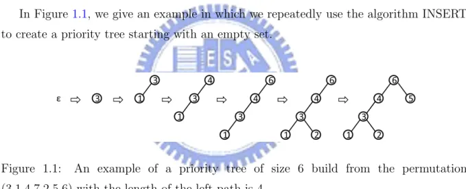
In Figure 1.1, we give an example in which we repeatedly use the algorithm INSERT to create a priority tree starting with an empty set.

Figure 1.1: An example of a priority tree of size 6 build from the permutation (3,1,4,7,2,5,6) with the length of the left path is 4.

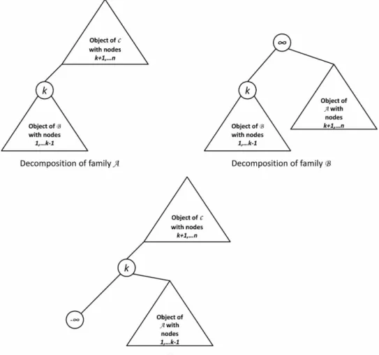
Deleting an element with the highest priority and inserting a new element are the main operations on priority trees. Hence, it is important to thoroughly analyze the running time of these operations. Therefore, we will use a random model on the input. More precisely, we consider the model where all n! permutations of the numbers 1, . . . , n generating all the p-trees of size n are equally likely. Then, characteristic parameters describing the running time become random variables. Apart from the model proposed above (called A in the sequel) we will need two more models: the model obtained by generating a priority

tree from a random permutation starting with positive infinity ”+∞” (this model will be called B) and the model obtained by generating a priority tree from a random permutation starting with negative infinity ”−∞” (this model will be called C). Moreover, we make the convention that both +∞ and −∞ do not count towards the size of the p-tree. The reason for considering these three models lies in the natural decomposition obtained by conditioning on the first element in the random permutation (where again +∞ and −∞ do not count); see Figure 1.2. The idea for this decomposition is not new and seems to have appeared first in a paper of A. Panholzer and H. Prodinger [12].

1.2.2

Previous results on priority trees

Length of the left path

In [12], A. Panholzer and H. Prodinger investigated the length of the left path in a p-tree of size n, where the length is by definition the number of nodes (for the model C we make the convention that −∞ does not count). This parameter describes the cost of the running time of the algorithm DELETE from the previous section. Under the random model above, the authors obtained mean and variance and proved a central limit theorem. We briefly sketch their method of proof.

1. Let An,m, Bn,m, and Cn,m be the probabilities that a random tree of A, B, and C with size n has a left path of length m. Then, by the decomposition from Figure

1.2, we have the following recurrences:

An,m = 1 n n X k=1 m X i=0 Cn−k,iBk−1,m−i ∀n ≥ 1, Bn,m = 1 n n X k=1 Bk−1,m−1 ∀n ≥ 1, Cn,m = 1 n n X k=1 Cn−k,m−1 ∀n ≥ 1. (1.9)

Consider the bivariate generating functions

A(z, v) = X n≥0 X m≥0 An,mznvm, B(z, v) = X n≥0 X m≥0 Bn,mznvm, C(z, v) =X n≥0 X m≥0 Cn,mznvm.

From (1.9), we have the following system of differential equations: ∂ ∂zA(z, v) = B(z, v)C(z, v), ∂ ∂zB(z, v) = v 1 − zB(z, v), ∂ ∂zC(z, v) = v 1 − zC(z, v). (1.10)

This system is easily solved and we obtain B(z, v) = v (1 − z)v, C(z, v) = 1 (1 − z)v, and ∂ ∂zA(z, v) = v (1 − z)2v A(z, v) = 1 1 − 2v µ 1 − v − v (1 − z)2v−1 ¶ . (1.11)

2. Now, denoted by An, Bn, and Cn the expectations of the length of the left paths in objects of size n in the families A, B resp. C. Moreover, define A(z) := ∂

∂vA(z, v) ¯ ¯ v=1, B(z) := ∂ ∂vB(z, v) ¯ ¯ v=1, and C(z) := ∂ ∂vC(z, v) ¯ ¯

v=1which are the ordinary generating functions of An, Bn, and Cn. By differentiating and reading of the coefficients of

A(z), B(z), and C(z) in (1.11), we have

An = 2Hn− 1 ∀n ≥ 1, A0 = 0,

Bn = Hn+ 1 ∀n ≥ 1, B0 = 0,

Cn = Hn ∀n ≥ 1, C0 = 0.

3. Differentiating equation (1.11) twice with respect to v and evaluating at v = 1 yields second factorial moments . For instance the second factorial moment ˇAn of the length of the left path in a p-trees of size n from random model A is given by

ˇ

An= 4Hn2− 4Hn− 4Hn(n)+ 4 ∀n ≥ 1 Aˇ0 = 0.

Consequently, the variance ˆAn is given by ˆ

An = ˇAn+ An− A2n = 2 log n + O (1) .

4. Let An(v) = _n1[zn]_∂z∂A(z, v). From (1.11) and singularity analysis (see Chapter VI in P. Flajolet and R. Sedgewick [5]), we obtain

An(v) = 1 n £ zn−1¤ ∂ ∂zA(z, v) = 1 n £ zn−1¤ ∂ ∂z v (1 − z)2v = v 2v − 1 µ n + 2v − 2 n ¶ = vn 2v−2 Γ(2v) µ 1 + O µ 1 n ¶¶ . (1.12)

for fixed v and n → ∞. Next, let

ϕΩ∗(t) = e−iµnt/σnA_n ¡ eit/σn¢_. By (1.12), we have An ¡

eit/σn¢_{= exp}¡_2(eit/σn_{− 1) log n}¢_{(1 + o(1))}

= exp µ 2 log nit σn −t 2 2 ¶ (1 + o(1)) . Then, as n → ∞, ϕΩ∗(t) = exp µ −2 log nit σn ¶ exp µ 2 log nit σn − t2 2 ¶ (1 + o(1)) = e−t2_/2 (1 + o(1)) → e−t2_/2 .

By L´evy’s continuity theorem, the central limit theorem follows from this.

We will provide another proof of the above result by using the method of moments. In doing so, we will encounter similar problems as in Example 2 in Section 1. However, we will overcome these problems by introducing some new ideas (for more details see the next example below). It should be mentioned here that from a technical point of view our proof is more complicated then the above one. So, this example will be mainly used to introduce our new approach.

The number of key comparisons when inserting a random element:

M. Kuba and A. Panholzer [9] considered the number of key comparisons when inserting a random element in a p-tree. This parameter describes the running time of the algorithm

INSERT. They authors sketched a proof of a limit law of this quantity (mean and variance were already discussed earlier in [12]). We will repeat their arguments here.

1. Let A[I]n , Bn[I], and Cn[I] be the random variables that count the number of key comparisons when inserting a randomly chosen element from {j + 1

2 : 0 ≤ j ≤ n}

into a random p-tree of the families A, B, and C with size n. Let

A(z, v) :=X n≥1 X m>0 nP¡A[I] n = m ¢ zn_vm_,

and similar we define B(z, v) and C(z, v). Then, by the decomposition from Section 1.2.1, we have the following system of differential equations:

∂ ∂zA(z, v) = 1 1 − zC(z, v) + 1 (1 − z)evB(z, v), ∂ ∂zB(z, v) = e2v 1 − zA(z, v) + ev 1 − zB(z, v), ∂ ∂zC(z, v) = 1 1 − zC(z, v) + e2v (1 − z)evA(z, v),

with initial conditions A(0, v) = 1, and B(0, v) = C(0, v) = ev_.

By solving for A(z, v) we get the following homogeneous third order linear differential equation for A(z, v):

∂ ∂z3A(z, v) − 3 + 2v 1 − z ∂2 ∂z2A(z, v) + 2v µ 2 (1 − z)2 − v (1 − z)v+1 ¶ ∂ ∂zA(z, v) + 2v2 (1 − z)v+2A(z, v) = 0, with initial conditions A(0, v) = 0, ∂

∂zA(z, v) ¯ ¯ z=0= v, ∂2 ∂z2A(z, v) ¯ ¯ ¯ z=0= 2v(v + 1). 2. Let Hr(z) := ∂ r

∂vrH(z, v), where H(z, v) = _∂z∂ ((1 − z)A(z, v)). Then from the above

equation we get the following differential equation:

H00 r(z) − 2 1 − zH 0 r(z) − 2 (1 − z)2Hr(z) = Sr(z),

where Sr(z) is the inhomogeneous part. Using variation of parameters then yields the following solution

Hr(z) = 1 3(1 − z)2 Z _z 0 (1 − t)3_S r(t)dt − 1 − z 3 Z _z 0 Sr(t)dt + Cr,1 (1 − z)2 + Cr,2(1 − z), (1.13) where Cr,1 and Cr,2 are suitable constants.

3. By using induction, Hr(z) is shown to exhibit the form Hr(z) = 2r X m=0 α(m) r 1 (1 − z)2L(z) 2r−m₊ 2r−2_X m=0 β(m) r (1 − z)L(z)2r−2−m, (1.14) where α(m)r and βr(m) are some constants which satisfy some recurrences and L(z) := log( 1 1−z). 4. Let Ar(z) := ∂ r ∂vrA(z, v) ¯ ¯ v=1 = P n≥1nE ³³ A[I]n ´_r´ zn_{, where E}³³_A[I] n ´_r´ denote the r−th factorial moment. By equation (1.14), Ar(z) satisfies the same type of expansion as Hr(z). Therefore by reading of the coefficients of _(1−z)1 2L(z)2r−m, we

obtain E³¡A[I] n ¢r´ = 2r X m=0 (log n)2r−m m X j=0 cr,j µ 2r − j m − j ¶ + O µ 1 n1−² ¶ , where cr,n are some constants and ² is a small constant.

5. Finally, the central moments are obtained from E µµ A[I]_n −1 3log 2_n ¶_r¶ = r X k=0 µ r k ¶ (−1)r−k µ 1 3 ¶_r−k

(log2r−2kn)E³¡A[I]_n ¢k ´ . and E³¡A[I] n ¢k´ = k X r=0 ½ k r ¾ E³¡A[I] n ¢r´ ,

by using the expansion from Step 4 (©k_rª denotes the Stirling numbers of first kind). The limits of the central moments are then computed via these exact expressions. The most complicated step in the proof of A. Panholzer and M. Kuba is the fifths one. This is due to the appearance of many cancellations in the central moments. Hence, the

authors needed a rather precise knowledge of the coefficients in the expansion from Step 4. This part can be simplified by shifting the mean as in the Examples from Section 1.1 and using induction. Then, we however encounter again the same problem as in Example 2 from Section 1.1. Therefore, we will first study the (non-central) moments. In order to do so, we will again use induction. Once the behavior of the non-central moments is clear, we will use this as input for the second induction. This will help us to overcome the problem observed in Section 1.1.

Overall, our method will turn out to be structurally easier than the one used by A. Panholzer and M. Kuba. Carrying out all details is, however, still rather messy. Therefore, as already mentioned before, we will introduce our method by analyzing first the length of the left path.

Chapter 2

Length of the Left Path

2.1

Statement of the result

As already mentioned in Chapter 1, in this chapter we will use the method of moments to give a second proof of the results on the length of the left path from Section 1.2.2. Even though this new proof will be much more complicated, this example is technically easier than the one considered in the next chapter. Hence, we will use this example as a kind of warm up in order to explain details concerning our new approach.

Now, let A[L]n , Bn[L] resp. Cn[L]be the length of the left path in a random size-n priority tree of the families A, B resp. C. Then, from the decomposition of Section 1.2.1, we obtain A[L] n d = B_I[L]_n−1+ C_n−I[L] _n ∀n ≥ 1, (2.1) B[L] n d = 1 + B_I[L]_n−1 ∀n ≥ 1, (2.2) C[L] n d = 1 + C_n−I[L] _n ∀n ≥ 1, (2.3)

where A[L]₀ = 0, B₀[L] = 1, C₀[L]= 0 and the distribution of In is given by P(In= j) =

1

n, for all 1 ≤ j ≤ n.

Theorem 2. The length of the left path A[L]n in a random size-n priority tree is asymp-totically Gaussian distributed:

A[L]n − E ³ A[L]n ´ r Var ³ A[L]n ´ −→ N(0, 1).d

Moreover, the mean value and variance satisfy E¡A[L] n ¢ ∼ 2 ln n, Var¡A[L] n ¢ ∼ 2 ln n.

2.2

Proof of the result - Theorem

2

The steps of this proof are similar to Example 1 in Chapter 1. In order to get all the central moments, first we need to find the mean values of A[L]n , Bn[L], and Cn[L]. Let

Pn(t) := E(eA [L] n t), Qn(t) := E(eBn[L]t), Tn(t) := E(eC [L] n t).

By the distributional recurrences form Section 2.1, we get Pn(t) = 1 n n X k=1 Qk−1(t)Tn−k(t) ∀n ≥ 1, (2.4) Qn(t) = 1 ne t n X k=1 Qk−1(t) ∀n ≥ 1, (2.5) Tn(t) = 1 ne t n X k=1 Tk−1(t) ∀n ≥ 1, (2.6)

with initial conditions P0(t) = 1, Q0(t) = et and T0(t) = 1.

Let Pn[r] = d r dtrPn(t) ¯ ¯ t=0, Q [r] n = d r dtrQn(t) ¯ ¯ t=0 and T [r] n = d r dtrTn(t) ¯ ¯ t=0. Hence, P[r] n = 1 n r X i=0 µ r i ¶_Xn k=1 Q[i]_k−1T_n−k[r−i] ∀n ≥ 1, (2.7)

Q[r]_n = 1 n n X k=1 Q[r]_k−1+ 1 n r X i=1 µ r i ¶_Xn k=1 Q[r−i]_k−1 ∀n ≥ 1, (2.8) T[r] n = 1 n n X k=1 T_k−1[r] + 1 n r X i=1 µ r i ¶_Xn k=1 T_k−1[r−i] ∀n ≥ 1, (2.9) with initial conditions P₀[i] = 0, Q[i]₀ = 1 and T₀[i] = 0 for all i ≥ 1 and P₀[0] = Q[0]₀ = T₀[0] = 1.

Note that by (2.8) and (2.9), all moments of B[L]n and Cn[L] satisfy a recurrence of the same type. Later on we will see that the same recurrence is satisfied by the central moments as well. Hence, we first study this recurrence in the next lemma.

Lemma 1. Consider the recurrence an= bn+_n1 P_n

k=1ak−1, where a0, {bn}n≥0 are given.

Then, for n ≥ 1, an = bn+ n X k=2 1 kbk−1+ a0. Proof. Because nan− (n − 1)an−1= nbn− (n − 1)bn−1+ an−1. Therefore an= bn− n − 1 n bn−1+ an−1, n ≥ 1 = bn+ n X k=2 1 kbk−1+ a0.

We use Lemma 1 to obtain asymptotic expansions of the mean values. Lemma 2. The mean values of A[L]n , Bn[L] and Cn[L] satisfy, as n → ∞,

E(A[L] n ) = 2 ln n + 2γ − 1 + O µ log n n ¶ , E(B[L] n ) = ln n + γ + 1 + O µ 1 n ¶ , E(C[L] n ) = ln n + γ + O µ 1 n ¶ .

Proof. Taking r = 1 in equation (2.7), (2.8) and (2.9), E(A[L] n ) = Pn0(0) = 1 n n X k=1 (E(B_k−1[L] ) + E(C_k−1[L] )) ∀n ≥ 1, (2.10) E(B[L] n ) = Q0n(0) = 1 + 1 n n X k=1 E(B_k−1[L] ) ∀n ≥ 1, (2.11) E(C_n[L]) = T_n0(0) = 1 + 1 n n X k=1 E(C_k−1[L] ) ∀n ≥ 1, (2.12)

where E(A[L]₀ ) = 0, E(B₀[L]) = 1 and E(C₀[L]) = 0. Hence, by Lemma 1, E(B[L] n ) = 1 + n X k=2 1 k + 1 = Hn+ 1 = ln n + γ + 1 + O µ 1 n ¶ ∀n ≥ 1, E(C[L] n ) = 1 + n X k=2 1 k = Hn = ln n + γ + O µ 1 n ¶ ∀n ≥ 1. From equation (2.10), we have

E(A[L] n ) = 1 n à n X k=1 E(B_k−1[L] ) + E(C_k−1[L] ) ! = 1 n à 1 + n X k=2 2 ln(k − 1) + 2γ + 1 + O µ 1 k − 1 ¶! . By Euler-Maclaurin summation formula,

E(A[L] n ) = 2 n µZ _n−1 1 ln x dx + ln(n − 1) 2 + c + O µ 1 n ¶¶ + 2γ + 1 + O µ log n n ¶ , where c is a constant. Then,

E(A[L] n ) = 2 ln n + 2γ − 1 + O µ log n n ¶ .

The next lemma extends the expansions from Lemma 2 to all higher moments. In particular, this lemma will be the crucial new tool for overcoming the problem we have countered in Step 3 of Example 2 of Chapter 1.

Let Pol_n(x) represent a polynomial in x with maximum degree ≤ n and Pol(x) rep-resent a polynomial in x without any restriction to the degree.

Lemma 3. The expansions of the r-th moments of A[L]n , Bn[L] and Cn[L] satisfy, as n → ∞ E¡A[L]_n ¢r = Pol(log n) + O µ 1 n1−² ¶ , E¡B_n[L]¢r = Pol(log n) + O µ 1 n1−² ¶ , E¡C_n[L]¢r = Pol(log n) + O µ 1 n1−² ¶ , where ² denotes an arbitrarily small constant ² > 0.

Proof. First, we will prove the result for E ³

Bn[L] ´_r

. We use induction on r. By Lemma

2, r = 1 is true. Now,we assume that the claim with exponents less than r is true. By equation (2.8), Q[r] n = 1 n n X k=1 Q[r]_k−1+ 1 n r X i=1 µ r i ¶_Xn k=1 Q[r−i]_k−1 | {z } :=bn .

By induction hypothesis, Q[r−i]_k = Pol(log k)+O¡ 1

k1−²

¢

for all i = 1, . . . , r, where ² denotes an arbitrarily small constant ² > 0. Therefore,

bn = 1 n à _r X i=1 µ n i ¶ Q[r−i]₀ + n−1 X k=1 Pol(log k) + O µ 1 k1−² ¶! = 1 n n−1 X k=1 Pol(log k) + 1 n n−1 X k=1 O µ 1 k1−² ¶ + O µ 1 n ¶ = Pol(log n) + O µ 1 n1−² ¶ . Then, we know Q[r] n = bn+ n X k=2 1 kbk−1+ 1 = Pol(log n) + O µ 1 n1−² ¶ + n X k=2 1 k µ Pol(log k − 1) + O µ 1 (k − 1)1−² ¶¶ = Pol(log n) + O µ 1 n1−² ¶ + n X k=2 O µ 1 k 1 (k − 1)1−² ¶

= Pol(log n) + O µ 1 n1−² ¶ + n X k=2 O µ 1 k 1 (k − 1)1−² ¶ = Pol(log n) + O µ 1 n1−² ¶ + ∞ X k=2 O µ 1 k 1 (k − 1)1−² ¶ | {z } =constant − ∞ X k=n+1 O µ 1 k 1 (k − 1)1−² ¶ = Pol(log n) + O µ 1 n1−² ¶ . The claims for E

³ A[L]n ´_r and E ³ Cn[L] ´_r

are proved similarly.

Now, we turn to central moments. Therefore, let Φn(t) := e−pnt_{Pn(t), Ψn(t) :=}

e−qntQ

n(t) and Ωn(t) := e−tntTn(t) where pn = E(A[L]n ), qn = E(Bn[L]) and tn = E(Cn[L]), Let Φ[r]n = Φ(r)n (0),Ψ[r]n = Ψn(r)(0) and Ω[r]n = Ω(r)n (0). Then by equation (2.4), (2.5) and (2.6), we have Φ[r] n = 1 n X i1+i2+i3=r n X k=1 µ r i1, i2, i3 ¶ Ψ[i1] k−1Ω [i2] n−k(∆Φn,k)i3 ∀n ≥ 1, (2.13) Ψ[r] n = 1 n n X k=1 Ψ[r]_k−1+ 1 n n X k=1 r−1 X i=0 µ r i ¶ Ψ[r]_k−1(∆Ψ n,k)r−i ∀n ≥ 1, (2.14) Ω[r] n = 1 n n X k=1 Ω[r]_k−1+ 1 n n X k=1 r−1 X i=0 µ r i ¶ Ω[r]_k−1(∆Ω n,k)r−i ∀n ≥ 1, (2.15)

with initial conditions Φ[i]₀ = Ψ[i]₀ = Ω[i]₀ = 0, for all i ≥ 1 and Φ[0]₀ = Ψ[0]₀ = Ω[0]₀ = 1, where ∆Φ

n,k = qk−1+ tn−k − pn, ∆Ψn,k = 1 − qn+ qk−1 and ∆Ωn,k = 1 − tn+ tk−1. First we consider the variance.

Lemma 4. The variances of A[L]n , Bn[L] and Cn[L] satisfy, as n → ∞,

Var(A[L]_n ) ∼ 2 log n, Var(B[L]_n ) ∼ log n, and Var(C_n[L]) ∼ log n.

Proof. First, we consider Var(Bn[L]). Since Ψ[1]n = 0 and by equation (2.14), we obtain

Var(B[L] n ) = Ψ[2]n = 1 n n X k=1 Ψ[2]_k−1+ 1 n n X k=1 (∆Ψ n,k)2 | {z } bn:= .

Next, we have bn= 1 n n X k=1 (∆Ψ_n,k)2 = 1 n n X k=1 (1 − qn+ qk−1)2 ∼ 1 n n X k=2 (1 − log n + log(k − 1))2 ∼ Z ₁ 0 (1 + log x)2dx ∼ 1. Hence by Lemma 1, Var(B[L] n ) ∼ 1 + n X k=1 1 k ∼ log n. Similarly, Var(C[L] n ) ∼ log n.

By the relation between Φ[2]n , Ψ[2]n ∼ log n, and Ω[2]n ∼ log n, we have Var(A[L]_n ) = Φ[2]_n = 1 n à n X k=1 Ψ[2]_k−1+ n X k=1 Ω[2]_n−k+1+ n X k=1 (∆Φ n,k)2 ! ∼ 1 n à _n X k=2 2 log(k − 1) + n X k=1 (qk−1+ tn−k+1− pn)2 ! ∼ 1 n à _n X k=2 2 log(k − 1) + n X k=2

(log(k − 1) + log(n − k + 1) − 2 log n)2 !

∼ 2 log n.

So far, we have treated means, variances, and all moments. So what is left is to consider

r-th central moments with r ≥ 1. From equation (2.13), the r-th central moment of A[L]n

is a combination of the central moments of Bn[L] and Cn[L]. Therefore, we first consider central moments of the latter two random variables.

Lemma 5. The r-th centralized and normalized moments of Bnand Cnsatisfy, as n → ∞, E ÃÃ Bn[L]− log n √ log n !_r! = ( (2m)! 2m_m!+ o (1) , if r = 2m, o (1) , if r = 2m + 1. (2.16) E ÃÃ Cn[L]− log n √ log n !_r! = ( _(2m)! 2m_m!+ o (1) , if r = 2m, o (1) , if r = 2m + 1. (2.17)

Proof. First, we consider Ψ[r]n . We use induction on r. By Lemma 2 and Lemma 4, we

know that the claim holds for r = 1 and r = 2. Now, we assume that the claim with exponents less than r is true. We consider the two cases r is even and r is odd in equation (2.14). Case 1: If r = 2m, then Ψ[2m] n = 1 n n X k=1 Ψ[2m]_k−1 + 1 n n X k=1 2m−1_X i=0 µ 2m i ¶ Ψ[i]_k−1(∆Ψ n,k)2m−i | {z } bn:= , where ∆n,k = 1 − qn+ qk−1.

We consider two parts according to whether i is even or not,

bn= 1 n m−1_X i=0 n X k=1 µ 2m 2i ¶ Ψ[2i]_k−1(∆Ψ n,k)2(m−i) | {z } αn:= + 1 n m X i=1 n X k=1 µ 2m 2i − 1 ¶ Ψ[2i−1]_k−1 (∆Ψ_n,k)2(m−i)+1 | {z } βn:= .

First, we consider αn and use the induction hypothesis to get the following :

αn= 1 n m−1_X i=0 n X k=1 µ 2m 2i ¶ Ψ[2i]_k−1(∆Ψ_n,k)2(m−i) ∼ m−1_X i=1 µ 2m 2i ¶ (2i)! 2i_i! 1 n n X k=2

logi(k − 1)(1 − log(n) + log(k − 1))2(m−i)

| {z }

:=Ti

Now, we just consider Ti for 1 ≤ i ≤ m − 1. By integral approximation, Ti = 1 n n X k=2 µ log n + log µ k − 1 n ¶¶_i

(1 − log(n) + log(k − 1))2(m−i)

∼ login

Z ₁

0

(1 + log x)2(m−i)dx

∼ cilogin,

where ci is a constant. Hence, we know that i = m − 1 gives the main contribution of αn. Consequently, αn∼ 1 n n−1 X k=1 µ 2m 2m − 2 ¶ (2m − 2)! 2m−1_{(m − 1)!}log m−1_{(k)(1 − log(n) + log(k))}2 ∼ µ 2m 2m − 2 ¶ (2m − 2)! 2m−1_{(m − 1)!}log m−1_{n =} (2m)! 2m_{(m − 1)!}log m−1_n. (2.18) Now, we consider βn, βn= 1 n m X i=1 n X k=1 µ 2m 2i − 1 ¶ Ψ[2i−1]_k−1 (∆Ψ n,k)2(m−i)+1. Similarly as above, for i ≤ m − 1 we obtain the bound o

³

logm−32 n

´

. So what is left is to look at the contribution of i = m which is

T := 1 n n X k=1 2mΨ[2m−1]_k−1 ∆Ψ n,k.

By Lemma 3, Ψ[2m−1]_k−1 is a polynomial in log n. Therefore by induction hypothesis, we know that Ψ[2m−1]_k−1 ∼ Pm−1_i=0 cilogi(k − 1), where the ci’s are suitable constants for all i. Consequently, T ∼ 2m n n X k=2 Ã m−1_X i=0 cilogi(k − 1) ! ∆Ψ n,k = 2m n n X k=2 Ã m−1_X i=0 cilogi(k − 1) ! (1 − log(n) + log(k − 1)). Using integral approximation,

T ∼ c logm−1n Z ₁ 0 (1 + log x) dx | {z } =0 ⇒ T = o¡logm−1n¢. (2.19) Overall, βn= o ¡

logm−1n¢. Next, by equation (2.18) and (2.19),

bn = αn+ βn ∼ (2m)! 2m_{(m − 1)!}log m−1_n. By Lemma 1, Ψ[2m]_n = bn+ n X k=2 1 kbk−1 ∼ (2m)! 2m_m! log m_n. Therefore, E   Ã Bn[L]− log n √ log n !_2m  = (2m)! 2m_m! + o(1), as n → ∞. Case 2: If r = 2m + 1, then Ψ[2m+1] n = 1 n n X k=1 Ψ[2m+1]_k−1 + 1 n n X k=1 2m X i=0 µ 2m + 1 i ¶ Ψ[i]_k−1(∆Ψ n,k)2m+1−i | {z } bn:= ,

where ∆n,k = 1 − qn+ qk−1. We consider again two parts according to whether i is even or not: bn = 1 n m X i=0 n X k=1 µ 2m + 1 2i ¶ Ψ[2i]_k−1(∆Ψ_n,k)2m+1−2i | {z } αn:= + 1 n m X i=1 n X k=1 µ 2m + 1 2i − 1 ¶ Ψ[2i−1]_k−1 (∆Ψ n,k)2(m−i)+2 | {z } βn:= .

First, we will treat αn. Similarly as in Case 1, we only have to consider the term i = m. Hence by using the induction hypothesis, we have

αn∼ 1 n n X k=2 µ 2m + 1 2m ¶ (2m)! 2m_m! log m_{(k − 1) (1 − log n + log(k − 1)) .}

Again by integral approximation, we have αn∼ µ 2m + 1 2m ¶ (2m)! 2m_m! log m_n Z ₁ 0 (1 − log x)dx = o (logmn) .

For βn, we can argue similarly:

βn∼ 1 n n X k=1 µ 2m + 1 2m − 1 ¶ Ψ[2m−1]_k−1 (∆Ψ n,k)2. By using induction hypothesis, we have

βn = 1 n n X k=2 µ 2m + 1 2m − 1 ¶ o ³ logm−12(k − 1) ´ (∆Ψ n,k)2 = o ³ logm−12 n ´ . Therefore, we know bn= αn+ βn = o ³ logm−1_{2 n}´_. By Lemma 1, Ψ[2m+1] n = o ³ logm−12 n ´ + n X k=2 1 ko ³ logm−12(k − 1) ´ = o³logm+1_{2 n}´_. Hence, as n → ∞, E   Ã Bn[L]− log n √ log n !_2m+1  = o (1) . Similarly, as n → ∞, E ÃÃ Cn[L]_√− log n log n !_r! = ( (2m)! 2m_m! + o (1) , if r = 2m, o (1) , if r = 2m + 1.

Lemma 6. The r-th centralized and normalized moment of A[L]n satisfies, as n → ∞, E ÃÃ A[L]n − 2 log n √ 2 log n !_r! = ( (2m)! 2m_m!+ o (1) , if r = 2m, o (1) , if r = 2m + 1. (2.20)

Case 1: If r = 2m, then Φ[2m] n = 1 n X i1+i2+i3=2m n X k=1 µ 2m i1, i2, i3 ¶ Ψ[i1] k−1Ω [i2] n−k(∆Φn,k)i3, where ∆n,k = qk−1+ tn−k− pn.

Then, we consider three parts according to whether i1, i2 ∈ odd, i3 = 0 or i1, i2 ∈ even,

i3 = 0 or i3 6= 0. Φ[2m] n = 1 n X i1+i2=m n X k=1 µ 2m 2i1 ¶ Ψ[2i1] k−1Ω [2i2] n−k | {z } αn:= + 1 n X i1+i2=m−1 n X k=1 µ 2m 2i1+ 1 ¶ Ψ[2i1+1] k−1 Ω [2i2+1] n−k | {z } βn:= + 1 n X i1+i2+i3=2m i36=0 n X k=1 µ 2m i1, i2, i3 ¶ Ψ[i1] k−1Ω [i2] n−k(∆Φn,k)i3 | {z } γn:= . First, we consider αn αn= 1 n X i1+i2=m n X k=1 µ 2m 2i1 ¶ Ψ[2i1] k−1Ω [2i2] n−k. By Lemma 5, we have αn ∼ 1 n X i1+i2=m n X k=1 µ 2m 2i1 ¶ µ (2i1)! 2i1i 1! logi1_{(k − 1)} ¶ µ (2i2)! 2i2i 2! logi2_{(n − k)} ¶ . Then, we have αn∼ X i1+i2=m µ 2m 2i1 ¶ (2i1)! 2i 1i1! (2i2)! 2i 2i2! logm_n = m X i=0 (2m)! (2m − 2i)!(2i)! (2i)! 2i_i! (2m − 2i)! 2m−i_{(m − i)!}log

m_n = (2m)! 2m log m_n m X i=0 1 i!(m − i)!

= (2m)! 2m log m_n2m m! = (2m)! 2m_m!2 m_logm_n.

Now, we consider βn and γn,

βn= 1 n X i1+i2=m−1 n X k=1 µ 2m 2i1+ 1 ¶ Ψ[2i1+1] k−1 Ω [2i2+1] n−k = 1 n X i1+i2=m−1 n−1 X k=2 µ 2m 2i1+ 1 ¶ o ³ logi1+1/2_{(k − 1) log}i2+1/2_{(n − k)} ´ = o (logmn)

For γn, i1+ i2 = 2m − 1 gives the main contribution. Consequently,

γn = 1 n X i1+i2+i3=2m i36=0 n X k=1 µ 2m i1, i2, i3 ¶ Ψ[i1] k−1Ω [i2] n−k(∆Φn,k)i3 = 1 n X i1+i2+i3=2m i36=0 n−1 X k=2 µ 2m i1, i2, i3 ¶ O ³ logi1/2_{(k − 1) log}i2/2_{(n − k)} ´ (∆Φ n,k)i3 = O ³ logm−12 n ´ . Therefore, Φ[2m] n = αn+ βn+ γn∼ (2m)! 2m_m!2 m_logm_n. Hence, E   Ã A[L]n − 2 log n √ 2 log n !_2m  = (2m)! 2m_m! + o(1). Case 2: If r = 2m + 1, Φ[2m+1]_n = 1 n X i1+i2+i3=2m+1 n X k=1 µ 2m + 1 i1, i2, i3 ¶ Ψ[i1] k−1Ω [i2] n−k(∆Φn,k)i3,

where ∆n,k = qk−1+ tn−k − pn. Now, we consider two parts according to whether i3 = 0

Φ[2m+1]_n = 1 n X i1+i2=2m+1 n X k=1 µ 2m + 1 i1 ¶ Ψ[i1] k−1Ω [i2] n−k | {z } αn:= + 1 n X i1+i2+i3=2m+1 i36=0 n X k=1 µ 2m + 1 i1, i2, i3 ¶ Ψ[i1] k−1Ω [i2] n−k(∆Φn,k)i3 | {z } βn:= .

First let us consider αn. By Lemma 5 we have the following equation:

αn ∼ 1 n X i1+i2=2m+1 n−1 X k=2 µ 2m + 1 i1 ¶ o ³ logi1/2_{(k − 1) log}i2/2_{(n − k)} ´ = o ³ logm+12(n) ´ .

For βn, the main contribution is given by i1+ i2 = 2m. Consequently,

βn = 1 n X i1+i2+i3=2m+1 i36=0 n X k=1 µ 2m + 1 i1, i2, i3 ¶ Ψ[i1] k−1Ω [i2] n−k(∆Φn,k)i3 = 1 n X i1+i2+i3=2m+1 i36=0 n X k=1 µ 2m + 1 i1, i2, i3 ¶ O³logi1/2_{(k − 1) log}i2/2_{(n − k)} ´ (∆Φ n,k)i3 = O (logmn) . Therefore, Φ[2m+1] n = αn+ βn= o ³ logm+1_2(n)´_. Then, E   Ã A[L]n − 2 log n √ 2 log n !_2m+1  = o(1) as n → ∞. By equation (1.1), this concludes the proof.

The proof of Theorem2now follows from the last proposition together with Theorem

Chapter 3

Number of key comparisons when

inserting a random node

3.1

Statement of the result

We will use once more the approach introduced in the last chapter to re-derive the result on the number of key comparisons when inserting a random node from Section 1.2.2. As explained before, our proof will be structurally easier than the previous proof.

Now, let A[I]n , Bn[I] and Cn[I] be the random variables that count the number of key comparisons when inserting a randomly chosen element p in {j + 1

2 : 0 ≤ j ≤ n} into a

random size-n tree of the families A, B and C. Moreover, let I be the first element in the random permutation (where +∞ and −∞ do not count in model B and C, respectively) and denote by ˜A (or ˜B or ˜C) the tree under consideration. Finally, let ˜B and ˜C (or ˜A and ˜C or ˜A and ˜B) be the trees in the decomposition from Section 1.2.1. Then, we have the following distributional recurrences,

A[I] n d = ( C_n−k[I] , if I = k and p ∈ ˜C, B_k−1[I] + L(c)_n−k, if I = k and p ∈ ˜B. B[I] n d = ( A[I]_n−k+ 2, if I = k and p ∈ ˜A, B_k−1[I] + 1, if I = k and p ∈ ˜B. (3.1)

C[I] n d = ( C_n−k[I] , if I = k and p ∈ ˜C, A[I]_k−1+ L(c)_n−k+ 2, if I = k and p ∈ ˜A,

with initial conditions A[I]₀ = 0, B₀[I] = C₀[I] = 1, where L(c)n = left path of ˜C and the distribution of In is given by

P (I = j) = 1

n, for all 1 ≤ j ≤ n. We will again use this to prove the following result.

Theorem 3. The number of key comparison, A[I]n , in a random size-n priority tree is asymptotically Gaussian distributed:

A[I]n − E ³ A[I]n ´ r Var ³ A[I]n ´ −→ N(0, 1).d

Moreover, the mean value and variance satisfy E¡A[I] n ¢ ∼ 1 3log 2_{n, Var}¡_A[I] n ¢ ∼ 10 81log 3_n.

3.2

Proof of the result - Theorem

3

By the distributional recurrences from Section 3.1, we get E ³ eA[I]n v ´ = n X k=1 E ³ eCn−k[I] v´ 1 n n − k + 1 n + 1 + n X k=1 E ³ eBk−1[I] v ´ E ³ eL(c)n−kv´ 1 n k n + 1 ∀n ≥ 1, (3.2) E ³ eB[I]n v ´ = n X k=1 e2vE ³ eA[I]n−kv´ 1 n n − k + 1 n + 1 + n X k=1 evE ³ eB[I]k−1v´ 1 n k n + 1 ∀n ≥ 1, (3.3) E ³ eCn[I]v ´ = n X k=1 E ³ eC_n−k[I] v´ 1 n n − k + 1 n + 1 + n X k=1 e2v_E³_eA[I]_k−1v´_E³_eL(c)_n−kv´ 1 n k n + 1 ∀n ≥ 1, (3.4)

with initial conditions E ³ eA[I]0 v ´ = 1, E ³ eB[I]0 v ´ = E ³ eC[I]0 v ´ = ev _{and E}³_eL(c)0 ´ = 1. Let A(z, v), B(z, v) and C(z, v) be the generating functions of A[I]n , Bn[I] and Cn[I],

A(z, v) := X n≥0 (n + 1)E ³ eA[I]n v ´ zn, B(z, v) := X n≥0 (n + 1)E ³ eB[I]n v ´ zn_, C(z, v) :=X n≥0 (n + 1)E ³ eCn[I]v ´ zn_.

By (3.2), (3.3) and (3.4), we get the following system of linear differential equations: ∂ ∂zA(z, v) = 1 1 − zC(z, v) + 1 (1 − z)evB(z, v), ∂ ∂zB(z, v) = e2v 1 − zA(z, v) + ev 1 − zB(z, v), ∂ ∂zC(z, v) = 1 1 − zC(z, v) + e2v (1 − z)evA(z, v),

with initial conditions A(0, v) = 1, and B(0, v) = C(0, v) = ev_.

This yields the following homogeneous third order linear differential equation for A(z, v),

∂3 ∂z3A(z, v) − 3 + 2ev 1 − z ∂2 ∂z2A(z, v) + 2e v µ 2 (1 − z)2 − ev (1 − z)ev₊₁ ¶ ∂ ∂zA(z, v) + 2e2v (1 − z)ev₊₂A(z, v) = 0, (3.5) with initial conditions A(0, v) = 1, ∂

∂z A(z, v)|z=0= 2ev, ∂

2

∂z2 A(z, v)|_z=0 = 2ev + 4e2v.

Our goal is to investigate E ³ eA[I]nt ´ . Hence let an(v) := [zn]A(z, v) = [zn]X n≥0 (n + 1)E ³ eA[I]n v ´ zn= (n + 1)E ³ eA[I]n v ´ . We can rewrite equation (3.5) to

∂3 ∂z3A(z, v) = 3 + 2ev 1 − z ∂2 ∂z2A(z, v) − 2e v 2 (1 − z)2 ∂ ∂zA(z, v) + ∂3 ∂z3g(z, v), (3.6)

where ∂3 ∂z3g(z, v) := 2e 2v (1−z)ev +1_∂z∂A(z, v) − 2e 2v (1−z)ev +2A(z, v).

Because equation (3.6) is a Cauchy Euler differential equations, by [3] we have the recur-rence, an(v) = n−1 X k=0 2 X j=1 cj(v) j! 3! ¡_k j ¢¡_n−1−k 2−j ¢ ¡_n 3 ¢ ak(v) + bn, (3.7)

where c1(v) = −4ev, c2(v) = 3 + 2ev and bn:= [zn]g(z, v). Hence,

an(v) = n−1 X k=0 à 2 X j=1 cj(v) j! 3! ¡_k j ¢¡_n−1−k 2−j ¢ ¡_n 3 ¢ +2e 2v 3! ¡¡_ev_+n−k−2 n−k−2 ¢ k −¡ev_n−k−3+n−k−2¢¢ ¡_n 3 ¢ ! ak(v). (3.8)

Next, we will prove that r-th moments are polynomial in log n. Therefore, we need to differentiate equation (3.8) r times with respect to v. In order to do so, we first proof the following lemma. Lemma 7. We have, dm dtm µ et_{+ n} n − 1 ¶¯_¯ ¯ ¯ t=0 = (n + 1)n 2 µ logm_{n + Pol} m−1(log n) + O µ 1 n1−² ¶¶ , (3.9) and dm dtm µ et_{+ n} n ¶¯_¯ ¯ ¯ t=0 = (n + 1) µ

logmn + Pol_m−1(log n) + O

µ 1

n1−²

¶¶

. (3.10)

Hence, we also have

dm dtme 2t µ et_{+ n} n − 1 ¶¯_¯ ¯ ¯ t=0 = (n + 1)n 2 µ logm_{n + Pol} m−1(log n) + O µ 1 n1−² ¶¶ , and dm dtme 2t µ et_{+ n} n ¶¯_¯ ¯ ¯ t=0 = (n + 1) µ logm_{n + Pol} m−1(log n) + O µ 1 n1−² ¶¶ .

Proof. First consider equation (3.9). We use induction on m. For, m = 1, we have

d dt µ et_{+ n} n − 1 ¶¯_¯ ¯ ¯ t=0 = d dt (et_{+ n)(e}t_{+ n − 1) · · · (e}t_{+ 2)} (n − 1)! ¯ ¯ ¯ ¯ t=0

= (e t_{+ n)(e}t_{+ n − 1) · · · (e}t_{+ 2)} (n − 1)! n X i=2 et et_{+ i} ¯ ¯ ¯ ¯ ¯ t=0 = (n + 1)n 2 n X i=2 1 1 + i = (n + 1)n 2 µ

log n + Pol₀(log n) + O µ

1 n

¶¶ .

Therefore, m = 1 is true. Now, we assume that the claim with exponent less than m is true. dm dtm µ et_{+ n} n − 1 ¶¯_¯ ¯ ¯ t=0 = d m dtm (et_{+ n)(e}t_{+ n − 1) · · · (e}t_{+ 2)} (n − 1)! ¯ ¯ ¯ ¯ t=0 = d m−1 dtm−1 (et_{+ n)(e}t_{+ n − 1) · · · (e}t_{+ 2)} (n − 1)! n X i=2 et et_{+ i} ¯ ¯ ¯ ¯ ¯ t=0 = m−1 X j=0 µ m − 1 j ¶ µ (et_{+ n)(e}t_{+ n − 1) · · · (e}t_{+ 2)} (n − 1)! ¶_(j) à _n X i=2 et et_{+ i} !_(m−1−j)¯_¯ ¯ ¯ ¯ ¯ t=0 = (n + 1)n 2 à _n X i=2 et et_{+ i} !_m−1 + m−1 X j=1 µ m − 1 j ¶ µ et_{+ n} n − 1 ¶_(j)Ã_Xn i=2 et et_{+ i} !_(m−1−j)¯_¯ ¯ ¯ ¯ ¯ t=0 | {z } :=Tj .

By the induction hypothesis, µ et_{+ n} n − 1 ¶_(j)¯_¯ ¯ ¯ ¯ t=0 = (n + 1)n 2 µ logj_{n + Pol} j−1(log n) + O µ 1 n1−² ¶¶ , and we can use induction to get the following equation,

à n X i=2 et et_{+ i} !_(m−j)¯_¯ ¯ ¯ ¯ ¯ t=0

= log n + Pol₀(log n) + O µ

1 n

¶

Hence, we know Tm−1 gives the main distribution. Then dm dtm µ et_{+ n} n − 1 ¶¯_¯ ¯ ¯ t=0 = (n + 1)n 2 µ logm_{n + Pol} m−1(log n) + O µ 1 n1−² ¶¶ . Similarly, we can prove that

dm dtm µ et_{+ n} n ¶¯ ¯ ¯ ¯ t=0 = (n + 1) µ

logmn + Pol_m−1(log n) + O

µ 1

n1−²

¶¶ . We can use the binomial expansion to get the following equation,

dm dtme 2t µ et_{+ n} n − 1 ¶¯_¯ ¯ ¯ t=0 = m X i=0 µ m i ¶ 2m−i µ et_{+ n} n − 1 ¶_(i)¯_¯ ¯ ¯ ¯ t=0 = (n + 1)n 2 µ

logmn + Pol_m−1(log n) + O

µ 1

n1−²

¶¶ . Similarly, we can prove that

dm dtme 2t µ et_{+ n} n ¶¯_¯ ¯ ¯ t=0 = (n + 1) µ

logmn + Pol_m−1(log n) + O

µ 1 n1−² ¶¶ . Let a[r]n = _n+11 d r dtran(v) ¯ ¯

v=0. Differentiating equation (3.8) r times with respect to v and evaluating at v = 0 leads then to the following recurrence,

(n + 1)a[r] n = n−1 X k=0 à ₂ X j=0 πj j! 3! ¡_k j ¢¡_n−1−k 2−j ¢ ¡_n 3 ¢ ! (k + 1)a[r]_k + bn, (3.11) where π0 = −2, π1 = −2, π2 = 5, and bn = n−1 X k=0 r X i=1 µ r i ¶  2 X j=1 cj(v) j! 3! ¡_k j ¢¡_n−1−k 2−j ¢ ¡_n 3 ¢ +2e2v 3! ³¡_ev_+n−k−2 n−k−2 ¢ k −¡et_n−k−3+n−k−2¢´ ¡_n 3 ¢   (i)¯_¯ ¯ ¯ ¯ ¯ ¯ t=0 (k + 1)a[r−i]_k . Lemma 8. The mean value of A[I]n satisfies, as n → ∞,

E¡A[I] n ¢ = 1 3log 2_{n + Pol} 1(log n) + O µ 1 n1−² ¶ , where ² denotes an arbitrarily small constant ² > 0.

Proof. Let r = 1 in equation (3.11), (n + 1)a[1] n = n−1 X k=0 à ₂ X j=0 πj j! 3! ¡_k j ¢¡_n−1−k 2−j ¢ ¡_n 3 ¢ ! (k + 1)a[1]_k + bn, where bn= n−1 X k=0 à ₂ X j=1 cj(v) j! 3! ¡_k j ¢¡_n−1−k 2−j ¢ ¡_n 3 ¢ +2e 2v 3! ¡¡_ev_+n−k−2 n−k−2 ¢ k −¡ev_n−k−3+n−k−2¢¢ ¡_n 3 ¢ !(1)¯¯ ¯ ¯ ¯ ¯ v=0 (k + 1). Now, we divide bn into two parts,

bn = αn+ βn, where αn= n−1 X k=0 à ₂ X j=1 cj(v) j! 3! ¡_k j ¢¡_n−1−k 2−j ¢ ¡_n 3 ¢ !(1)¯¯ ¯ ¯ ¯ ¯ v=0 (k + 1), and βn = n−1 X k=0 à 2e2v 3! ¡¡_ev_+n−k−2 n−k−2 ¢ k −¡ev_n−k−3+n−k−2¢¢ ¡_n 3 ¢ !₍₁₎¯_¯ ¯ ¯ ¯ ¯ v=0 (k + 1). For αn, by Euler-Maclaurin summation formula,

αn= n µ c + O µ 1 n ¶¶ , where c is some constant.

For βn, by Lemma 7, βn= n−1 X k=0 2 3!¡n₃¢ µ k(n − k − 1) µ log(n − k − 2) + c1+ O µ 1 (n − k − 2)1−² ¶¶ −(n − k − 1)(n − k − 2) 2 µ log(n − k − 2) + c2 + O µ 1 (n − k − 2)1−² ¶¶¶ (k + 1). where c1, c2 are constants. By Euler-Maclaurin summation formula,

βn= n µ 1 12log 2_{n + Pol} 1(log n) + O µ 1 n1−² ¶¶ .