新的加權平均損失管制圖 - 政大學術集成
165
0
0
全文
(2) 謝辭 很快的,兩年的研究生生活已經到了尾聲,回想起這兩年,經歷了很多事也 學習到很多,讓我成長了不少,也要感謝許多人這一路上的幫助與支持。 首先要感謝的是我的指導老師. 楊素芬教授,謝謝老師這兩年辛苦的指導,. 讓我學習到很多統計品管上的知識,也幫助我順利完成我的碩士論文,老師嚴格 的教導,使我有了更加積極的做事態度,也讓我更加重視做事的品質與效率。 接著我要感謝我的口試委員,鄭惟孝教授、曾勝滄教授與黃榮臣教授;感謝 鄭惟孝教授在我完成論文期間給予的指導與建議,使的本論文更加的完善,也謝. 政 治 大 解到此論文還有哪些地方不足而需要改進的地方。 立. 謝曾勝滄教授與黃榮臣教授仔細的閱讀本論文並提出許多的意見與想法,讓我了. 碩士生兩年期間,特別要感謝我的同學,雨築、鈞遠和至芬,以及班上的其. ‧ 國. 學. 他同學,因為有你們的陪伴,不管是一起努力學習或一起玩樂的日子,都讓我的. ‧. 生活更加精彩,也因為互相學習鼓勵而讓我成長了不少。. y. Nat. 最後一定要感謝的則是我的家人,家人是我的支柱以及動力的來源,謝謝你. er. io. sit. 們的陪伴與支持,以後的日子我也會更加努力的。. 本研究承蒙行政院國家科學委員會,計畫編號 NSC98-2118-M-004-005-MY2. n. al. 補助,謹此致謝。. Ch. engchi. i n U. v. 歐家玲 謹致 中華民國一百年六月. I.
(3) ABSTRACT. In recent years, a few researchers had proposed different types of single charts that jointly monitor the process mean and the variation. In this project, we use the weighted average loss (WL) to construct WL control charts for monitoring the process mean and variance simultaneously while the target value may be different from the in-control mean. This statistic WL applied a weighted factor to adjust the weights of the loss due to the square of the deviation of the process mean from the target and the. 政 治 大 charts. We not only construct the fixed parameters (FP) WL chart but also the adaptive 立 variance change. So the WL charts are more effective than unadjusted loss function. WL charts which included variable sampling interval (VSI) WL chart, variable sample. ‧ 國. 學. size and sampling interval (VSSI) WL chart and variable parameters (VP) WL chart.. ‧. We calculate the average run length (ARL) for FP WL chart and using Markov chain. sit. y. Nat. approach to calculate the average time to signal (ATS) for adaptive WL charts to. io. er. measure the performance and compare each other. From the comparison, we find the adaptive WL charts are more effective than the FP WL chart. We also proposed the. al. n. v i n C an optimal adaptive WL charts using technique to minimize ATS h eoptimization ngchi U. 1. (ARL1). when the process was out-of-control. In addition, in order to detect the small shifts of the process mean and variance effectively, we construct the WL charts using the EWMA scheme. The proposed charts are based on only one statistic and are more effective than the X S chart. And the WL charts are easy to understand and apply than using two charts for detecting the mean and variance shifts simultaneously. Keywords: Statistical process control; Weighted average loss; Adaptive control chart; Markov chain; Optimization technique; EWMA scheme. II.
(4) TABLE OF CONTENTS. CHAPTER 1. INTRODUCTION..................................................................................1 CHAPTER 2. THE DISTRIBUTION OF THE WEIGHTED AVERAGE LOSS.........5 2.1 Taguchi Loss Function and Its Expectation and Estimator................................5 2.2 The Estimator of the Expectation of the Loss Function and Weighted Average Loss......................................................................................................5 2.3 The Approximated Distribution of Weighted Average Loss..............................6. 政 治 大 WL CHARTS.......................................................................................11 立. CHAPTER 3. DESIGN AND ATS1 ANALYSIS OF THE FP, VSI, VSSI AND VP. 3.1 Design of the FP WL Control Chart.................................................................11. ‧ 國. 學. 3.2 Design of the VP WL Control Chart................................................................12. ‧. 3.3 ATS1 Analysis and ATS1 Comparison among the FP, VSI, VSSI and VP WL. sit. y. Nat. Charts................................................................................................................17. io. er. CHAPTER 4. DESIGN AND DATA ANALYSIS OF THE OPTIMAL FP, VSI, VSSI AND VP WL CHARTS .............................................................27. al. n. v i n CWL 4.1 Design of the Optimal FP Chart...................................................27 h eControl ngchi U. 4.2 Design of the Optimal VSI WL Control Chart.................................................27 4.3 Design of the Optimal VSSI WL Control Chart..............................................28 4.4 Design of the Optimal VP WL Control Chart..................................................29 4.5 ATS1 Analysis and ATS1 Comparison among the Optimal FP, VSI, VSSI and VP WL Charts...................................................................................................30 4.6 Performance Comparison among the Max, WT-WL and One-Sided FP WL Charts...............................................................................................................59 CHAPTER 5. DESIGN AND DATA ANALYSIS OF THE FP AND VSI EWMA. III.
(5) WL CHARTS.......................................................................................64 5.1 Design of the FP EWMA WL Chart................................................................64 5.2 Design of the VSI EWMA WL Chart..............................................................67 5.3 ATS1 Analysis and ATS1 Comparison among the FP EWMA, VSI EWMA and FP WL Charts............................................................................................71 5.4 Performance Comparison of the EWMA-CCX, EWMA-CR and One-Sided FP EWMA WL Control Charts............................................................................119 CHAPTER 6. AN EXAMPLE...................................................................................125. 政 治 大 REFERENCES...........................................................................................................142 立 APPENDIX................................................................................................................145 CHAPTER 7. CONCLUSION AND FUTURE RESEARCH...................................140. ‧. ‧ 國. 學. n. er. io. sit. y. Nat. al. Ch. engchi. IV. i n U. v.
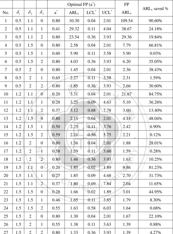
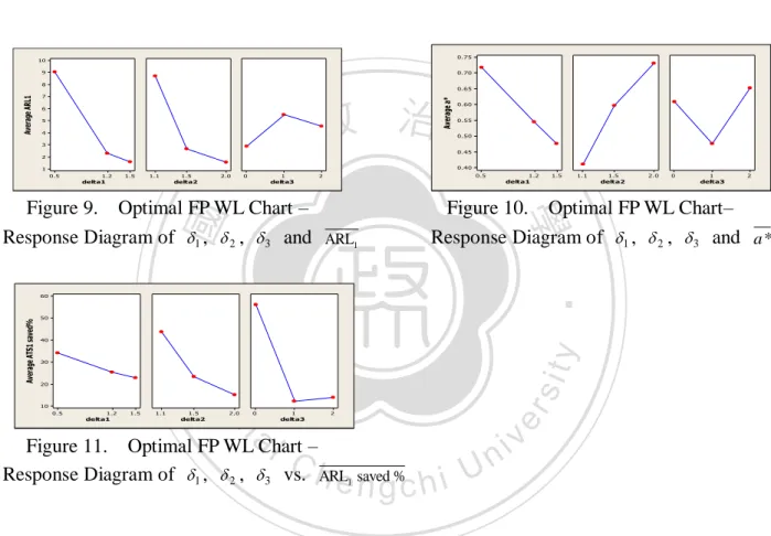
(6) LIST OF TABLES Table 1. Definition of Process States for the VP WL Chart.................................15. Table 2. ARL1 for FP WL Chart...........................................................................18. Table 3. FP WL Chart– Response Table of 1 , 2 , 3 and ARL1 ..................18. Table 4. ATS1 for VSI WL Chart and ATS1 saved % for VSI with FP WL Chart ................................................................................................................20. Table 5. VSI WL Chart– Response Table of 1 , 2 , 3 and ATS1 ................21. Table 6. ATS1 and ANOS for VSSI WL Chart and ATS1 saved % and ANOS. 政 治 大. Saved % for VSSI with FP WL Chart.....................................................22. 立. VSSI WL Chart –Response Table of 1 , 2 , 3 vs. ATS1 and. 學. ‧ 國. Table 7. ANOS .....................................................................................................23 ATS1 and ANOS for VP WL Chart and ATS1 saved % and ANOS Saved. ‧. Table 8. y. sit. VP WL Chart –Response Table of 1 , 2 , 3 vs. ATS1 and. io. n. al. er. Table 9. Nat. % for VP with FP WL Chart.................................................................25. i n U. v. ANOS .....................................................................................................26 Table 10. Ch. engchi. ARL1 for Optimal FP WL Chart and ARL1 saved % for Optimal FP with FP WL Chart.................................................................................31. Table 11. Optimal FP WL Chart –Response Table of 1 , 2 , 3 vs. ARL1 , 1 ,. 2 , 3 vs. a * and 1 , 2 , 3 vs. ARL1 saved % .........................32 Table 12. ATS1 for Optimal VSI WL Chart and ATS1 saved % for Optimal VSI with FP WL Chart when a = 0.6...........................................................34. Table 13. Optimal VSI WL Chart –Response Table of 1 , 2 , 3 vs. ATS1 and 1 , 2 , 3 vs. ATS1 saved % .....................................................35. V.
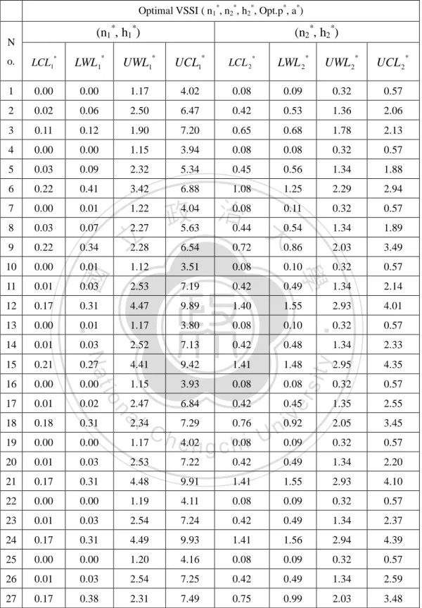
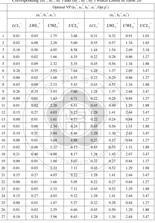
(7) Table 14. ATS1 for Optimal VSI WL Chart and ATS1 saved % for Optimal VSI with FP WL Chart when a is not Specified..........................................37. Table 15. Optimal VSI WL Chart –Response Table of 1 , 2 , 3 vs. ATS1 ,. 1 , 2 , 3 vs. a * and 1 , 2 , 3 vs. ATS1 saved % ...................38 Table 16. ATS1 and ANOS for Optimal VSSI WL Chart and ATS1 Saved % and ANOS Saved % for Optimal VSSI with FP WL Chart when a = 0.6...40. Table 17. The Control Limits and Warning Limits of the Optimal VSSI Chart with Corresponding (nq, hq), q = 1, 2 Listed in Table 18......................41. Table 18. 政 治 大. Optimal VSSI WL Chart –Response Table of 1 , 2 , 3 vs. ATS1. 立. and 1 , 2 , 3 vs. ATS1 saved % .....................................................42. ‧ 國. 學. Table 19. Optimal VSSI WL Chart –Response Table of 1 , 2 , 3 v.s.. ATS1 and ANOS for Optimal VSSI WL Chart and ATS1 Saved % and. sit. y. Nat. Table 20. ‧. ANOS and 1 , 2 , 3 vs. ANOS saved % .....................................42. al. n. Table 21. er. io. ANOS Saved % for Optimal VSSI with FP WL Chart.........................45. i n U. v. The Control Limits and Warning Limits of the Optimal VSSI Chart. Ch. engchi. with Corresponding (nq, hq), q = 1, 2 Listed in Table 22......................46 Table 22. Optimal VSSI WL Chart –Response Table of 1 , 2 , 3 vs. ATS1 ,. 1 , 2 , 3 vs. a * and 1 , 2 , 3 vs. ATS1 saved % ...................47 Table 23. Optimal VSSI WL Chart –Response Table of 1 , 2 , 3 v.s. ANOS and 1 , 2 , 3 vs. ANOS saved % ...................................................47. Table 24. ATS1 and ANOS for Optimal VP WL Chart and ATS1 Saved % and ANOS Saved % for Optimal VP with FP WL Chart when a = 0.6......50. Table 25. The Control Limits and Warning Limits of the Optimal VP Chart with. VI.
(8) Corresponding (nq , hq , q ) , q = 1, 2 Listed in Table 26......................51 Table 26. Optimal VP WL Chart –Response Table of 1 , 2 , 3 vs. ATS1 and 1 , 2 , 3 vs. ATS1 saved % .....................................................52. Table 27. Optimal VP WL Chart –Response Table of 1 , 2 , 3 vs. ANOS and 1 , 2 , 3 vs. ANOS saved % ...................................................52. Table 28. ATS1 for Optimal VP WL Chart and ATS1 Saved % for Optimal VP with FP WL Chart.................................................................................55. Table 29. 政 治 大. The Control Limits and Warning Limits of the Optimal VP Chart with. 立. Corresponding (nq, hq), q = 1, 2 Listed in Table 22..............................56. ‧ 國. 學. Table 30. Optimal VP WL Chart –Response Table of 1 , 2 , 3 vs. ATS1 ,. Optimal VSSI WL Chart –Response Table of 1 , 2 , 3 vs. ANOS. sit. y. Nat. Table 31. ‧. 1 , 2 , 3 v.s. a * and 1 , 2 , 3 vs. ATS1 saved % ..................57. er. io. and 1 , 2 , 3 vs. ANOS saved % ...................................................57. al. n. v i n Camong Comparison U and One-sided Optimal h e ntheg cX h Si , WT-WL. Table 32. ARL1. FP WL Control Charts where a* is the Optimal a for one-sided. Optimal FP WL Chart...........................................................................61 Table 33. ARL1 Comparison among the Max and One-Sided Optimal FP WL Charts where a* is the Optimal a for Optimal FP WL Chart..........63. Table 34. Definition of Process States for the VSI EWMA WL Chart................69. Table 35. The Values of L1 and L2 under Various Values of λ and 3 ..............71. Table 36. ARL1 for FP EWMA WL and ATS1 Saved % for FP EWMA with FP WL Chart under λ = 0.05......................................................................72. VII.
(9) Table 37. FP EWMA WL Chart –Response Table of 1 , 2 , 3 v.s. ARL1 and 1 , 2 , 3 v.s. ARL1 saved % under λ=0.05.............................73. Table 38. ARL1 for FP EWMA WL and ATS1 Saved % for FP EWMA with FP WL Chart under λ=0.1..........................................................................74. Table 39. FP EWMA WL Chart –Response Table of 1 , 2 , 3 v.s. ARL1 and 1 , 2 , 3 v.s. ARL1 saved % under λ=0.1...............................75. Table 40. ARL1 for FP EWMA WL and ATS1 Saved % for FP EWMA with FP. 政 治 大. WL Chart under λ=0.15........................................................................76. 立. FP EWMA WL Chart –Response Table of 1 , 2 , 3 v.s. ARL1. 學. ‧ 國. Table 41. and 1 , 2 , 3 v.s. ARL1 saved % under λ=0.15.............................77 ARL1 for FP EWMA WL and ATS1 Saved % for FP EWMA with FP. ‧. Table 42.. y. sit. FP EWMA WL Chart –Response Table of 1 , 2 , 3 v.s. ARL1. io. n. al. er. Table 43. Nat. WL Chart under λ=0.2..........................................................................78. v. and 1 , 2 , 3 v.s. ARL1 saved % under λ=0.2...............................79 Table 44. Ch. engchi. i n U. ARL1 for FP EWMA WL and ATS1 Saved % for FP EWMA with FP WL Chart under λ=0.25........................................................................80. Table 45. FP EWMA WL Chart –Response Table of 1 , 2 , 3 v.s. ARL1 and 1 , 2 , 3 v.s. ARL1 saved % under λ=0.25............................81. Table 46. ARL1 for FP EWMA WL and ATS1 saved % for FP EWMA with FP WL Chart under λ=0.3.........................................................................82. Table 47. FP EWMA WL Chart –Response Table of 1 , 2 , 3 v.s. ARL1. VIII.
(10) and 1 , 2 , 3 v.s. ARL1 saved % under λ=0.3...............................83 Table 48. ARL1 for FP EWMA WL and ATS1 Saved % for FP EWMA with FP WL Chart under λ=0.4..........................................................................84. Table 49. FP EWMA WL Chart –Response Table of 1 , 2 , 3 v.s. ARL1 and 1 , 2 , 3 v.s. ARL1 saved % under λ=0.4...............................85. Table 50. ARL1 for FP EWMA WL and ATS1 Saved % for FP EWMA with FP WL Chart under λ=0.5..........................................................................86. Table 51. 政 治 大. FP EWMA WL Chart –Response Table of 1 , 2 , 3 v.s. ARL1. 立. and 1 , 2 , 3 v.s. ARL1 saved % under λ=0.5...............................87. ‧ 國. 學. Table 52. ARL1 for FP EWMA WL and ATS1 Saved % for FP EWMA with FP WL Chart under λ=0.6..........................................................................88. ‧. Table 53. FP EWMA WL Chart –Response Table of 1 , 2 , 3 v.s. ARL1. sit. y. Nat. io. al. n. Table 54. er. and 1 , 2 , 3 v.s. ARL1 saved % under λ=0.6...............................89. i n U. v. ARL1 for FP EWMA WL and ATS1 Saved % for FP EWMA with FP. Ch. engchi. WL Chart under λ=0.7..........................................................................90 Table 55. FP EWMA WL Chart –Response Table of 1 , 2 , 3 v.s. ARL1 and 1 , 2 , 3 v.s. ARL1 saved % under λ=0.7...............................91. Table 56. ARL1 for FP EWMA WL and ATS1 Saved % for FP EWMA with FP WL Chart under λ=0.8..........................................................................92. Table 57. FP EWMA WL Chart –Response Table of 1 , 2 , 3 v.s. ARL1 and 1 , 2 , 3 v.s. ARL1 saved % under λ=0.8.............................. 93. Table 58. ARL1 for FP EWMA WL and ATS1 Saved % for FP EWMA with FP. IX.
(11) WL Chart under λ=0.9..........................................................................94 Table 59. FP EWMA WL Chart –Response Table of 1 , 2 , 3 v.s. ARL1 and 1 , 2 , 3 v.s. ARL1 saved % under λ=0.9...............................95. Table 60. The Best λ to Maximize the ARL1 Saved % Time...............................96. Table 61. The values of W1 for various values of W2, 3 and (h2 , h1 ) under λ = 0.05.................................................................................................97. Table 62. ATS1 for VSI EWMA WL Chart and ATS1 Saved % for VSI EWMA. 政 治 大 VSI EWMA WL Chart –Response Table of , , 立. with FP WL Chart under λ = 0.05.........................................................98 Table 63. 1. 2. 3. vs. ATS1. ‧ 國. The values of W1 for various values of W2, 3 and (h2 , h1 ) under. ‧. Table 64. 學. and 1 , 2 , 3 vs. ATS1 saved % under λ = 0.05............................99. y. sit. ATS1 for VSI EWMA WL Chart and ATS1 Saved % for VSI EWMA. io. er. Table 65. Nat. λ=0.1...................................................................................................100. with FP WL Chart under λ=0.1...........................................................101. al. n. v i n VSI EWMA WLC Chart Table of , h e–Response ngchi U. Table 66. 1. 2 , 3 v.s. ATS1. and 1 , 2 , 3 v.s. ATS1 saved % under λ=0.1.............................102 Table 67. The values of W1 for various values of W2, 3 and (h2 , h1 ) under λ=0.2...................................................................................................103. Table 68. ATS1 for VSI EWMA WL Chart and ATS1 Saved % for VSI EWMA with FP WL Chart under λ=0.2...........................................................104. Table 69. VSI EWMA WL Chart –Response Table of 1 , 2 , 3 v.s. ATS1 and 1 , 2 , 3 v.s. ATS1 saved % under λ=0.2.............................105. X.
(12) Table 7. The values of W1 for various values of W2, 3 and (h2 , h1 ) under λ=0.3...................................................................................................106. Table 71. ATS1 for VSI EWMA WL Chart and ATS1 Saved % for VSI EWMA with FP WL Chart under λ=0.3...........................................................107. Table 72. VSI EWMA WL Chart –Response Table of 1 , 2 , 3 v.s. ATS1 and 1 , 2 , 3 v.s. ATS1 saved % under λ=0.3.............................108. Table 73. The values of W1 for various values of W2, 3 and (h2 , h1 ) under. 政 治 大 ATS for VSI 立EWMA WL Chart and ATS Saved % for VSI EWMA. λ=0.5...................................................................................................109 Table 74. 1. 1. ‧ 國. Table 75. 學. with FP WL Chart under λ=0.5...........................................................110 VSI EWMA WL Chart –Response Table of 1 , 2 , 3 v.s. ATS1. ‧. and 1 , 2 , 3 v.s. ATS1 saved % under λ=0.5.............................111. sit. y. Nat. The values of W1 for various values of W2, 3 and (h2 , h1 ) under. io. al. er. Table 76. v. n. λ=0.7...................................................................................................112 Table 77. Ch. engchi. i n U. ATS1 for VSI EWMA WL Chart and ATS1 Saved % for VSI EWMA with FP WL Chart under λ=0.7...........................................................113. Table 78. VSI EWMA WL Chart –Response Table of 1 , 2 , 3 v.s. ATS1 and 1 , 2 , 3 v.s. ATS1 saved % under λ=0.7.............................114. Table 79. The values of W1 for various values of W2, 3 and (h2 , h1 ) under λ=0.9...................................................................................................115. Table 80. ATS1 for VSI EWMA WL Chart and ATS1 Saved % for VSI EWMA with FP WL Chart under λ=0.9...........................................................116. XI.
(13) Table 81.. VSI EWMA WL Chart –Response Table of 1 , 2 , 3 v.s. ATS1 and 1 , 2 , 3 v.s. ATS1 saved % under λ=0.9.............................117. Table 82. The Best λ to Maximize the ATS1 Saved % Time..............................118. Table 83. Values of ARL of the FP One-sided EWMA-WL Chart with Optimal Weight and Optimal EWMA T* Chart................................................120. Table 84. Values of ARL of the One-sided FP EWMA WL Chart with Optimal Weight, EWMA T Chart and X R Chart under 0.1 ..............123. Table 85. Values of ARL of the One-sided FP EWMA WL Chart with Optimal. 政 治 大. Weight, EWMA T Chart and X R Chart under 0.2 ..............124. 立. Thickness and Various Plotting Statistics...........................................126. Table 87. Thickness Data after Deleting Sample #10 and Their EWMA WL. ‧ 國. 學. Table 86. Values..................................................................................................128. ‧. Table 88. Thickness Data after Deleting sample #6 and #8 and Their EWMA WL. y. Nat. io. sit. Values..................................................................................................130 The Three out-of-control Points.........................................................132. Table 90. The Values of W1 and ATS1 for Various W2 and (h2 , h1 ) .................133. Table 91. The Plotting Statistics for Optimal VP WL Chart..............................136. n. al. er. Table 89. Ch. engchi. XII. i n U. v.
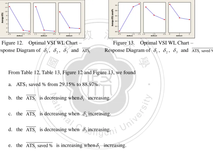
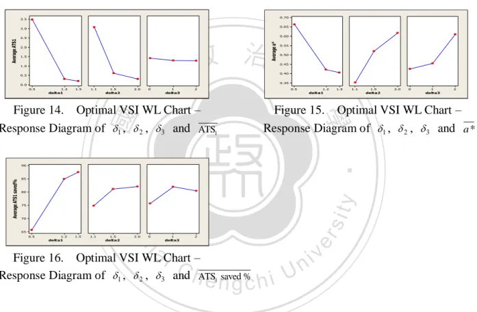
(14) LIST OF FIGURES Figure 1 The Relationship between Target and 0 ..............................................9 Figure 2. The Structure of VP WL Chart.............................................................12. Figure 3. FP WL Chart– Response Diagram of 1 , 2 , 3 and ARL1 ..........19. Figure 4. VSI WL Chart– Response Diagram of 1 , 2 , 3 and ATS1 ........21. Figure 5. VSSI WL Chart –Response Diagram of 1 , 2 , 3 and ATS1 ......23. Figure 6. VSSI WL Chart –Response Diagram of 1 , 2 , 3 and ANOS ....23. Figure 7. VP WL Chart –Response Diagram of 1 , 2 , 3 and ATS1 ..........26. Figure 8. FP WL chart –Response Diagram of 1 , 2 , 3 and ANOS .........26. Figure 9. Optimal FP WL Chart –Response Diagram of 1 , 2 , 3 vs. ARL1. 立. 政 治 大. ‧. ‧ 國. 學. ..............................................................................................................32. io. sit. y. Nat. Figure 10 Optimal FP WL Chart –Response Diagram of 1 , 2 , 3 and a * .... n. al. er. ............................................................................................................32. i n U. v. Figure 11 Optimal FP WL Chart –Response Diagram of 1 , 2 , 3 and. Ch. engchi. ARL1 saved % ......................................................................................32. Figure 12 Optimal VSI WL Chart –Response Diagram of 1 , 2 , 3 vs. ATS1 ...................................................................................................35. Figure 13 Optimal VSI WL Chart –Response Diagram of 1 , 2 , 3 and ATS1 saved % ......................................................................................35. Figure 14.. Optimal VSI WL Chart –Response Diagram of 1 , 2 , 3 vs. ATS1 ...................................................................................................38. XIII.
(15) Figure 15 Optimal VSI WL Chart –Response Diagram of 1 , 2 , 3 and a * ............................................................................................................38 Figure 16 Optimal VSI WL Chart –Response Diagram of 1 , 2 , 3 and ATS1 saved % ......................................................................................38. Figure 17 Optimal VSSI WL Chart –Response Diagram of 1 , 2 , 3 vs. ATS1 ...................................................................................................42. Figure 18 Optimal VSSI WL Chart –Response Diagram of 1 , 2 , 3 and. 政 治 大 Optimal VSSI 立WL Chart –Response Diagram of , , . ATS1 saved % ......................................................................................42. Figure 19. 1. 2. 3. vs.. ‧ 國. 學. ANOS ................................................................................................42. Figure 20 Optimal VSSI WL Chart –Response Diagram of 1 , 2 , 3 and. ‧. ANOS saved % .....................................................................................42. sit. y. Nat. Figure 21 Optimal VSSI WL Chart –Response Diagram of 1 , 2 , 3 vs.. n. al. er. io. ATS1 ...................................................................................................47. i n U. v. Figure 22 Optimal VSSI WL Chart –Response Diagram of 1 , 2 , 3 vs. a *. Ch. engchi. ............................................................................................................47 Figure 23 Optimal VSSI WL Chart –Response Diagram of 1 , 2 , 3 and ATS1 saved % ......................................................................................47. Figure 24 Optimal VSSI WL Chart –Response Diagram of 1 , 2 , 3 v.s. ANOS .................................................................................................48. Figure 25 Optimal VSSI WL Chart –Response Diagram of 1 , 2 , 3 and ANOS saved % .....................................................................................48. Figure 26 Optimal VP WL Chart –Response Diagram of 1 , 2 , 3 vs. ATS1. XIV.
(16) ............................................................................................................52 Figure 27 Optimal VSSI WL Chart –Response Diagram of 1 , 2 , 3 and ATS1 saved % ......................................................................................52. Figure 28 Optimal VP WL Chart –Response Diagram of 1 , 2 , 3 vs.. ANOS ................................................................................................52 Figure 29. Optimal VP WL Chart –Response Diagram of 1 , 2 , 3 and ANOS saved % .....................................................................................52. Figure 30 Optimal VP WL Chart –Response Diagram of 1 , 2 , 3 vs. ATS1. 政 治 大. ............................................................................................................57. 立. Figure 31 Optimal VP WL Chart –Response Diagram of 1 , 2 , 3 and. ‧ 國. 學. ATS1 saved % ......................................................................................57. ‧. Figure 32 Optimal VP WL Chart –Response Diagram of 1 , 2 , 3 vs. a *. sit. y. Nat. ............................................................................................................57. n. al. er. io. Figure 33 Optimal VP WL Chart –Response Diagram of 1 , 2 , 3 vs.. i n U. v. ANOS .................................................................................................58. Ch. engchi. Figure 34 Optimal VP WL Chart –Response Diagram of 1 , 2 , 3 and ANOS saved % .....................................................................................58. Figure 35 The Structure of FP EWMA WL Chart...............................................65 Figure 36 The Structure of VSI EWMA WL Chart.............................................68 Figure 37 FP EWMA WL Chart –Response Diagram of 1 , 2 , 3 v.s. ARL1 under λ = 0.05.....................................................................................73 Figure 38 FP EWMA WL Chart –Response Diagram of 1 , 2 , 3 and ARL1 saved % under λ = 0.05.............................................................73. XV.
(17) Figure 39. FP EWMA WL Chart –Response Diagram of 1 , 2 , 3 v.s. ARL1 under λ=0.1.........................................................................................75. Figure 40 FP EWMA WL Chart –Response Diagram of 1 , 2 , 3 and ARL1 saved % under λ=0.1.................................................................75. Figure 41 FP EWMA WL Chart –Response Diagram of 1 , 2 , 3 v.s. ARL1 under λ=0.15.......................................................................................77 Figure 42 FP EWMA WL Chart –Response Diagram of 1 , 2 , 3 and. 政 治 大. ARL1 saved % under λ=0.15...............................................................77. 立. Figure 43 FP EWMA WL Chart –Response Diagram of 1 , 2 , 3 v.s. ARL1. ‧ 國. 學. under λ=0.2.........................................................................................79. Figure 44 FP EWMA WL Chart –Response Diagram of 1 , 2 , 3 and. ‧. ARL1 saved % under λ=0.2.................................................................79. sit. y. Nat. io. al. er. Figure 45 FP EWMA WL Chart –Response Diagram of 1 , 2 , 3 v.s. ARL1. v. n. under λ=0.25.......................................................................................81. Ch. engchi. i n U. Figure 46 FP EWMA WL Chart –Response Diagram of 1 , 2 , 3 and ARL1 saved % under λ=0.25...............................................................81. Figure 47 FP EWMA WL Chart –Response Diagram of 1 , 2 , 3 v.s. ARL1 under λ=0.3.........................................................................................83 Figure 48 FP EWMA WL Chart –Response Diagram of 1 , 2 , 3 and ARL1 saved % under λ=0.3.................................................................83. Figure 49. FP EWMA WL Chart –Response Diagram of 1 , 2 , 3 v.s. ARL1 under λ=0.4.........................................................................................85. XVI.
(18) Figure 50 FP EWMA WL Chart –Response Diagram of 1 , 2 , 3 and ARL1 saved % under λ=0.4.................................................................85. Figure 51 FP EWMA WL Chart –Response Diagram of 1 , 2 , 3 v.s. ARL1 under λ=0.5.........................................................................................87 Figure 52 FP EWMA WL Chart –Response Diagram of 1 , 2 , 3 and ARL1 saved % under λ=0.5.................................................................87. Figure 53 FP EWMA WL Chart –Response Diagram of 1 , 2 , 3 v.s. ARL1. 政 治 大 FP EWMA立 WL Chart –Response Diagram of , , . under λ=0.6.........................................................................................89. Figure 54. 1. 2. 3. and. ‧ 國. 學. ARL1 saved % under λ=0.6.................................................................89. ‧. Figure 55 FP EWMA WL Chart –Response Diagram of 1 , 2 , 3 v.s. ARL1. y. Nat. under λ=0.7.........................................................................................91. al. er. io. sit. Figure 56 FP EWMA WL Chart –Response Diagram of 1 , 2 , 3 and. n. ARL1 saved % under λ=0.7.................................................................91. Ch. engchi. i n U. v. Figure 57 FP EWMA WL Chart –Response Diagram of 1 , 2 , 3 v.s. ARL1 under λ=0.8.........................................................................................93 Figure 58 FP EWMA WL Chart –Response Diagram of 1 , 2 , 3 and ARL1 saved % under λ=0.8.................................................................96. Figure 59. FP EWMA WL Chart –Response Diagram of 1 , 2 , 3 v.s. ARL1 under λ=0.9.........................................................................................95. Figure 60 FP EWMA WL Chart –Response Diagram of 1 , 2 , 3 and ARL1 saved % under λ=0.9.................................................................95. XVII.
(19) Figure 61 VSI EWMA WL Chart –Response Diagram of 1 , 2 , 3 v.s. ATS1 under λ = 0.05..........................................................................99. Figure 62 VSI EWMA WL Chart –Response Diagram of 1 , 2 , 3 and ATS1 saved % under λ = 0.05.............................................................99. Figure 63 VSI EWMA WL Chart –Response Diagram of 1 , 2 , 3 v.s. ATS1 under λ=0.1............................................................................102. Figure 64 VSI EWMA WL Chart –Response Diagram of 1 , 2 , 3 and. 政 治 大 VSI EWMA 立WL Chart –Response Diagram of , , . ATS1 saved % under λ=0.1...............................................................102. Figure 65. 1. 2. 3. v.s.. ‧ 國. 學. ATS1 under λ=0.2............................................................................105. Figure 66 VSI EWMA WL Chart –Response Diagram of 1 , 2 , 3 and. ‧. ATS1 saved % under λ=0.2...............................................................105. y. Nat. al. er. io. sit. Figure 67 VSI EWMA WL Chart –Response Diagram of 1 , 2 , 3 v.s.. n. ATS1 under λ=0.3............................................................................108. Ch. engchi. i n U. v. Figure 68 VSI EWMA WL Chart –Response Diagram of 1 , 2 , 3 and ATS1 saved % under λ=0.3...............................................................108. Figure 69. VSI EWMA WL Chart –Response Diagram of 1 , 2 , 3 v.s. ATS1 under λ=0.5............................................................................111. Figure 70 VSI EWMA WL Chart –Response Diagram of 1 , 2 , 3 and ATS1 saved % under λ=0.5...............................................................111. Figure 71 VSI EWMA WL Chart –Response Diagram of 1 , 2 , 3 v.s. ATS1 under λ=0.7............................................................................114. XVIII.
(20) Figure 72 VSI EWMA WL Chart –Response Diagram of 1 , 2 , 3 and ATS1 saved % under λ=0.7...............................................................114. Figure 73 VSI EWMA WL Chart –Response Diagram of 1 , 2 , 3 v.s. ATS1 under λ=0.9............................................................................117. Figure 74 VSI EWMA WL Chart –Response Diagram of 1 , 2 , 3 and ATS1 saved % under λ=0.9...............................................................117. Figure 75 The Probability Plot for X................................................................125. 政 治 大 FP EWMA WL Chart........................................................................129 立. Figure 76 FP EWMA WL Control Chart...........................................................127 Figure 77. Figure 78 FP EWMA WL Chart........................................................................131. ‧ 國. 學. Figure 79. VSI EWMA WL Chart......................................................................134. ‧. Figure 80 FP WL Chart.....................................................................................134. sit. y. Nat. Figure 81 VSI WL Chart...................................................................................135. io. er. Figure 82 Optimal VP WL Chart.......................................................................136 Figure 83 Y S 2 Chart......................................................................................137. n. al. Figure 84. Ch. engchi. i n U. v. EWMA Y EWMA ln( S 2 ) Chart.....................................................139. XIX.
(21) CHAPTER 1.. INTRODUCTION. In statistical process control, control charts are used to monitor processes and detect the assignable cause(s) which changed the process mean and variance. Shewhart (1924) first developed the control charts to monitor the process. The Shewhart control charts have been widely used for industrial processes ever since. An X chart is usually used to monitor the process mean and an S (or R ) chart is used. to monitor the variation of a process. However Shewhart charts are insensitive in. 政 治 大 (CUSUM) chart to combat this drawback. Then in 1959 Roberts (1959) introduced the 立 detecting small shifts, in 1954, Page (1954) first introduced the cumulative sum. exponentially weighted moving average (EWMA) control chart to detect small shifts in. ‧ 國. 學. the process mean.. ‧. When dealing with a quality characteristic of a variable, it is usually necessary to. sit. y. Nat. monitor both the mean value and its variability simultaneously. Two control charts are. io. er. usually required to monitor the process mean and the process variability respectively. Shewhart’s X S or X R control charts are the common choices, in which X. al. n. v i n chart monitors the process meanC while S (or R ) chart h e n g c h i U monitors the variation.. However, this approach is laborious and time-consuming. Hence, it is advantageous to consider using a single chart based on only one statistic to monitor the process mean and the variation simultaneously. In recent years, a few researchers had proposed different types of single charts that jointly monitor the process mean and the variation. They are of Shewhart-types, EWMA-types and CUSUM-types. Chen and Cheng (1998) proposed the Max chart which has effectively combined the X chart and S chart into one single chart. The main advantage of the Max chart is that one can monitor both the process mean and the process variance by looking at one chart. Chao and Cheng (1996) developed the 1.
(22) Semicircle (SC) chart. This chart combines the detection of the mean shift and the variability change into one chart, and is simple to use and easy to understand. The advantage of the SC chart is that it is easy to attribute an out-of-control signal to the cause of the mean shift or/and the variability change. However, the SC chart is insensitive to small changes within a process. In order to improve the SC chart, Chen et al. (2004) used the statistic of the SC chart to construct a new chart, EWMA-SC chart. This chart not only could monitor both the process mean and the process variance simultaneously, but also it is sensitive to small changes in the mean shift or/and the. 政 治 大 assignable causes that had shifted the process mean but did not change the process 立 variability. However, the EWMA-SC chart is slow in detecting the most common. variance. In order to improve this chart’s deficiency, Costa and Rahim (2006). ‧ 國. 學. introduced a new statistic to construct an EWMA chart that gave better overall. ‧. performance. Khoo, Wu, Chen and Yeong (2010) proposed a single EWMA X R. io. er. simultaneously and identifies the source of the signal(s).. sit. y. Nat. chart by combining the X and R charts which monitors the mean and variance. Loss function is used broadly in industry to measure the cost due to poor quality.. al. n. v i n C hthe loss chart basedUon the concept of the loss Several researchers have developed engchi. function. From Cyrus (1997), the average loss L is proportional to the sum of squares of the deviations of the quality characteristic from the in-control process mean. Wu and Tian (2006) proposed the weighted loss function chart based on the average weighted loss function which uses a weighted factor to adjust the weight of the loss due to the square of the mean shift and the variance change. This single chart is able to monitor the mean shift and the variance increase simultaneously and is more powerful than the. X S chart. However, they assumed that the process mean was target. The charts mentioned above are monitoring a process with a fixed sampling interval, sample size and control limits. Their effectiveness for detecting process shifts 2.
(23) in mean and variance becomes less for today’s manufacturing environment. A method to improve the problem is to construct the adaptive control charts. Reynolds et al. (1988) and Chengalur et al. (1989) first studied the use of X charts with variable sampling intervals (VSI) to detect mean shifts. Prabhu et al. (1994) studied the propertied of the X chart with both the sample sizes and the sampling intervals variable (VSSI). Costa (1999a) proposed a variable parameters (VP) X chart which all design parameters were variable, including sample size, sampling intervals and control limit coefficient. Costa and De Magalhaes (2007) investigated the performance. 政 治 大 schemes for monitoring mean and variance in two dependent process steps. Ko and 立. of X-bar and R charts with VSSIs. Yang and Su (2007) addressed the adaptive control. Yeh (2010) studied the effect of VSI economic chart with minimum average loss. Yang. ‧ 國. 學. and Chen (2010) proposed VSI mean and variance control charts to monitor dependent. ‧. process steps.. sit. y. Nat. Some researches of using a single chart to monitor the mean and variance. io. er. simultaneously with the adaptive control schemes had been studied in recent years. Wu, Tian and Zhang (2005) proposed a control chart based on the average weighted loss. al. n. v i n C hZhang and Wu (2006) function (WLF) with VSSI scheme. use the average weighted engchi U loss function to construct a new chart with CUSUM scheme and with variable. sampling intervals. Wu, Zhang and Wang (2007) proposed a VSSI WLF chart which is a CUSUM chart based on the weighted loss function with VSSI scheme. Yang and Lin (2009) proposed a New VP Loss function chart allowing process mean not to be the target. In this project, we propose a new chart -- the weighted average loss (WL) chart to monitor the two-sided mean shifts and the variance changes while the target value may be different from the in-control mean. The WL chart’s monitoring statistic WL is derived from Taguchi’s (1986) loss function. This statistic applied a weighted factor to 3.
(24) adjust the weights of the loss due to the square of the deviation of the process mean from the target and the variance change. We described the derivation in chapter 2. The difference of the statistics between the WL chart and Wu’s weighted loss function chart is that the in-control mean may not equal to the target in the WL chart but equal to target in Wu’s. The fixed parameters (FP) WL chart monitors a process with fixed sampling interval, sample size and false alarm rate. Based on the WL, we also developed the adaptive charts (VSI WL chart, VSSI WL chart and VP WL chars). The VSI WL chart. 政 治 大 and sample sizes. The VP WL chart uses variable sampling intervals, sample sizes and 立 uses variable sampling intervals. The VSSI WL chart uses variable sampling intervals. false alarm rates. We also proposed the optimal adaptive WL charts using an. ‧ 國. 學. optimization technique. In addition, in order to detect the small shifts of the process. n. al. er. io. sit. y. Nat. scheme further.. ‧. mean and variance effectively, we also construct the WL charts using the EWMA. Ch. engchi. 4. i n U. v.
(25) CHAPTER 2.. THE DISTRIBUTION OF THE WEIGHTED AVERAGE LOSS. 2.1 Taguchi Loss Function and its Expectation and Estimator Taguchi (1986) claimed that “quality is the loss a product causes to society after being shipped, other than any losses caused by its intrinsic functions”. Furthermore Taguchi quantifies the deviations of a product characteristic from the target in terms of monetary units by using a quadratic loss function defined as L( X ) K ( X T ) 2. (1). 政 治 大 loss coefficient. We can derive the expectation of the loss function to explain the 立. where X is the quality characteristic, T is the target value for X and K is the quality. 學. ‧ 國. average loss per unit product from equation (1), that is E ( L) E K ( X T ) 2 . ‧. K 2 ( T ) 2 . Nat. n. sit er. io. al. y. where and 2 are the mean and variance of X.. i n U. v. 2.2 The Estimator of the Expectation of the Loss Function and Weighted Average Loss. Ch. engchi. Since the mean and the variance of a process are usually unknown, so is the average loss function. Hence we have to estimate it and the estimator is proportional to the sum of squares of the deviations of the quality characteristic X from the target, i.e. n. ^. E ( L) . (X i 1. i. T )2 . n. n 1 2 S ( X T )2 . n. (2). It is clear that the estimator comprises the sample variance and the square deviation of the sample mean from the target. We now would modify the estimator of the average loss function (eq. (2)) to a 5.
(26) weighted average loss (WL), that is WL aS 2 (1 a)( X T ) 2. (3). where the weighting factor “a” ( 0 a 1 ) is used to adjust the weight of the loss due to the variance shift and the square of the mean shift from the target. We will use the weighted average loss (WL) to construct the WL control chart. The chart could monitor the mean shift from the process target and the variance change simultaneously.. 2.3 The Approximate Distribution of Weighted Average Loss In order to construct control chart based on WL, we need to find the distribution. 政 治 大. of the WL statistic. Since we can’t get the exact expression of this distribution, we. 立. would apply Patnaik’s (1949) and Moschopoulos and Canada’s (1984) results to get the. ‧ 國. 學. approximate distribution of WL. Patnaik (1949) illustrated the transformation of a non-central chi-square distribution to a central chi-square distribution. Moschopoulos. ‧. and Canada (1984) proposed a method to get the approximate cumulative probability. y. Nat. n. al. er. io. (see Appendix 1).. sit. function (c.d.f.) for the linear combination of the central chi-square random variables. i n U. v. Assume X follows a normal distribution with mean and variance 2 , that is. Ch. engchi. X ~ N ( , ) . The weighted average loss (WL) (eq. (3)) is 2. WL aS 2 (1 a)( X T ) 2. where 0 a 1 . Since. (n 1 ) S 2. . 2. ~ 2( n 1 ). (4). where 2( n1) is a central chi-square distribution with (n–1) degrees of freedom,. n( X T )2. . 2. ~ 21,. (5). where 21, is a non-central chi-square distribution with 1 degree of freedom and a 6.
(27) non-centrality parameter , . n( T )2. .. 2. From equations (4) and (5),. 2. 2. S ~. (n 1). (X T) ~ 2. 2 ( n 1). 2 n. (6). 21,. (7). And then. 2. WL aS 2 (1 a)( X T ) 2 ~ a. (n 1). 2( n 1) (1 a). 2 n. 21,. 政 治 大 chi-square distribution. However, 立 its exact distribution is untractable. We would try to which is a linear combination of a central chi-square distribution and a non-central. ‧ 國. 學. find its approximate distribution.. The following steps show how to find the approximate c.d.f. of WL:. ‧. Step 1. Use Patnaik’s method to transform a non-central chi-square distribution. sit. y. Nat. into a central chi-square distribution.. n. al. er. io. Transform equation (5) to a central chi-square distribution using Patnaik’s method (1949):. Ch. e ngc h~i. n( X T ) 2. 2 1,. 2. i n U. v. 2. . (v). where 2(v ) is a central chi-square distribution with v degree of freedom, and. 1. 1. and v 1 . 2 1 2. .. The distribution of ( X T ) 2 is derived as. ( X T )2 ~. 2 n. 2( v ). (8). From equations (6) and (8), we have WL aS (1 a)( X T ) ~ a 2. 2. 2. (n 1). . 2. ( n 1). (1 a). 2 n. which is a linear combination of central chi-square random variables. 7. 2(v ).
(28) Step 2. Use the method of Moschopoulos and Canada (1984) to obtain the approximate distribution of WL. The distribution of WL statistic is a linear combination of central chi-squares: WL ~ a. Let c1 a. 2 (n 1). , c2 (1 a ). 2 (n 1). 2 n. 2( n 1) (1 a). 2. 2(v ). n. (9). , v1 n 1 and v2 v .. Using the method of Moschopoulos and Canada (1984) (See Appendix 1), WL is approximate the distribution of Q with parameters n and . That is,. 立. 政WL ~ Q治. 大. (10). n ,. w. 0. j 0. (11). ‧. ‧ 國. Fn, ( x) P(WL x) b2 a j g j ( y )dy. Nat. y. y s j 1e y / 2 c1 is the p.d.f. of Gamma distribution, ( s j , 2c1 ) , (2c1 ) s j ( s j ). io. sit. where g j ( y ) . . 學. The c.d.f. of Qn , (Moschopoulos and Canada (1984)) is. er. with the shape parameter s j and scale parameter 2c1 , and s m1 m2 ,. n. al. i n Ch (m ) (1 cU/ c ) , jn ) g c h i with A(ce j!. v. j. b2 (. c1 m2 ) , a j A(c2 , j ) c2. m2 . v2 and (mi ) r mi (mi 1) (mi r 1) . 2. i. j. 1. i. i. for j = 0, 1, 2…, m1 . v1 , 2. Now we will give the in-control process and out-of-control process distributions of X, and derive the c.d.f. of the statistic WL. For the In-control process: X ~ N (0 , 02 ). Let the process target be T, and T 0 3 0 , 3 0 . 8. (12).
(29) The relationship of T and 0 is shown in figure 1 below:. The Relationship between the Target and 0. Figure 1.. 政 治 大 立WL aS (1 a)( X T ). Following (9), we get the distribution of WL below:. 02. (n 1). . 2. ( n 1). (1 a). 0 2 0 n. 2( v ) 0. (13). ‧. 02 n( 0 T ) 2 0 n 32 . , v0 1 and 0 2 1 2 0 0 1 0. al. n. WL ~ Qn , 0 .. Ch. The c.d.f. of Cn , 0 is. engchi. er. io. sit. y. Nat. Hence,. ~a. 2. 學. where 0 1 . ‧ 國. 2. i n U. Fn, 0 ( x) P(WL x | WL ~ Qn, 0 ) For the out-of-control process: X ~ N (1 , 12 ). where 1 0 1 0 , 1 0 and 12 22 02 , 2 1 . The distribution of WL is then WL aS 2 (1 a)( X T ) 2. 9. v. (14).
(30) ~a. 12 (n 1). 2( n 1) (1 a). 12 1 n. 2(v ). (15). 1. 2. n( 0 1 0 T )2 * *2 * , v1 1 and where 1 1 n 1 3 . * * 2 2 2 0 1 1 2 2 Hence,. WL ~ Qn*, * . The c.d.f. of Qn*, * is. (16). 政 治 大. Fn*, * ( x) P(WL x | WL ~ Qn*, * ). 立. (17). ‧. ‧ 國. 學. n. er. io. sit. y. Nat. al. Ch. engchi. 10. i n U. v.
(31) CHAPTER 3.. DESIGN AND ARL ANALYSIS OF THE FP, VSI, VSSI AND VP WL CHARTS. 3.1. Design of the FP WL Chart The FP (fixed parameters) WL chart uses fixed sampling interval h0, sample size. n0 and false alarm rate 0 . From (14), the upper control limit (UCL) and lower control limit (LCL) of the FP WL chart are: UCL Fn0 1, 0 (1 . 0 2. ),. 政 治2 ) . 大. LCL Fn0 1, 0 (. 立. 0. The performance of a control chart can be measured by the average run length. ‧ 國. 學. (ARL), which is the average number of samples required to get the first signal. The out-of-control ARL1 is used to measure the detection effectiveness of the control chart. ‧. and the in-control ARL0 measures the false alarm rate. When the process is. y. Nat. sit. out-of-control, the ARL1 is calculated by:. n. al. er. io. 1 1 P( LCL WL UCL | WL ~ Qn* , * ). Ch. n U e n g c2h i. 1 Fn* , * ( Fn1, 0 (1 0. 0. 0. Ideally ARL1 should be as small as possible.. 11. 0. )) Fn* , * ( Fn0 1, 0 (. Then. ARL1 . iv. 1 1 . 0. 0 2. )) ..
(32) 3.2. Design of the VP WL Control Chart The VP (variable parameters) WL chart uses variable sampling intervals hq,. sample sizes nq and false alarm rates q , q = 1, 2. It has the warning limits (UWLq and LWLq) and the control limits (UCLq and LCLq) that divide the chart into three regions: central region, warning region and action region, see Figure 2.. 政 治 大. 立. ‧. ‧ 國. 學. Figure 2.. The Structure of VP WL Chart. sit. y. Nat. n. al. er. io. Let h0, n0 and 0 are the sampling interval, sample size and false alarm rate for. i n U. v. FP WL chart. The variable sampling intervals hq, sample sizes nq and false alarm rate. Ch. engchi. q , q = 1, 2, are adopted where 0 h2 h0 h1 , 0 n1 n0 n2 , 0 1 0 2 . From (14), the UCLq and LCLq of the VP chart are. UCLq Fnq 1, q (1 LCLq Fnq 1, q (. q. q 2. 2. ). ). where q nq 32 ,q=1,2. If the statistic WL falls into the central region, the next sampling interval should be long, sample size should be small and false alarm rate should be small, (h1, n1,. 1 ),with corresponding control limits (UCL1, LCL1) and warning limits (UWL1, LWL1) 12.
(33) for the next sample. If WL falls into the warning region, the next sampling interval should be short, sample size should be large and false alarm rate should be large, (h2, n2, 2 ), with corresponding control limits (UCL2, LCL2) and warning limits (UWL1, LWL1). If WL falls into the action region, an out-of-control signal would have occurred. In order to compare the performance of VP and FP chart, we should demand the same average sampling interval, sample size and false alarm rate when the process is in-control process. That is, p1h1 (1 p1 )h2 h0. 立. (18). 1h1 (1 p1 ) 2 0. (20). 1 1. 1. 2. (19). 0. ‧ 國. 學. where. 治 政 p n (1 p )n n 大. ‧. p1 P( LWLq WL UWLq | LCLq WL UCLq ,WL ~ Qnq , q ) , q = 1, 2.. y. sit. n. al. The derivation of the warning limits is as follows:. Ch. engchi. er. io. process.. Nat. which is the probability of the WL falls in the central region under the in-control. i n U. v. Specify n0 , n1 , n2 , h0 , h2 , 0 and 1 , we could calculate the value of p1 from (19):. p1 . n0 n2 n1 n2. and the values of the h1 and 2 : From (18) and (19),. h1 . h0 (n2 n1 ) h2 (n0 n1 ) . n2 n0. From (19) and (20),. 2 . 0 (n1 n2 ) 1 (n0 n2 ) n1 n0. .. Let the cumulative probability of the center line (CL) be p* , that is 13.
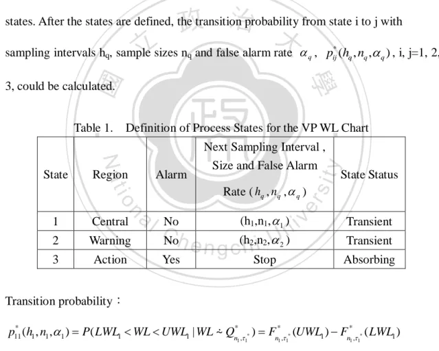
(34) Fnq , q (CLq ) p* , q = 1, 2. (21). and let the probability of WL falling between LWLq and CLq equal to the probability of WL falling between CLq and UWLq, i.e.. P( LWLq WL CLq | WL ~ Qnq , q ) P(CLq WL UWLq | WL ~ Qnq , q ). (22). Hence. p1 P( LWLq WL UWLq | LCLq WL UCLq ,WL ~ Qnq , q ) . P( LWLq WL UWLq | WL ~ Qnq , q ) P( LCLq WL UCLq | WL ~ Qnq , q ). That is,. 政 治 大. 立. ‧. ‧ 國. From (22),. 學. P( LWLq WL UWLq | WL ~ Qnq , q ) P( LCLq WL UCLq | WL ~ Qnq , q ) p1. P( LWLq WL CLq | WL ~ Qnq , q ) P(CLq WL UWLq | WL ~ Qnq , q ) (1 q ) p1. sit. y. Nat. Then,. n. al. er. io. P( LWLq WL CLq | WL ~ Qnq , q ) (1 q ) . Ch. P(CLq WL UWLq | WL ~ Qnq , q. engchi. q. Fnq , q (CLq ) Fnq , q ( LWLq ) (1 q ) . p1 2. Hence, the LWL could be derived as LWLq Fnq 1, q ( Fnq , q (CLq ) (1 q ) . From eq. (21), Fnq , q (CLq ) p* , LWLq Fnq 1, q ( p* (1 q ) . 14. (23). 1. (24). iv p n )U (1 ) . Simplify (23),. Similarly, we could derive the UWLq. p1 2. p1 ) 2. p1 ) 2. 2.
(35) UWLq Fnq 1, q ( p* (1 q ) . p1 ) 2. The performance of a control chart could be measured by the average time to signal (ATS1), which is the average time required to signal a process shift after it has occurred. The ATS0 is the average time until a false alarm occurred. Apply the Markov chain approach to derive the ATS1, and all possible process states are defined in Table 1. Table 1 shows the 3 possible process states based on Markov property. States 1 and 2 are transient states since they may transit from one to other states, while state 3 is an absorbing state because it cannot transit to any other. 政 治 大. states. After the states are defined, the transition probability from state i to j with. 立. sampling intervals hq, sample sizes nq and false alarm rate q , pij* (hq , nq , q ) , i, j=1, 2,. ‧ 國. 學. 3, could be calculated.. ‧. Table 1.. Alarm. Rate ( hq , nq , q ). al. n. Central. 2. Warning. 3. Action. i n C ) Noh e n g c(hh,ni ,U (h1,n1, 1 ). No. 2. Yes. 2. State Status. er. io. 1. y. Region. Next Sampling Interval , Size and False Alarm. sit. Nat. State. Definition of Process States for the VP WL Chart. v. Transient Transient. 2. Stop. Absorbing. Transition probability: * p11 (h1 , n1 , 1 ) P( LWL1 WL UWL1 | WL ~ Qn* , * ) Fn* , * (UWL1 ) Fn* , * ( LWL1 ) 1. 1. 1. 1. 1. 1. * p12 (h1 , n1 , 1 ) P( LCL1 WL LWL1 or UWL1 WL UCL1 | WL ~ Qn* , * ) 1. 1. ( Fn* , * ( LWL1 ) Fn* , * ( LCL1 )) ( Fn* , * (UCL1 ) Fn* , * (UWL1 )) 1. 1. 1. 1. 1. 1. 1. 1. * p13 (h1 , n1 , 1 ) 1 P( LCL1 WL UCL1 | WL ~ Qn* , * ) 1 ( Fn* , * (UCL1 ) Fn* , * ( LCL1 )) 1. 1. 1. 1. 1. 1. * p21 (h2 , n2 , 2 ) P( LWL2 WL UWL2 | WL ~ Qn* , * ) Fn* , * (UWL2 ) Fn* , * ( LWL2 ) 2. 15. 2. 2. 2. 2. 2.
(36) * p22 (h2 , n2 , 2 ) P( LCL2 WL LWL2 or UWL2 WL UCL2 | WL ~ Qn* , * ) 2. 2. ( Fn* , * ( LWL2 ) Fn* , * ( LCL2 )) ( Fn* , * (UCL2 ) Fn* , * (UWL2 )) 2. 2. 2. 2. 2. 2. 2. 2. * p23 (h2 , n2 , 2 ) 1 P( LCL2 WL UCL2 | WL ~ Qn* , * ) 1 ( Fn* , * (UCL2 ) Fn* , * ( LCL2 )) 2. 2. 2. 2. 2. 2. * * * p31 p32 0 , p33 1. The transition probability from state i to j can be expressed by a square matrix. p11* * P* p21 0 . * p13 * p23 , 1 . * p12 * p22 0. 政 治 大 The transition probability matrix which contains the transient probability from 立. ‧ 國. p12* * . p22 . ‧. p* Q* 11 * p21. 學. transient state i to transient state j. sit. y. Nat. The ATS1 is derived as. io. n. al. er. ATS1 r* (I Q* ) 1 h ,. i n U. v. where I is the identity matrix of order 2, h' (h1 , h2 ) is a (1x2) vector of sampling. Ch. engchi. time for transient state i, i = 1, 2, r* (r1* , r2* ) is a (1x2) vector with the steady-state starting probability, ri* , i=1, 2, for transient state i. The ri* can be obtained by solving the equation. r*Q* r* and. 2. r i 1. i. *. 1. That is,. 1 r1* . 1. * 11. p11* p11* p12* * 21. p p * * * * and p11 p12 p21 p22 16. r2* . * p21 * * p21 p22. 1. * p11* p21 . * * p11* p12* p21 p22.
(37) We also use the average number of observations to signal (ANOS) to measure the performance of a control chart, which ANOS is the average number of observations required to signal a process shift after it has occurred. It is derived as. ANOS r* (I Q* )1 n ,. (25). where n (n1 , n2 ) is a (1x2) vector of sample size for transient state i, i=1,2. When 1 0 2 , the VP design can reduce to the VSSI design. The derivation of the control limits and warning limits and the calculation of the ATS 1 and ANOS are the same as the VP chart.. 政 治 大. When 1 2 0 and n1 n2 n0 , the VP design can reduce to the VSI. 立. 學. h0 h2 is calculated from (18). The derivation of the control limits h1 h2. ‧ 國. design where p1 . and warning limits and the calculation of the ATS 1 are the same as the VP chart.. ‧. ATS1 Analysis and ATS1 Comparison among the FP, Specified VSI, VSSI. sit. y. Nat. 3.3. io. er. and VP WL Charts (1) ARL1 Analysis of FP WL Chart. n. al. Under 0 0 , 02 1 ,. i n C n h 5 , h 1 , 0U e n g c h i .0027 0. 0. 0. v. (or ARL0 = 370.37) and. a 0.6 . Consider the levels of the parameters, 1 = (0.5, 1.2, 1.5), 2 = (1.1, 1.5, 2). and 3 = (0, 1, 2). The 27 combinations of 1 , 2 and 3 are arranged by Orthogonal Arrays (O.A.) L27(313). The ARL1s of the 27combinations of the FP chart are listed in Table 2.. 17.
(38) Table 2.. ARL1 for FP WL Chart. 1. 2. 3. ARL1. ANOS. No.. 1. 2. 3. ARL1. ANOS. 1. 0.5. 1.1. 0. 109.54. 547.70. 16. 1.2. 2. 0. 1.88. 9.41. 2. 0.5. 1.1. 1. 38.67. 193.35. 17. 1.2. 2. 1. 1.59. 7.96. 3. 0.5. 1.1. 2. 29.36. 146.81. 18. 1.2. 2. 2. 1.63. 8.12. 4. 0.5. 1.5. 0. 7.79. 38.93. 19. 1.5. 1.1. 0. 9.86. 49.32. 5. 0.5. 1.5. 1. 5.90. 29.51. 20. 1.5. 1.1. 1. 2.70. 13.51. 6. 0.5. 1.5. 2. 6.20. 31.02. 21. 1.5. 1.1. 2. 2.04. 10.19. 7. 0.5. 2. 0. 2.36. 11.80. 22. 1.5. 1.5. 0. 3.01. 15.07. 8. 0.5. 2. 1. 2.31. 11.55. 23. 1.5. 1.5. 1. 1.79. 8.97. 9. 0.5. 2. 2. 2.66. 13.32. 24. 1.5. 1.5. 2. 1.64. 8.18. 10. 1.2. 1.1. 0. 21.67. 0. 1.67. 8.34. 11. 1.2. 1.1. 1. 5.10. 1.39. 6.97. 12. 1.2. 1.1. 2. 立 3.60. 1 2. 1.39. 6.95. 13. 1.2. 1.5. 0. 4.14. 20.72. 14. 1.2. 1.5. 1. 2.42. 12.09. 15. 1.2. 1.5. 2. 2.21. 11.05. 108.35 治 25 1.5 2 政 25.51 26 1.5大 2 17.99. 27. 1.5. 2. 學 ‧. ‧ 國. No.. y. Nat. In order to compare the ANOS among FP, VSSI and VP charts later, we have to. er. io. sit. calculate the ANOS of FP chart by letting n1 = n2 = n0 and 1 2 0 in the. al. equation (25) of the VP design.. n. v i n To investigate the effect of C ,h and on the e n g c h i UARL , the response table and 1. 1. 3. 2. response diagram show the results of the sensitivity analysis (Table 3 and Figure 3).. Table 3.. FP WL Chart– Response Table of 1 , 2 , 3 and 1. ARL1. 2. ARL1. 3. ARL1. 0.5. 22.76. 1.1. 24.73. 0. 17.99. 1.2. 4.92. 1.5. 3.90. 1. 6.88. 1.5. 2.83. 2. 1.88. 2. 5.64. 18. ARL1.
(39) 25. Average ARL1. 20. 15. 10. 5. 0 0.5. 1.2. 1.5. 1.1. delta1. Figure 3.. 1.5. 2.0. 0. 1. delta2. 2. delta3. FP WL Chart– Response Diagram of 1 , 2 , 3 and. ARL1. From Table 3 and Figure 3, we found the average ARL1 a. is decreasing when 1 increasing, b. is decreasing when 2 increasing, c. is decreasing when 3 increasing 3 .. 立. 政 治 大. (2) ATS1 Analysis of VSI WL Chart and ATS1 Comparison between FP WL. ‧ 國. 學. Chart and Specified VSI WL Chart. ‧. Under 0 0 , 02 1 , n0 5 , h0 1 , 0 0.0027 (or ARL0 = 370.37) and. sit. y. Nat. a 0.6 . Consider the levels of the parameters, 1 = (0.5, 1.2, 1.5), 2 = (1.1, 1.5, 2),. n. al. er. io. 3 = (0, 1, 2), (h2, h1) = (0.2, 2), (0.5,1.5), (0.8, 1.2) and p* (0.4, 0.5, 0.6) . The 27. i n U. v. combinations are arranged by L27(313). The ATS1s of the 27combinations of the VSI chart are listed in Table 4.. Ch. engchi. 19.
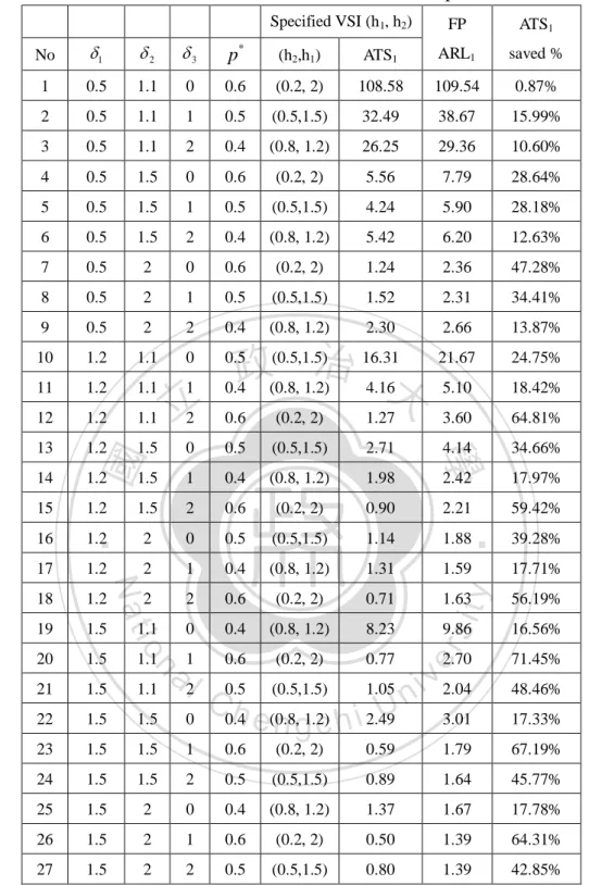
(40) Table 4.. ATS1 for VSI WL Chart and ATS1 saved % Compared to FP WL Chart Specified VSI (h1, h2). FP. ATS1. ATS1. ARL1. saved %. No. 1. 2. 3. p. 1. 0.5. 1.1. 0. 0.6. (0.2, 2). 108.58. 109.54. 0.87%. 2. 0.5. 1.1. 1. 0.5. (0.5,1.5). 32.49. 38.67. 15.99%. 3. 0.5. 1.1. 2. 0.4. (0.8, 1.2). 26.25. 29.36. 10.60%. 4. 0.5. 1.5. 0. 0.6. (0.2, 2). 5.56. 7.79. 28.64%. 5. 0.5. 1.5. 1. 0.5. (0.5,1.5). 4.24. 5.90. 28.18%. 6. 0.5. 1.5. 2. 0.4. (0.8, 1.2). 5.42. 6.20. 12.63%. 7. 0.5. 2. 0. 0.6. (0.2, 2). 1.24. 2.36. 47.28%. 8. 0.5. 2. 1. 0.5. (0.5,1.5). 1.52. 2.31. 34.41%. 9. 0.5. 2. 2. 0.4. (0.8, 1.2). 2.30. 2.66. 13.87%. 10. 1.2. 1.1. 0. 0.5. 21.67. 24.75%. 11. 1.2. 1.1. 1. 5.10. 18.42%. 12. 1.2. 1.1. 13. 1.2. 1.5. 1.2. 1.27. 3.60. 64.81%. 0. 0.5. (0.5,1.5). 2.71. 4.14. 34.66%. 1.5. 1. 0.4. (0.8, 1.2). 1.98. 2.42. 17.97%. 1.2. 1.5. 2. 0.6. (0.2, 2). 0.90. 2.21. 59.42%. 1.2. 2. 0. 0.5. (0.5,1.5). 1.14. 1.88. 39.28%. 1.2. 2. 1. 0.4. (0.8, 1.2). 1.31. 1.59. 17.71%. 1.63. y. 56.19%. 9.86. 16.56%. 2. 2. 0.6. (0.2, 2). 0.71. 19. 1.5. 1.1. 0. 0.4. (0.8, 1.2). 8.23. 20. 1.5. 1.1. 0.6. (0.2, 2). 0.77. 21. 1.5. 1.1. a 12l. 22. 1.5. 1.5. 23. 1.5. 24. n. 1.2. io. Nat. 18. sit. (0.2, 2). er. 17. 0.6. ‧ 國. 16. (0.5,1.5) 治 16.31 政 0.4 (0.8, 1.2) 4.16大. ‧. 15. (h2,h1). 學. 14. 立2. *. n U 0.4 e (0.8, 1.2) 2.49 ngchi. i v 2.04. 2.70. 71.45%. 3.01. 17.33%. (0.5,1.5). 0. C0.5h. 1.5. 1. 0.6. (0.2, 2). 0.59. 1.79. 67.19%. 1.5. 1.5. 2. 0.5. (0.5,1.5). 0.89. 1.64. 45.77%. 25. 1.5. 2. 0. 0.4. (0.8, 1.2). 1.37. 1.67. 17.78%. 26. 1.5. 2. 1. 0.6. (0.2, 2). 0.50. 1.39. 64.31%. 27. 1.5. 2. 2. 0.5. (0.5,1.5). 0.80. 1.39. 42.85%. Note: ATS1 saved % =. 1.05. FP-ARL VSI-ATS 1. 1. 48.46%. FP- ARL1 %. To investigate the effect of 1 , 2 and 3 on the ATS1, the response table and response diagram show the results of the sensitivity analysis (Table 5 and Figure 4).. 20.
(41) Table 5.. VSI WL Chart– Response Table of 1 , 2 , 3 and 1. ATS1. 2. ATS1. 3. ATS1. 0.5. 22.76. 1.1. 24.73. 0. 17.99. 1.2. 4.92. 1.5. 3.90. 1. 6.88. 1.5. 2.83. 2. 1.88. 2. 5.64. ATS1. 25. Average ARL1. 20. 15. 10. 5. 0 0.5. 1.2. 1.5. 1.1. delta1. Figure 4.. 1.5. 2.0. delta2. 0. 1. 2. delta3. VSI WL Chart– Response Diagram of 1 , 2 , 3 and. ATS1. 政 治 大. From Table 4, Table 5 and Figure 4, we found. 立. a. ATS1 saved % from 0.87% to 71.45%. ‧ 國. 學. b. the ATS1 is decreasing when 1 increasing.. ‧. c. the ATS1 is decreasing when 2 increasing.. Nat. sit er. io. al. y. d. the ATS1 is decreasing when 3 increasing.. v. n. (3) ATS1 Analysis of VSSI WL Chart and ATS1 Comparison between FP WL. Ch. engchi. Chart and specified VSSI WL Chart. i n U. Under 0 0 , 02 1 , n0 5 , h0 1 , 0 0.0027 (or ARL0 = 370.37), p * 0.5 and a 0.6 . Consider the levels of the parameters, 1 = (0.5, 1.2, 1.5),. 2 = (1.1, 1.5, 2), 3 = (0, 1, 2), h2 = (0.1, 0.5, 0.9) and (n1, n2): (2, 6), (3, 10), (4, 20). The 27 combinations are arranged by L27(313). The ATS1s of the 27combinations of the VSSI chart are listed in Table 6.. 21.
(42) Table 6.. ATS1 and ANOS for VSSI WL Chart and ATS1 Saved % and ANOS Saved % Compared to FP WL Chart ATS1. ANOS. 1. 2. 3. (n1 , n2 ). h2. h1. ATS1. ANOS. ARL1. ANOS. saved %. saved %. 1. 0.5. 1.1. 0. (2,6). 0.1. 3.70. 93.73. 551.38. 109.54. 547.70. 14.44%. -0.67%. 2. 0.5. 1.1. 1. (3,10). 0.5. 1.20. 21.84. 169.04. 38.67. 193.35. 43.53%. 12.57%. 3. 0.5. 1.1. 2. (4,20). 0.9. 1.01. 12.55. 104.90. 29.36. 146.81. 57.26%. 28.55%. 4. 0.5. 1.5. 0. (2,6). 0.5. 2.50. 5.00. 38.35. 7.79. 38.93. 35.84%. 1.48%. 5. 0.5. 1.5. 1. (3,10). 0.9. 1.04. 3.40. 28.80. 5.90. 29.51. 42.37%. 2.39%. 6. 0.5. 1.5. 2. (4,20). 0.1. 1.06. 2.02. 32.83. 6.20. 31.02. 67.45%. -5.83%. 7. 0.5. 2. 0. (2,6). 0.9. 1.30. 1.94. 12.06. 2.36. 11.80. 18.00%. -2.19%. 8. 0.5. 2. 1. (3,10). 0.1. 1.36. 0.53. 13.73. 2.31. 11.55. 77.05%. -18.90%. 9. 0.5. 2. 2. (4,20). 0.5. 13.32. 54.40%. -52.90%. 10. 1.2. 1.1. 0. (4,20). 108.35. 78.69%. 45.04%. 11. 1.2. 1.1. 1. (2,6). 1.22 治20.37 2.66 政 1.06 4.62 59.55 大 21.67 0.1 2.09 22.78 0.5立2.50 5.10. 25.51. 59.12%. 10.71%. 12. 1.2. 1.1. 2. (3,10). 0.9. 1.04. 1.39. 14.94. 3.60. 17.99. 61.50%. 16.92%. 13. 1.2. 1.5. 0. (4,20). 0.5. 1.03. 1.18. 22.93. 4.14. 20.72. 71.58%. -10.67%. 14. 1.2. 1.5. 1. (2,6). 0.9. 1.30. 1.86. 12.02. 2.42. 12.09. 23.08%. 0.55%. 15. 1.2. 1.5. 2. (3,10). 0.1. 1.36. 0.25. 12.63. 2.21. 11.05. -14.23%. 16. 1.2. 2. 0. (4,20). 0.9. 1.01. 1.06. 19.04. 1.88. ‧. 88.60%. 9.41. 43.47%. -102.28%. 17. 1.2. 2. 1. (2,6). 0.1. 3.70. 0.30. 8.44. 1.59. 7.96. 81.01%. -6.00%. 18. 1.2. 2. 2. (3,10). 0.5. 1.20. 0.68. 11.10. 1.63. 8.12. 57.93%. -36.68%. 19. 1.5. 1.1. 0. (3,10). 0.1. 1.36. 1.06. 31.23. 9.86. 49.32. 89.28%. 36.67%. 20. 1.5. 1.1. 1. (4,20). 80.37%. -48.44%. 1.5. 1.1. 2. (2,6). 10.19. 27.32%. 3.36%. 22. 1.5. 1.5. 0. (3,10). 0.5. 1.20. n U 1.48 9.84 2.04 engchi. 13.51. 21. a 0.5 l 1.03 C 1.30 h 0.9. 23. 1.5. 1.5. 1. (4,20). 0.9. 24. 1.5. 1.5. 2. (2,6). 25. 1.5. 2. 0. 26. 1.5. 2. 27. 1.5. 2. 1.03. io. n. 20.06. sit. Nat. 0.53. 學. ‧ 國. No.. y. FP. er. Specified VSSI (n1, n2, h2). v i2.70. 0.91. 14.75. 3.01. 15.07. 69.70%. 2.09%. 1.01. 0.94. 19.72. 1.79. 8.97. 47.43%. -119.90%. 0.1. 3.70. 0.20. 8.51. 1.64. 8.18. 87.63%. -3.97%. (3,10). 0.9. 1.04. 1.06. 11.04. 1.67. 8.34. 36.33%. -32.34%. 1. (4,20). 0.1. 1.06. 0.19. 19.23. 1.39. 6.97. 86.05%. -176.09%. 2. (2,6). 0.5. 2.50. 0.70. 7.54. 1.39. 6.95. 49.56%. -8.46%. Note: ATS1 saved %:. FP-ARL VSSI -ATS FP-ARL % ,ANOS saved %: FP-ANOS VSSI- ANOS 1. 1. 1. FP- ANOS%. To investigate the effect of 1 , 2 and 3 on the ATS1 and ANOS, the response table and response diagram show the results of the sensitivity analysis (Table 7, Figure. 22.
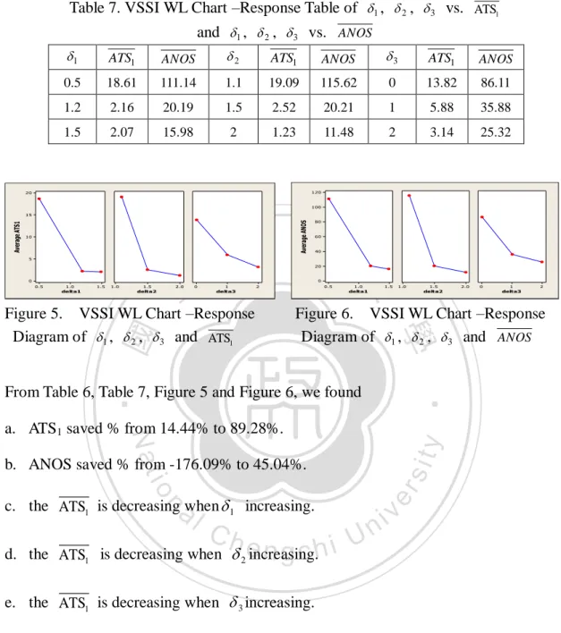
(43) 5 and Figure 6). Table 7. VSSI WL Chart –Response Table of 1 , 2 , 3 vs.. ATS1. and 1 , 2 , 3 vs. ANOS 1. ATS1. ANOS. 2. ATS1. ANOS. 3. ATS1. ANOS. 0.5. 18.61. 111.14. 1.1. 19.09. 115.62. 0. 13.82. 86.11. 1.2. 2.16. 20.19. 1.5. 2.52. 20.21. 1. 5.88. 35.88. 1.5. 2.07. 15.98. 2. 1.23. 11.48. 2. 3.14. 25.32. 120. 20. 100. Average ANOS. Average ATS1. 15. 10. 5. 80. 政 治 大 60. 40. 20. 0 0.5. 1.0. 立 VSSI WL Chart –Response. delta1. 1.5. 1.0. 1.5. 2.0. 0. delta2. 1. 0. 0.5. 2. ‧ 國. 1.5. 1.0. ATS1. 0. 1. y. sit. io. n. c. the ATS1 is decreasing when 1 increasing.. engchi. d. the ATS1 is decreasing when 2 increasing.. er. b. ANOS saved % from -176.09% to 45.04%.. i n U. v. e. the ATS1 is decreasing when 3 increasing. f.. the ANOS is decreasing when 1 increasing.. g. the ANOS is decreasing when 2 increasing. h.. 2. delta3. ‧. Nat. a. ATS1 saved % from 14.44% to 89.28%.. Ch. 2.0. Figure 6. VSSI WL Chart –Response Diagram of 1 , 2 , 3 and ANOS. From Table 6, Table 7, Figure 5 and Figure 6, we found. al. 1.5. delta2. 學. Figure 5. Diagram of 1 , 2 , 3 and. 1.0. delta1. delta3. the ANOS is decreasing when 3 increasing.. (4) ATS1 Analysis of VP WL Chart and ATS1 Comparison between FP WL Chart and Specified VP WL Chart 23.
(44) Under 0 0 , 02 1 , n0 5 , h0 1 , 0 0.0027 (or ARL0 = 370.37), p * 0.5 and a 0.6 . Consider the levels of the parameters, 1 = (0.5, 1.2, 1.5),. 2 = (1.1, 1.5, 2), 3 = (0, 1, 2), h2 = (0.1, 0.5, 0.9), (n1, n2): (2, 6), (3, 10), (4, 20) and 1 = (0.00135, 0.002025, 0.0027). The 27 combinations are arranged by L27(313). The ATS1s of the 27combinations of the VP chart are listed in Table 8.. 立. 政 治 大. ‧. ‧ 國. 學. n. er. io. sit. y. Nat. al. Ch. engchi. 24. i n U. v.
(45) ATS1 and ANOS for VP WL Chart and ATS1 saved % and ANOS Saved % Compared to FP WL Chart. Table 8.. Specified VP (n1, n2, h2, 1 ). FP. ATS1. ANOS. 2. 3. (n1, n2). h2. h1. 1. 2. ATS1. ANOS. ARL1. ANOS. saved %. saved %. 1. 0.5. 1.1. 0. (2,6). 0.1. 3.70. 0.0027. 0.0027. 93.73. 551.38. 109.54. 547.70. 14.44%. -0.67%. 2. 0.5. 1.1. 1. (3,10). 0.5. 1.20. 0.0020. 0.0044. 18.02. 138.14. 38.67. 193.35. 53.39%. 28.55%. 3. 0.5. 1.1. 2. (4,20). 0.9. 1.01. 0.0014. 0.0230. 8.49. 64.41. 29.36. 146.81. 71.08%. 56.12%. 4. 0.5. 1.5. 0. (2,6). 0.5. 2.50. 0.0027. 0.0027. 5.00. 38.35. 7.79. 38.93. 35.84%. 1.48%. 5. 0.5. 1.5. 1. (3,10). 0.9. 1.04. 0.0020. 0.0044. 3.14. 26.26. 5.90. 29.51. 46.74%. 11.01%. 6. 0.5. 1.5. 2. (4,20). 0.1. 1.06. 0.0014. 0.0230. 2.13. 28.22. 6.20. 31.02. 65.64%. 9.03%. 7. 0.5. 2. 0. (2,6). 0.9. 1.30. 0.0027. 0.0027. 1.94. 12.06. 2.36. 11.80. 18.00%. -2.19%. 8. 0.5. 2. 1. (3,10). 0.1. 1.36. 0.0020. 0.0044. 0.55. 13.27. 2.31. 11.55. 76.30%. -14.88%. 9. 0.5. 2. 2. (4,20). 0.5. 1.03. 10. 1.2. 1.1. 0. (4,20). 0.1. 11. 1.2. 1.1. 1. (2,6). 12. 1.2. 1.1. 2. (3,10). 13. 1.2. 1.5. 0. (4,20). 14. 1.2. 1.5. 1. (2,6). 15. 1.2. 1.5. 2. (3,10). 16. 1.2. 2. 0. (4,20). 17. 1.2. 2. 1. (2,6). 0.1. 18. 1.2. 2. 2. (3,10). 0.5. 19. 1.5. 1.1. 0. (3,10). 0.1. 20. 1.5. 1.1. 1. (4,20). 0.5. 21. 1.5. 1.1. 2. (2,6). 0.9. 22. 1.5. 1.5. 0. (3,10). 23. 1.5. 1.5. 1. 24. 1.5. 1.5. 25. 1.5. 26 27. 13.32. 47.46%. -45.26%. 21.67. 108.35. 80.46%. 58.05%. 5.10. 25.51. 61.31%. 15.65%. 0.9. 1.04. 0.0027. 0.0027. 1.39. 14.94. 3.60. 17.99. 61.50%. 16.92%. 0.5. 1.03. 0.0020. 0.0128. 1.39. 21.85. 4.14. 20.72. 66.53%. -5.45%. 0.9. 1.30. 0.0014. 0.0032. 1.81. 11.71. 2.42. 12.09. 25.06%. 3.18%. 0.1. 1.36. 0.0027. 0.0027. 0.25. 12.63. 2.21. 11.05. 88.60%. -14.23%. 0.9. 1.01. 0.0020. 0.0128. 1.19. 18.22. 1.88. 9.41. 37.05%. -93.60%. 3.70. 0.0014. 0.0032. 0.30. 8.34. 1.59. 7.96. 80.94%. -4.75%. 1.20. 0.0027. 0.0027. 0.68. 11.10. 1.63. 8.12. 57.93%. -36.68%. 0.0014 0.0061 0.93 24.67 a v 1.03 l 0.0027 0.0027 0.53 20.06i n C h 0.0029 1.46 U9.69 1.30 0.0020 engchi. 9.86. 49.32. 90.53%. 49.97%. 2.70. 13.51. 80.37%. -48.44%. 2.04. 10.19. 28.44%. 4.86%. 0.5. 1.20. 0.0014. 0.0061. 0.88. 13.58. 3.01. 15.07. 70.87%. 9.85%. (4,20). 0.9. 1.01. 0.0027. 0.0027. 0.94. 19.72. 1.79. 8.97. 47.43%. -119.90%. 2. (2,6). 0.1. 3.70. 0.0020. 0.0029. 0.20. 8.43. 1.64. 8.18. 87.66%. -3.06%. 2. 0. (3,10). 0.9. 1.04. 0.0014. 0.0061. 1.06. 10.78. 1.67. 8.34. 36.74%. -29.14%. 1.5. 2. 1. (4,20). 0.1. 1.06. 0.0027. 0.0027. 0.19. 19.23. 1.39. 6.97. 86.05%. -176.09%. 1.5. 2. 2. (2,6). 0.5. 2.50. 0.0020. 0.0029. 0.70. 7.51. 1.39. 6.95. 49.70%. -7.95%. 0.0014. n. 1.36. FP-ARL VP-ATS 1. sit. io. er. Nat. Note: ATS1 saved %:. 學. ‧ 國. 2.66. 0.5. 0.0230 治 1.40 19.35 政 1.06 0.0020 0.0128 4.24 大 45.46 立0.0014 0.0032 1.97 21.52 2.50. y. 1. ‧. No.. 1. FP-ARL1 % , ANOS saved %:. FP-ANOS VP-ANOS . FP-ANOS %. To investigate the effect of 1 , 2 and 3 on the ATS1 and ANOS, the response table and response diagram show the results of the sensitivity analysis (Table 9, Figure 7 and Figure 8). 25.
(46) VP WL Chart –Response Table of 1 , 2 , 3 vs.. Table 9.. ATS1. and 1 , 2 , 3 vs. ANOS 1. ATS1. ANOS. 2. ATS1. ANOS. 3. ATS1. ANOS. 0.5. 14.93. 99.05. 1.1. 14.53. 98.92. 0. 12.26. 81.82. 1.2. 1.47. 18.42. 1.5. 1.75. 20.08. 1. 3.05. 30.92. 1.5. 0.77. 14.85. 2. 0.89. 13.32. 2. 1.86. 19.59. 16. 100. 14. 90 80. Average ANOS. Average ATS1. 12 10 8 6 4. 70 60 50 40 30. 2. 20 10. 0 0.5. 1.2. delta1. 1.5. 1.1. 1.5. 2.0. 0. delta2. 1. delta3. 0.5. 2. 1.2. 1.5. 1.1. 0. 1. 2. delta3. 8. FP WL chart –Response 政 治Figure 大of , , and Diagram 1. 2. ‧ 國. 學. From Table 8, Table 9, Figure 7 and Figure 8, we found. ‧. a. ATS1 saved % from 14.44% to 90.53%.. sit. y. Nat. b. ANOS saved % from -176.09% to 58.05%.. n. d. the ATS1 is decreasing when 2 increasing.. Ch. engchi. e. the ATS1 is decreasing when 3 increasing.. f. the ANOS is decreasing when 1 increasing. g. the ANOS is decreasing when 2 increasing. h. the ANOS is decreasing when 3 increasing.. 26. er. io. c. the ATS1 is decreasing when 1 increasing.. al. 2.0. delta2. Figure 7. VP WL Chart –Response Diagram of 1 , 2 , 3 and ATS1. 立. 1.5. delta1. i n U. v. 3. ANOS.
數據
+7
相關文件
In this paper, we have shown that how to construct complementarity functions for the circular cone complementarity problem, and have proposed four classes of merit func- tions for
In our AI term project, all chosen machine learning tools will be use to diagnose cancer Wisconsin dataset.. To be consistent with the literature [1, 2] we removed the 16
n Media Gateway Control Protocol Architecture and Requirements.
To decide the correspondence between different sets of fea- ture points and to consider the binary relationships of point pairs at the same time, we construct a graph for each set
In order to detect each individual target in the crowded scenes and analyze the crowd moving trajectories, we propose two methods to detect and track the individual target in
In this study the GPS and WiFi are used to construct Space Guidance System for visitors to easily navigate to target.. This study will use 3D technology to
This study conducted DBR to the production scheduling system, and utilized eM-Plant to simulate the scheduling process.. While comparing the original scheduling process
The Earned Value Management (EVM) is an international standard for project cost control, which provides a promising tool for project cost control practice of the middle
